en fr

HAL Id: hal-03058548

https://hal.archives-ouvertes.fr/hal-03058548

Submitted on 11 Dec 2020

HAL is a multi-disciplinary open access

archive for the deposit and dissemination of

sci-entific research documents, whether they are

pub-lished or not. The documents may come from

teaching and research institutions in France or

abroad, or from public or private research centers.

L’archive ouverte pluridisciplinaire HAL, est

destinée au dépôt et à la diffusion de documents

scientifiques de niveau recherche, publiés ou non,

émanant des établissements d’enseignement et de

recherche français ou étrangers, des laboratoires

publics ou privés.

feldspars

Eric Bringuier

To cite this version:

Eric Bringuier. Disorder-enhanced luminescence kinetics in volcanic feldspars. EPJ Web of

Confer-ences, EDP SciConfer-ences, 2020, 244, �10.1051/epjconf/202024401012�. �hal-03058548�

Disorder-enhanced luminescence kinetics

in volcanic feldspars

Eric Bringuier1

eric.bringuier@univ-paris-diderot.fr

1_{Matériaux et Phénomènes Quantiques, Unité mixte 7162 CNRS & Université de Paris, 5 rue Thomas Mann, 75013} Paris, France

Abstract. A granitic feldspar is well-ordered and has a stable thermoluminescence signal enabling its

dating with high reliability. In contrast, a volcanic feldspar (sanidine) exhibits a slight cristallographic disorder and an anomalously fast fading of the thermoluminescence signal (Visocekas et al. 2014). It is shown here how disorder changes the decay of the signal and enhances the kinetics, while the increase in the microscopic complexity plays no role.

1. Introductory description of the

phenomenon and the material

We begin with a few definitions [1] of the terms used in this paper.

Definition of thermoluminescence (TL). It is the

luminescence I emitted upon heating a mineral at a constant rate dT/dt where T (t) is the temperature (time). If the I-vs-T curve at a given rate is reproducible, it allows for dating of the mineral.

The luminescent material. It is a K-feldspar

(K-aluminosilicate) which can be found in two varieties, called sanidine and microcline. The latter variety is also called granitic whereas the former is a volcanic feldspar. Quotation from [1]: « Sanidines and microclines have the same composition and similar lattice structures. They are two extreme phases of KAlSi₃O₈ feldspars. Sanidine is the high-temperature form whereas microcline is stable at low temperatures, or below approximately 450 °C. [...] The angular difference between their optical axes is very small; an angle of 90° in sanidine becomes 87° 40' in ‘maximum’ microcline. Microcline is ordered, whereas sanidine is still a crystal but ‘disordered’. The 25 % Al atoms substituted for Si are randomly distributed in sanidine, whereas they are ordered in microcline. » The quick cooling of a volcanic feldspar quenches its high-temperature lattice structure which is metastable at room temperature [2].

Microscopic origin of the luminescence. It is due to

a very small fraction of impurities (called activators) interspersed in the solid lattice. In feldspars, the presence of Fe3+ results in light-emitting centres in the blue and far-red ranges. Besides light-emitting centres, the mineral hosts electron traps whose energy levels lie in the 7.7-eV forbidden band gap. Once detrapped, an electron can be captured near the centre and excite it. A subsequent radiative deexcitation of the centre gives rise to a luminescence whose sensitivity to temperature is due to the fact that electron detrapping is thermally activated. As the temperature is raised the freed electrons continually feed the light-emitting centres.

The thermoluminescence phenomenon. When a

microcline sample is stored at room temperature, its TL

signal does not fade during storage. In contrast, the TL signal of sanidine is observed to fade at a rate −25 % per year. Such a fast fading is called anomalous. Because its

I-vs-T curve is not reproducible over time, sanidine

cannot be used for dating by TL.

The goal of this paper is to understand the physics of the so-called anomalous fading of sanidine. What is it that links the ill-ordered nature of sanidine to its inability to retain the energy released (in part) as the TL signal emitted upon heating? To answer this question, we shall examine what happens at a constant temperature because isothermal physics is easier to deal with. In section 2 we recall the state of knowledge of the isothermal luminescence decay in microcline and more generally speaking well-ordered minerals. In section 3 we examine how the tunnelling model which accounts for the kinetics in a well-ordered material can be rescued if the material exhibits some disorder. In section 4 we parallel electron transfer by tunnelling and energy transfer by exchange; the latter mechanism has been investigated in more detail. In section 5 we show how our electron-transfer problem can be traded for an energy-transfer problem for which a mathematical solution has already been reached. Section 6 explains why the complexity of disorder is not involved.

2. Isothermal luminescence decay in

well-ordered materials

The time-resolved luminescence intensity I(t) in feldspars at a constant temperature does not follow the usual exponential decay law of phospho- or fluorescence. Decay is much slower, typically I(t)  1/t at large times. This had previously been observed in Mn-activated calcium carbonate (CaCO₃, 6-eV band gap): figure 2 of [3] shows constant It vs t over almost three decades of time. As I was independent of T in the range 80–180 K, a tunnel-based decay mechanism had been suggested [3]. In Mn-activated zinc silicate (Zn₂SiO₄, 5-eV band gap) a similar very slow and athermal decay was observed later by Avouris and Morgan [4]. Quotation: « Both phosphorescence and photostimulated luminescence intensities are found to decay as the

reciprocal of the time, a result which requires a different interpretation from that given by the usual model of electron release from a distribution of trap levels. To account for these results we propose a new model based on the radiative recombination of electrons and holes through tunnelling from shallow traps or from excited states of the deeper traps. A simple expression is derived which describes the decay of both types of luminescence in phosphors under very general conditions for which tunnelling is the dominant recombination mechanism. »

In a word, luminescence in Mn-activated calcium carbonate and zinc silicate is due to variable-range

tunnelling. By tunnelling a trapped electron escapes to a

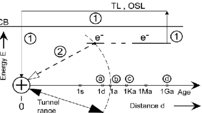
capture centre where it will excite the light-emitting impurity (activator). It is alternatively said that the tunnelled electron ‘recombines’ at the centre. As time goes by, trapped electrons have been captured by nearby capture/recombination centres, and subsequently electrons can be captured only by remoter centres. A longer distance entails a slower decay rate. This has been called the gruyère [5] or Swiss cheese [6] model: the diameter of a spherical volume freed from trapped electrons increases logarithmically with time; see fig. 1.

Fig. 1. The gruyère or Swiss cheese model of

tunnelling-induced luminescence in a solid. From [6].

A more general decay law was obtained later by Huntley [7]. Quotation: « Luminescence decay with time often shows a power-law dependence of the form intensity I  t−m, where t is time and m is usually in the range 1–1.5. [...] This power law can result from the tunnelling of trapped electrons to recombination centres that are randomly distributed, and [...] the range of exponents matches that of the observations. The explanation accounts for the most extreme case of an observed t−1.06 dependence extending over nine decades of time. »

Let us reckon luminescence I(t) = N₀|d/dt| in photon per second, where N₀ is the initial number of trapped electrons able to excite a light-emitting centre, and (t)=

N(t)/N₀ is the fraction of as yet untransferred electrons at time t. (This formula for I(t) omits the radiative yield which effectively reduces N₀.) Let n_A denote the number density of recombination centres capturing electrons released from traps, and let 1/(r) = s₀exp(−r) denote the rate of electron tunnelling from a trap to a recombination centre, as a function of their separation distance r. The number of electron-capture centres in a sphere of radius −1 is n ~ A = 4−3 3 nA.

For a time t >> s₀−1, Huntley arrives at (t)  exp

[

]

The unsigned argument of the exponential function is the number of capture centres in a sphere of radius −1ln(s₀t)

which grows logarithmically with time. This is in keeping with the gruyère or Swiss cheese model of fig. 1. For plausible values of n~_A and over a wide time range,

I(t) is found to be closely approximated by a power law A/tm where 0.95 m1.5.

3. The tunnelling model in sanidine

3.1. The problem

From the above expression of n~_A, it is seen that I(t)  |d/dt| cannot depend on temperature. This comes about because tunnelling is an athermal mechanism. Now in sanidine the fading of the TL signal is observed to depend on the storage temperature of the sample. The crucial point is that no loss of TL is observed if the sample is stored at liquid-nitrogen temperature [6].

A possible explanation for a temperature dependence was proposed long ago [3, 4]: electrons are not only tunnelled out of the ground state of a trap lying at level

E_g but also out of an excited state lying at level E_e > E_g. Since the excited state is populated thermally according to a Boltzmann factor exp(−(E_e− E_g)/kT), this would account for the freezing of electron release at lower temperatures. This scenario predicts an Arrhenius dependence not observed in sanidine. The softer actual dependence might be accounted for by assuming a continuum of excited states. This mathematical assumption is, however, not physically realistic. The next subsection offers an alternative explanation. 3.2. The physics of a disordered solid

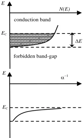
Room-temperature fading is observed only in the ill-ordered feldspars known as sanidines. When a crystal exhibits some disorder, whether translational or orientational, its energy-band structure is altered. Between the first unoccupied band of extended (Bloch) states and the band-gap where no electron state is allowed, there is an energy range of localized (Mott) states, called the band tail. A state in the band tail is quantum-mechanically allowed but localized. This is shown in figure 2 after [8].

E

N(E)

E

E

forbidden band-gap

conduction band



E

E

Fig. 2. The allowed one-electron quantum states in a

disordered solid. Besides the extended states of the conduction band lying above the mobility edge E_c, there exists a tail of localized states (hatched area) over a range E. The conduction band is virtually empty if the solid is semiconducting. Top: density of allowed states N(E). Bottom: decay length −1 of the localized states; at the mobility edge, −1 is becoming infinite which corresponds to an extended (Bloch) state. After figure 6.8 of [8].

Let us give details about the physical nature of the electron states involved. A Bloch state of pseudo-momentum p = h_k and energy E(p) is a travelling matter

wave with a group velocity E/p expressing the mean

flow of the probability of presence. Were the lattice perfectly periodic, that wave would be a stationary solution of Schrödinger's wave equation, i.e. with an infinite lifetime. Imperfections of the lattice, whether static (flaws and impurities) or dynamic (thermal vibrations), entail a finite lifetime and a finite velocity-relaxation time _v(p) of the Bloch state. As a result the mean free path of an electron in the Bloch state,  =

v_g_v, is finite. Then,

(i) under no electric force, an initially sharply peaked electron ensemble spreads out isotropically with a Fick diffusion coefficient D = 2/3_v; (ii) under a force F = e_(−V) derived from the macroscopic electric potential V, where e_ is the signed electron charge, electrons drift along the force at an ensemble-average velocity _vF/m* where the effective mass m* is determined from the dispersion relation E(p).

In contrast, a state in the band tail is an evanescent

matter wave which does not propagate; a

pseudo-wavevector k is not relevant. The spatial extension of the evanescent matter wave, −1, is finite. If such a state is occupied by an electron and there is an empty state nearby, then the electron can ‘hop’ from the occupied to the empty state if the overlap of the two wave functions is not too small. The mechanism is tunnelling, but since there is a misfit in the energies of the initial and final states, the lattice has to supply or collect the energy difference in the guise of a phonon. Thereby an electron can walk at random between band-tail states lying at almost the same energy. In some steps energy is supplied by the lattice while in others it is released to the lattice.

In the simplest (‘nearest-neighbour’) scenario, a step has a length −1 and the hopping frequency  depends on the tunnelling probability per unit time and the rate at which the lattice can supply energy. Statistically speaking, the random walk is characterised by a Fick diffusivity D. Taking hopping to be isotropic, D is given by −2/3.

A note on nomenclature is important. The usual parlance of disordered conductors makes use of the word ‘mobility’ in e.g. the phrase ‘mobility edge’ denoting the energy border E_c between extended (Bloch) and localized (Mott) states. However, the quantitative definition of mobility  refers to the response of an electron to an applied force, with  = _v/m* _{in the Drude}

model [9]. In our problem, there is no force and electrons move by diffusion. It is more appropriate to speak of a ‘diffusivity edge’ as advocated by Butcher [10] when discussing mobility * _{and diffusivity D}* _{as functions of}

the electron energy E. Quotation: « we would then speak of ‘energy-dependent diffusivity’ instead of ‘ energy-dependent mobility’ and ‘diffusivity edge’ instead of ‘mobility edge’. It is important to emphasize that what is involved here is more than a matter of semantics. The terminology which is growing up in work on amorphous materials may ultimately lead to physical confusion because *_{(E) is much more intimately related to}

diffusivity than mobility. [...] The diffusive nature of the electronic motion in amorphous materials suggests that a greater emphasis will be placed on diffusivity than has been appropriate in crystalline materials. The energy-dependent diffusivity provides the obvious tool for this purpose. By inserting a factor of 1/kT so that the result has the dimensions of mobility, we gain nothing in the formalism and lose something in the conceptual simplicity of the subject. » (See also [11].)

Two hopping mechanisms are met in practice: (i) nearest-neighbour hopping giving an Arrhenius dependence D(T)  exp(−E₀/kT);

(ii) optimum-range hopping involving second, third... neighbours, such that

D(T)  exp

(

)

3.3. Adapting the tunnelling model to the case of sanidine

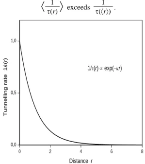
Call D (donor) an occupied electron trap lying in the band tail. The distance r between the trapped electron and a recombination centre acting as an electron acceptor A, is no longer constant in time. Because the electron can hop from a band-tail state to another, the distance r becomes a function of time for a given electron. The distance is a random variable in that, in a statistical ensemble of electrons in Gibbs’ sense, different electrons will have different histories. Denote Gibbs-ensemble averaging by ... Insofar as disorder is homogeneous, .. may be replaced by spatial averaging. The spatial average over a large volume is identical with the average over a large number of realisations, that is to say a Gibbs-ensemble average. This is an ergodicity property in space instead of time [12]. Now the tunnelling rate 1/(r)  exp(−r) shown in figure 3 is a convex function of distance r so that, over a range of values of r,





Fig. 3. The tunnelling rate per unit time 1/ as a function of

distance r (arbitrary units).

Tunnelling is enhanced by the fact that r is a random variable owing to the diffusive motion of band-tail electrons. Enhancement can be strong because of the strong dependence of 1/ on r. This qualitatively explains why the phenomenon of hopping between band-tail states is able to enhance the kinetics. We shall now address the phenomenon quantitatively. To this end we first recall the knowledge gained from exchange-mediated energy-transfer studies in luminescent solids.

4. Energy transfer by exchange

4.1. What is meant by energy transfer?

We quote the Encyclopedia of Spectroscopy and

Spectrometry [13]: « Energy transfer refers to a process

in which an excited atom or molecule (donor) transfers its excitation energy to an acceptor atom or molecule

during the lifetime of the donor excited state. [...] As a result of energy transfer, the donor returns to its ground state while the acceptor is promoted to its excited state. If the acceptor is a luminescent species, it can emit by virtue of energy transfer, that is, the acceptor luminesces as a result of the excitation of the donor. Such a luminescence is called ‘sensitized luminescence’, and some textbooks use the terms ‘sensitizer’ and ‘activator’ instead of ‘donor’ and ‘acceptor’. » This is pictured in figure 4. energy

D

D

A

A

Fig. 4. Energy transfer from donor D to acceptor A. In the case

of an energy difference between the excited state of D and that of A, the transfer has to be assisted by a phonon. After [13].

Donor (D) to acceptor (A) energy transfer can proceed via two coupling mechanisms, termed multipolar and exchange. This terminology originates in the definitions of Coulomb and exchange integrals. Let

(r₁, r₂)  _D(r₁)_A(r₂) − _D(r₂)_A(r₁). denote the two-electron D-A wave-function for parallel spins. It is antisymmetric in the exchange of electrons 1 and 2. The coupling involves the matrix element

(

|

2

4|r₁−r₂|

|

)

Coulomb integral C_DA − exchange integral J_DA. Depending on the symmetries of the wave functions, the Coulomb integral is dipolar, quadrupolar etc, which is why one speaks of multipolar coupling. The basic studies are Förster’s [14] (Dexter’s [15]) for multipolar (exchange) coupling.

In the remainder of the paper we shall be interested in exchange-mediated D-to-A energy transfer. It is epitomized by Rice [16] in the following sentences: « The exchange integral effectively reflects the initial overlap of the wave functions of donor and acceptor molecules, [...] weighted by the Coulomb energy,

e2/4|r₁− r₂|, of interaction between these initial and final states. Provided that both initial- and final-state wave functions are appreciable in the same region of space, the exchange integral is not negligible. Since the eigenfunctions decay as exp(−r/a) with a an approximate Bohr radius for these eigenfunctions ( 0.14 nm), the transfer probability [roughly] varies as the square of the exchange integral, i.e.

l(r) = A exp(−2r/a).

[...] The pre-exponential factor of the transfer probability is

A 



where f_D() is the frequency-dependent donor emission spectrum (phosphorescence) and _A() the absorption spectrum of the acceptor when the electron spin restriction is removed. »

4.2. Electron transfer by tunnelling vs energy transfer by exchange

We again quote Rice’s review [16]: « The dependence on the distance of separation of donor and acceptor is similar for energy transfer by the exchange effect and electron transfer by tunnelling. The probability of energy transfer from donor to acceptor (electron scavenger) is

l(r) = exp[−(r − R)]

where   1014 s−1 and −1  0.1 nm. In the same manner as energy transfers non-radiatively, the electron transfers rapidly (less than 0.01 ps or so) during which time the donor and acceptor nuclei remain essentially frozen (Franck-Condon principle). Henglein has emphasised the similarity of energy and electron transfer processes by representing electron transfer as the overlap of the donor oxidation spectrum and the acceptor reduction spectrum weighted by the orbital overlap of the donor anion and acceptor states. It is this latter term which leads to the exponential dependence of l(r). »

In the next subsection we avail ourselves of this formal similarity to swap the electron-transfer problem for an energy-transfer problem which has already been investigated quantitatively.

5. The solution

5.1. The two-body problem in Smoluchowski's stochastic mechanics

In the physical problem at stake in this paper, we have to do with electron donors D which move randomly by hopping, and electron acceptors A fixed at definite positions. Let us contemplate the reverse mathematical problem where a donor D is fixed while acceptors A move by diffusion. The number density n_A of acceptors is governed by Fick's second law,

n_A

t + div(−DAnA) = 0,

involving the diffusivity D_A of A. This results in a continuous-time random walk of A,

x_A(t) = x_A(0) and x_A(t)2_{ − x} A(t)

2 _{= 2D} At

in one dimension [17]. On the average, A does not move. It spreads about its initial position x_A(0).

We now consider the more general, two-body problem where both A and D are diffusing. In addition we have

x_D(t) = x_D(0) and x_D(t)2 − x_D(t)2 = 2D_Dt,

and the covariance x_D(t)x_A(t) − x_D(t)x_A(t) vanishes if the random variables x_A and x_D are independent. The upshot is that the D-A distance keeps constant on the average,

x_D(t) − x_A(t) = x_D(0) − x_A(0), while its variance grows up linearly in time,

(x_D(t)−x_A(t))2 − x

D(t)−xA(t)2 = 2DDt + 2DAt.

The relative motion is therefore a stochastic process characterized by a coefficient of mutual diffusion,

D = D_D + D_A.

This enables us to trade the problem of fixed donors and moving acceptors for the problem of moving donors and fixed acceptors. As a result, if the problem of exchange-mediated energy transfer from static D to moving A is solved, then the problem of tunnelling electron transfer from moving D to static A is solvable. It turns out that the former problem has indeed been solved, and this is the subject of the next subsection.

5.2 The solution of energy transfer by exchange Just as in section 2, let (t)=N(t)/N₀ denote the fraction of untransferred electrons at time t. The luminescence (in photon/s) is N₀|d/dt|. As trapped electrons can hop, (t) will be less than ₀(t) as calculated by Huntley in his model of static electron donors [7]. We write

(t) = ₀(t)_D(t),

where ₀(t) is the limiting form of (t) when diffusion is frozen i.e. as D → 0. The calculation of _D due to electron hopping is possible using the study of exchange-mediated energy transfer by Allinger and Blumen [18]. They found that

₀(t) = exp

[

]

where g₃(u)  ln3u + g₃₂ln2u for u >> 1 and g₃₂  1.73165. The g₃₂ term is a small correction to Huntley's result given in section 2. Besides,

_D(t) = exp

[

]

The luminescence intensity is proportional to

|

|

[

]

[

]

In the case that ln(s₀t) >> 1 this may be simplified to

|

|

[

]

For vanishing D i.e. _D = 1, Huntley has shown that |d/dt|  A/tm over a wide range of times t >> s₀−1. We now address the correction due to non-vanishing D for t = 3x107 s  1 year. Again we have to resort to typical, plausible values of the microscopic parameters. With −1  0.1 nm and n_A = 5x1017 cm−3 i.e. n~_A = 3x10−6 [7], we compute s₀t  1021 and ₀(t) = exp(−0.36) so that traps have been slightly depleted. For a hopping diffusivity D = 10−6 m2/s, (2Dt)1/2  5x1010. The ensuing reduction in the number of excited donors is _D(t) = exp[−3n~_A (2Dt)1/2ln2(s₀t)], whence _D(t)  exp(−109) means that luminescence has been drastically exhausted by hopping. What is the justification for choosing D = 10−6 m2/s? In a disordered poor conductor, D = kT and e does not exceed 1 cm2/V.s at room T (this is related to the so-called Ioffe-Regel criterion) [8]. Thus we have taken an

excess value of D and, in practice, TL fading over one year will be less drastic but it can be very significant.

6. Synopsis

This paper has been concerned with the way a luminescence decay can be affected by the appearance of a cristallographic disorder. The disorder gives rise to localized electron states in a band tail lying below the conduction band of extended (Bloch) states of the solid. An electron in the band tail can hop between states with a small, temperature-dependent diffusivity. Hopping enhances an electron’s probability per unit time to tunnel toward a recombination centre and activate a light-emitting centre lying nearby. The enhancement of tunnelling depends on temperature, and it is prevented at liquid-nitrogen temperature where diffusivity is lower.

Generally speaking, disorder generates complexity in the sense that a large number of microscopic configurations become possible. If the ‘disorder variable’ is a random scalar field endowed with statistical homogeneity, disorder is characterised by a (position-independent) average and 2-point, 3-point... spatial correlation functions [12]. Complexity may then be assessed by the number of correlation functions that are needed to describe the phenomenon. In contrast, simplicity may be associated with the need of resorting to the average and/or the 2-point function only. For example, in the scattering of light by the density fluctuations of an almost homogeneous medium, no role is played by the 3-point, 4-point... correlation functions of the random refraction-index field [19]. In the issue at hand in this paper, the disorder shows up through one single parameter, namely the diffusivity of band-tail electrons which reflects a 2-time velocity-correlation function [20]. In this sense complexity plays no role. It is a pleasure to acknowledge Raphaël Visocekas (Université Denis Diderot) for a number of stimulating and clarifying conversations about thermoluminescence. The present investigation on anomalous luminescence decays owes much to interactions with the late André Geoffroy (Université Pierre et Marie Curie) and Jacques Duran (CNRS).

References

1. R. Visocekas, C. Barthou, P. Blanc, Radiation

Measurements 61 52–73 (2014)

2. N. W. Ashcroft, N. D. Mermin, Solid State Physics (Holt, Rinehart & Winston, New York, 1976) pp. 620–1 3. R. Visocekas, T. Ceva, C. Marti, F. Lefaucheux, M. C. Robert, phys. stat. sol. (a) 35 315–327 (1976)

4. P. Avouris, T. N. Morgan, J. Chem. Phys. 74 4347– 4355 (1981)

5. R. Visocekas, PACT 3 258–265 (1979)

6. G. Guérin, R. Visocekas, Radiation Measurements 79 1–6 (2015)

7. D. Huntley, J. Phys. Condens. Matter 18 1359–1365 (2006)

8. N. F. Mott, E. A. Davis, Electronic Processes in

Non-Crystalline Materials 2nd edn (Clarendon, Oxford,

1979)

9. E. Bringuier, Eur. J. Phys. 39 025101 (2018) 10. P. N. Butcher, J. Phys. C 5 3164–3167 (1972) 11. E. Bringuier, Phil. Mag. B 77 959–964 (1998) 12. J. M. Ziman, Models of Disorder: The theoretical

physics of homogeneously disordered systems

(Cambridge University Press, Cambridge, 1979) chap. 3 13. M. A. Omary, H. H Patterson, Luminescence theory, in: Encyclopedia of Spectroscopy and Spectrometry 2nd edn, edited by J. C. Lindon, G. E. Tranter, D. W. Koppenaal (Elsevier, Amsterdam,1999) pp. 1186–1207 14. T. Förster, Z. Naturforsch. A 4 321–327 (1949) 15. D. L. Dexter, J. Chem. Phys. 2 836–850 (1953) 16. S. A. Rice, Long-range transfer effects and

diffusion-controlled reactions, in: Comprehensive Chemical

Kinetics vol. 25 (Elsevier, Amsterdam, 1985) pp. 71– 104

17. S. Chandrasekhar, Rev. Mod. Phys. 15 1–89 (1943);

Rev. Mod. Phys. 21 383–388 (1949)

18. K. Allinger, A. Blumen, J. Chem. Phys. 75 2762– 2771 (1981)

19. P. Debye, A. M. Bueche, J. Appl. Phys. 20 518 (1949)

20. G. H. Wannier, Statistical Physics (Wiley, New York, 1966) chap. 23