HAL Id: hal-01672001
https://hal.inria.fr/hal-01672001
Preprint submitted on 22 Dec 2017
HAL is a multi-disciplinary open access
archive for the deposit and dissemination of
sci-entific research documents, whether they are
pub-lished or not. The documents may come from
teaching and research institutions in France or
abroad, or from public or private research centers.
L’archive ouverte pluridisciplinaire HAL, est
destinée au dépôt et à la diffusion de documents
scientifiques de niveau recherche, publiés ou non,
émanant des établissements d’enseignement et de
recherche français ou étrangers, des laboratoires
publics ou privés.
Metric approximation of minimum time control systems
Jean-Baptiste Caillau, Jean-Baptiste Pomet, Jeremy Rouot
To cite this version:
Jean-Baptiste Caillau, Jean-Baptiste Pomet, Jeremy Rouot. Metric approximation of minimum time
control systems . 2017. �hal-01672001�
control systems
∗
J.-B. Caillau
†J.-B. Pomet
‡J. Rouot
§November 2017
Abstract
Slow-fast affine control systems with one fast angle are considered. An approximation based on standard averaging of the extremal is defined. When the drift of the original system is small enough, this approximation is metric, and minimum time trajectories of the original system converge towards geodesics of a Finsler metric. The asymmetry of the metric ac-counts for the presence of the drift on the slow part of the original dyna-mics. The example of the J2effect in the two-body case in space mechanics
is examined. A critical ratio between the J2 drift and the thrust level of
the engine is defined in terms of the averaged metric. The qualitative behaviour of the minimum time for the real system is analyzed thanks to this ratio.
Keywords. Slow-fast control systems, minimum time, averaging, Finsler metric, J2 potential of two-body problem
MSC classification. 49K15, 70Q05
1
Averaging of slow-fast minimum time control
systems
We consider the following slow-fast control system on an n-dimensional manifold M : 9 I “ εF0pI, ϕ, εq ` ε m ÿ i“1 uiFipI, ϕ, εq, |u| “ b u2 1` ¨ ¨ ¨ ` u2mď 1, (1) 9 ϕ “ ωpIq ` εG0pI, ϕ, εq ` ε m ÿ i“1 uiGipI, ϕ, εq, ωpIq ą 0, (2)
∗Work supported by the French Space Agency (CNES R&T contract no.
R-S13/BS-005-012).
†LJAD, Univ. Cˆote d’Azur & CNRS/Inria, Parc Valrose, F-06108 Nice
([email protected]). Also supported by FMJH and EDF (PGMO grant no. 2016-1753H).
‡Inria Sophia Antipolis M´editerran´ee, Univ. Cˆote d’Azur, 2004 route des lucioles, F-06902
Valbonne ([email protected]).
§Ecole´ Polytechnique F´eminine, 2 rue Sastre, F-10430 Rosi`eres-pr`es-Troyes
Metric approximation of minimum time control systems 2
with I P M , ϕ P S1, u P Rm, and fixed extremities I
0, If, and free phases ϕ0, ϕf. All the data is periodic with respect to the single fast angle ϕ, and ω is assumed to be positive on M . Extensions are possible to the case of several phases but resonances have then to be taken into account. According to Pontrjagin maximum principle, time minimizing curves are projections onto the base space M ˆ§1 of integral curves (extremals) of the maximized Hamiltonian below:
HpI, ϕ, pI, pϕ, εq :“ pϕωpIq ` εKpI, ϕ, pI, pϕ, εq,
K :“ H0` g f f e m ÿ i“1 H2 i ,
HipI, ϕ, pI, pϕ, εq :“ pIFipI, ϕ, εq ` pϕGipI, ϕ, εq, i “ 0, . . . , m. There are two types of extremals: abnormal ones that live on the level set tH “ 0u, and normal ones that evolve on nonzero levels of the Hamiltonian. One defines the averaged Hamiltonian K as
K :“ H0` K0, H0:“ xpI, F0y, K0pI, pIq :“ 1 2π ż2π 0 g f f e m ÿ i“1 H2 ipI, ϕ, pI, pϕ“ 0, ε “ 0q dϕ “ 1 2π ż2π 0 g f f e m ÿ i“1 xpI, FipI, ϕ, ε “ 0qy2dϕ.
It is smooth on the open set Ω :“ AΣ where
Σ :“ tpI, pI, ϕq P T˚M ˆ S1| p@i “ 1, mq : xpI, FipI, ϕ, ε “ 0qy “ 0u, Σ :“ $pΣq $ : T˚M ˆ S1
Ñ T˚M.
Indeed, the canonical projection $ that forgets the fiber S1is a closed mapping as the factor S1is compact, so Σ is closed. On also defines the open submanifold M0:“ ΠpΩq of M . We assume that M0 is connex.
Under the assumption (A1) ranktBjF
ipI, ϕ, ε “ 0q{Bϕj, i “ 1, . . . , m, j ě 0u “ n, pI, ϕq P M ˆ S1, one has
Proposition 1. The symmetric part K0: pΩ ĂqT˚M Ñ R of the tensor K is positive definite and1-homogenous. It so defines a symmetric Finsler co-norm. Remark 1. Condition (A1) is related to the controllability of the original system without drift (F0). It actually amounts to checking the rank of the Lie algebra generated by F1, . . . , Fm avec and B{Bϕ.
Let us recall that a Finsler norm is a function F : T M Ñ R that is smooth on T M z0 and such that
(i) F px, λvq “ λF px, vq, λ ą 0 (the norm is said to be symmetric or absolute value if F px, ´vq “ F px, vq),
(ii) B2F2
px, vq{Bv2ą 0.
The fact that the tensor in (ii) depends on v is the main difference with the Riemannian setting. Let now x and y belong to M , and let dpx, yq be the infimum of final times tf over all C1 curves γ connecting the two points with speed bounded by one:
γp0q “ x, γptfq “ y, F pγptq, 9γptqq ď 1, t P r0, tfs.
Having so defined the metric d associated with F , one defines geodesics to be constant speed curves whose short segments minimize length. Finsler co-norms are defined in the same fashion on the cotangent bundle. Let F˚: T˚M Ñ R be smooth on T˚M z0 and such that
(i) F˚px, λpq “ λF˚px, pq, λ ą 0, (ii) B2
pF˚q2px, pq{Bp2ą 0.
Then F˚is a Finsler co-norm, dual to a Finsler norm as both are related through the Legendre transform. More precisely, set
F px, vq :“ max
p s.t. F˚px,pqď1xp, vy.
The mapping F defines a Finsler norm whose geodesics are integral curves of the Hamiltonian F˚ restricted to the level set tF˚ “ 1u (see, e.g., [12]). One actually has F˚px, pq “ F px, vq, v :“ `˚
xppq, where `˚x: Tx˚M Ñ pTx˚M q˚ » TxM is the Legendre transform
`˚ x: p ÞÑ 1 2 B2pF˚q2 Bp2 px, pqpp, ¨q We now assume (A2) K0pI, F ˚ 0pIqq ă 1, I P M ,
where F˚0 is the inverse Legendre transform of F0. Under this new assumption, one has
Proposition 2. The tensor K “ H0` K0 is positive definite and defines an asymmetric Finsler co-norm.
Remark 2. For small enough ε ą 0, this condition is related to the local control-lability of the original system, drift F0 included. It measures the ability of the controlled vector fields F1, . . . , Fmand their brackets with B{Bϕ to compensate for the drift. (See next section.)
The geodesics are the integral curves of the Hamiltonian K restricted to the level set tK “ 1u,
dI dτ “ BK BpI , dpI dτ “ ´ BK BI , Ip0q “ I0, Ipτfq “ If, KpI0, pIp0qq “ 1,
Metric approximation of minimum time control systems 4
and τf “ dpI0, Ifq for minimizing ones. Up to a reparameterization of time (ds “ ωpIqdτ ), the geodesics also are integral curves of
hpI, pIq :“
KpI, pIq ´ 1 ωpIq
restricted to the level th “ 0u. We study in the next section the convergence properties of the origial system towards this metric when ε Ñ 0.
2
Approximation properties
On order to identify the slow and fast part on the extremal flow of the orig-inal system, we use the following ansatz. For ε ą 0, we normalize min. time extremals according to KpI0, pIp0qq “ 1. (Under the previous assumptions, K indeed defines a Minkowski norm on the fiber T˚
I0M0.) Now, as
H “ Hp0q “ pϕp0qωpI0q ` εKpI0, ϕp0q, pIp0q, pϕp0q, εq “ Opεq
since pϕp0q “ 0, and since ϕp0q P S1 and pIp0q are bounded. So, outside resonance (ω is assumed to be positive on M0),
pϕ“ ´ε ¨
K ´ H{ε
ωpIq “ Opεq.
This ensures the possibility of division par ε, that is the existence of a smooth function h such that pϕ“ ´εh. This is crucial since
9
pI “ ´pϕω1pIq ` ε BK
BI pI, ϕ, pI, pϕ, εq
this allows to identify pI as a slow variable ( 9pI “ Opεq). More precisely, the following holds.
Lemma 1. For small enough ε ą 0, the fixed point equation h “ KpI, ϕ, pI, ´εh, εq ´ k
ωpIq
has a unique solution h “ hpI, ϕ, pI, k, εq smoothly depending on pI, ϕ, pI, k, εq. This symplectic reduction eliminates pϕ and one can rewrite the extremal flow in the standard form to perform averaging:
9 I “ εBH Bpϕ Bh BpI , p9I “ ´ε BH Bpϕ Bh BI “ Opεq, 9 ϕ “ ωpIq ` Opεq. Changing time t to s “ εϕ, dI ds “ Bh BpI pI, s{ε ` ϕp0q, pI, kpεq, εq, dpI ds “ ´ Bh BIpI, s{ε ` ϕp0q, pI, kpεq, εq, s P r0, sfs,
with
kpεq :“ KpI0, ϕp0q, pIp0q, pϕ“ 0, εq “ H{ε ě 0.
Using averaging, we are led to approximate the curves of the original system with the integral curves of the previously defined h,
hpI, pIq “ 1 2π ż2π 0 hpI, ϕ, pI, k “ 1, ε “ 0q dϕ, “ KpI, pIq ´ 1 ωpIq ¨
At this stage, it is not clear whether the choice k “ 1 is justified or not, and whether we must restrict to th “ 0u or not.
In time s “ εϕ, we define the shooting function
Spsf, pI0q :“ pIpsf, I0, pI0q ´ If, hpI0, pI0qq
associated with the two-point boundary value problem (denoting z “ pI, pIq) dz
dspsq “ Ý Ñ
h pzpsqq, s P r0, sfs, Ip0q “ I0, Ipsfq “ If, hpIp0q, pIp0qq “ 0.
For ε ą 0, and for any fixed ϕ0P S1, we use the same normalization of pIp0q by h “ 0 and also define the shooting function
Sεpsf, pI0q :“ pIpsf, I0, pI0, εq ´ If, hpI0, pI0qq (3)
associated with the two-point boundary value problem dI ds “ Bh BpI pI, s{ε ` ϕ0, pI, k “ 1, εq, dpI ds “ ´ Bh BIpI, s{ε ` ϕ0, pI, k “ 1, εq, s P r0, sfs. The approximation result below is key for the rest of the study.
Proposition 3. Let I0 andIf inM0, and let psf, pI0q be a regular zero of S.
For any ε ą 0, and whatever ϕ0 P S1, there exists a zero psfpεq, pI0pεqq of Sε
such that
sfpεq Ñ sf, pI0pεq Ñ pI0 quandε Ñ 0.
The proof of this proposition relies on the following fixed point result applied to the family of shooting functions (3) for ε ą 0.
Lemma 2. Let f : Rn
Ñ Rn be a continuously differentiable mapping having a regular zero atx “ 0, and let fε: Rn Ñ Rn,ε ą 0, be continuous mappings converging uniformly towards f on a neighbourhood of the origin when ε Ñ 0. Then, there exist ε0 ą 0 together with a mapping x : r0, ε0s Ñ Rn that is continuous atε “ 0 such that xp0q “ 0 and
Metric approximation of minimum time control systems 6 1 2 3 4 5 6 7 4 5 6 7 8 9 10 t f T max 2 3 4 5 6 7 8 0.5 1 1.5 2 2.5 3 3.5 4 4.5 t f Tmax 3.6 3.8 4 4.2 4.4 4.6 4.8 5 5.2 5.4 5.6 1.4 1.6 1.8 2 2.2 2.4 t f T max 4 4.5 5 5.5 6 6.5 7 7.5 8 8.5 1 1.2 1.4 1.6 1.8 2 2.2 2.4 2.6 t f Tmax
Figure 18: Homotopy w.r.t T
max
: Comparison between letting the initial condition free (black line) and
fixing it to ✓
0
= 0, ⇡/2, ⇡, 3⇡/2.
On the right-hand side of Figure 17 we compare these homotopic curve (now plotted in black)
with the homotopic curves for ✓
0
fixed. The curves for ✓
0
= 0, ⇡/2, ⇡ and
⇡/2 are plotted in
blue, magenta, green and red respectively. In Figure 18 we have plotted di↵erent zooms of these
last plot. As we can see, the black line remains always bellow the others, hence the minima for ✓
0
free are better than those for ✓
0
fixed. Notice that for T
max
< 3 the projection of the homotopic
path in the T
max
–t
f
plane intersect itself several times. Hence, we have two di↵erent solutions
with the same cost. These are candidates to being “cut” points. We will describe them in more
detail in the next section.
Finally, in Figure 19 we have some information on the orbital parameters for one of the
continuation curves, the one corresponding to the candidate to “‘global” minima. On the top left
hand-side we show ✓
0
the argument of the initial condition on the GEO orbit vs T
max
, and on the
top right hand-side we show ✓
0
(mod 2⇡) vs T
max
. On the bottom left hand-side we show ✓
0
vs the
number of turns around the Earth, and on the bottom right hand-side we show ✓
0
vs the norm of
the ad-joint vector for t
0
= 0,
|p(t
0
)
|. As we can see, ✓
0
can be used to parametrise the homotopic
curve. Moreover, notice how the number of turns around the Earth increases as T
max
decreases.
17
eps
Figure 1: Typical swallowtail singularities of the value function ε ÞÑ tfpεq ob-tained when following the characteristics with a continuation on ε. Numerical simulation from [10].
Remark 3. One cannot expectC1 regularity for the value function ε ÞÑ t fpεq. Indeed, if ones obtains the value function using a continuation on ε and com-puting min. time extremals, the continuation allows to follow the characteristics and to cross the singularities of the associated Hamilton-Jacobi-Bellman equa-tion. Due to the existence of local minima (because of the free initial and final phases), swallowtail singularities are encountered, typically [10]. These singu-larities accumulate as ε Ñ 0. (See Figure 1.)
Lemma 3 (Verification lemma). Let ε ą 0, and let ϕ0P S1. To any zero ofSε correspond a extremal pI, ϕ, pI, pϕq of H and a final time tf such that
Ip0q “ I0, Iptfq “ If, pϕp0q “ Opεq, pϕptfq “ Opεq.
In order to state our main convergence result, we make the following strong assumptions on the metric defined by K.
(A3) The metric is geodesically convex on M0.
(A4) Whatever I0 and If in M0, If R CutpI0q, there exist ε0 ą 0, a compact neighbourhood KpI0, Ifq of the minimizing geodesic, and η ą 0 such that, for any ε P p0, ε0s, any admissible trajectory (whose final time is tf) not contained in KpI0, Ifq it holds that
A partial result in the direction of (A3) is proved in [6] for the Finsler met-ric associated with the two-body potential (geodesic convexity of the so-called meridian half-planes in the of 2D case; compare with [5]). A quantitative study of the original dynamical system is required for the estimation in (A4). In the two-body case, one has to analyze the effect of the singularities of the dynam-ics at n “ 0 (parabolic resonance) and at n “ 8 (pure collision) (n being the mean motion). The issue of loss of regularity due to π-singularities must also be addressed [4]. Note that, in the statement of (A4), we use the fact that provided the final point does not belong to the cut locus of the initial one, a unique (forward) geodesic of the Finsler metric connects them.
Proposition 4. Let I0 and If belong to M0, If R CutpI0q. Then, for small enough ε ą 0, existence holds for the original minimum time control problem (1)-(2).
Theorem 1. Let I0 andIf belong to M0, If R CutpI0q. Let pIε, ϕε, pI ε, pϕεqε be a family of minimizing extremals, and let ptfpεqqεbe the associated family of minimum times. Then, denotingzε:“ pIε, pI εq, one has
}zε´ z}8 “ Opεq ` Opkpεq ´ 1q, εtfpεq Ñ dpI0, Ifq, ε Ñ 0,
wherez is the Hamiltonian lift of the minimizing geodesic connecting I0 toIf.
3
Application to space mechanics
We consider the the two-body potential case, :
q “ ´µ q |q|3 `
u
M , |u| ď Tmax.
Thanks to the super-integrability of the ´1{|q| potential, the minimum time control system is slow-fast with only angle (the longitude of the evolving body) if ones restricts to the case of transfers between elliptic orbits (µ is the gravita-tional constant). In the non-coplanar situation, we have to analyze a dimension five symmetric Finsler metric. In order to account for the Earth non-oblateness, we add to the dynamics a small drift F0on the slow variables. In the standard equinoctial orbit elements, I “ pa, e, ω, Ω, iq, the J2 term of order 1{|q|3 of the Earth potential derives from the additional potential (re being the equatorial radius) R0“ µ J2r2e`1 ´ e2 ˘´3{2 |q|3 ˆ 1 2 ´ 3 4 sin 2i `3 4sin 2i cosp2ω ` 2 ´ ϕq ˙ . As a result, the system now has to small parameters (depending on the initial condition). One is due to the J2effect, the other to the control:
ε0“ 3J2r2e 2a2 0 , ε1“ a2 0Tmax µM ¨
Here, a0 is the intial semi-major axis, Tmax the maximum level of thrust, and M the spacecraft mass. We make a reduction to a single small parameter as
Metric approximation of minimum time control systems 8
follows: Defining ε :“ ε0` ε1and λ :“ ε0{pε0` ε1q, one has 9 I “ ε0F0pI, ϕq ` ε1 m ÿ i“1 uiFipI, ϕq, “ ε ˜ λF0pI, ϕq ` p1 ´ λq m ÿ i“1 uiFipI, ϕq ¸ .
There are two regimes depending on whether the J2 effect is small against the control (ε0! ε1 and λ Ñ 0) or not (ε0" ε1 and λ Ñ 1). The critical ratio on λ can be explicitly computed in metric terms.
Proposition 5. In the average system of the two-body potential including the J2 effect,K “ λH0` p1 ´ λqK0is a metric tensor if and only ifλ ă λcpIq with
λcpIq “ 1 1 ` K0pI, F ˚ 0pIqq ¨
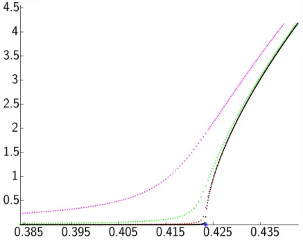
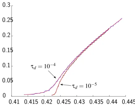
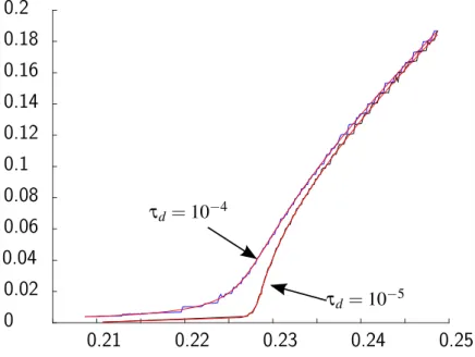
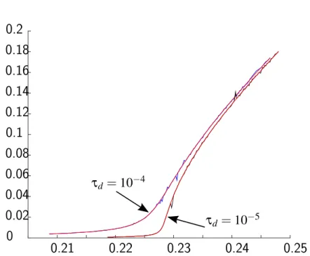
The relevance of this critical ratio for the qualitative analysis of the original system is illustrated by the numerical simulations displayed in Figures 2 to 6. For a given initial condition I0 on the slow variables, we let the drift F0 alone act: We integrate the flow of F0 during a short positive duration τd, then compute the trajectory of the averaged system to go from this point Ipτdq back to to I0. For λ ă λcpI0q, the tensor K is a metric one, and this trajectory is a geodesic. As τd tends to zero, the time τf to come back from Ipτdq tends to zero when λ ă λcpI0q. For λ ě λcpI0q, finitess of this time indicates that global properties of the system still allows to control it although the metric character of the approximation does not hold anymore. (See Figure 2.) The behaviour of τf measures the loss in performance as λ approaches the critical ratio. This critical value depends on the initial condition and gives an asymptotic estimate of whether the thrust dominates the J2effect or not. Beyond the critical value, the system is still controllable, but there is a drastic change in performance. As the original system is approximated by the average one, this behaviour is very precisely reproduced on the value function of the original system for small enough ε. (See Figures 3 to 6.)
References
[1] Agrachev, A. A.; Sachkov, Y. L. Control Theory from the Geometric View-point. Springer, 2004.
[2] Beletsky, V. V. Essays on the motion of celestial bodies. Birkh¨auser, 1999. [3] BepiColombo mission: sci.esa.int/bepicolombo
[4] Bombrun, A.; Pomet, J.-B. The averaged control system of fast oscillating control systems. SIAM J. Control Optim. 51 (2013), no. 3, 2280–2305. [5] Bonnard, B.; Caillau, J.-B. Geodesic flow of the averaged controlled Kepler
Finsler asym´
etrique - E↵et J2
0.385
0.395
0.405
0.415
0.425
0.435
0.5
1
1.5
2
2.5
3
3.5
4
4.5
l
c=
0.4239
l
Cas quelconque. Courbes de
l 7! t
f(l)
pour plusieurs valeurs de
t
d2 {1e 2,1e
3,1e 4,1e 5}
pour le syst`eme moyenn´e.
Figure 2: Value function λ ÞÑ τfpλq, τd Ñ 0 (averaged system). On this example, a “ 30 Mm, e “ 0.5, ω “ Ω “ 0, i “ 51 degrees (strong inclination), and λc » 0.4239. The value function is portrayed for τd“ 1e ´ 2, 1e ´ 3, 1e ´ 4, 1e ´ 5.
[6] Bonnard, B.; Henninger, H.; Nemcova, J.; Pomet, J.-B. Time versus energy in the averaged optimal coplanar Kepler transfer towards circular orbits. Acta Appl. Math.135 (2015), no. 2, 47–80.
[7] Caillau, J.-B.; Cots, O.; Gergaud, J. Differential pathfollowing for regular optimal control problems. Optim. Methods Softw. 27 (2012), no. 2, 177–196. [8] Caillau, J.-B.; Daoud, B. Minimum time control of the restricted
three-body problem. SIAM J. Control Optim. 50 (2012), no. 6, 3178–3202. [9] Caillau, J.-B.; Dargent, T.; Nicolau, F. Approximation by filtering in
opti-mal control and applications. IFAC PapersOnLine 50 (2017), no. 1, 1649– 1654. Proceedings of the 20th IFAC world congress, Toulouse, July 2017. [10] Caillau, J.-B.; Farr´es, A. On local optima in minimum time control of
the restricted three-body problem. Recent Advances in Celestial and Space Mechanics, 209–302, Mathematics for industry 23, Springer, 2016. [11] Caillau, J.-B.; Noailles, J. Coplanar control of a satellite around the Earth.
ESAIM Control Optim. and Calc. Var.6 (2001), 239–258.
[12] A brief introduction to Finsler geometry. Course notes, 2006. math.aalto. fi/~fdahl/finsler/finsler.pdf
[13] Dargent, T.; Nicolau, F.; Pomet, J.-B. Periodic averaging with a second order integral error. IFAC PapersOnLine 50 (2017), no. 1, 2892–2897. Pro-ceedings of the 20th IFAC world congress, Toulouse, July 2017.
Metric approximation of minimum time control systems 10
Finsler asym´
etrique - E↵et J2
0.41 0.415 0.42 0.425 0.43 0.435 0.44 0.445
0
0.05
0.1
0.15
0.2
0.25
0.3
t
fNon averaged
e = 10
3t
fAveraged
l
t
d=
10
5t
d=
10
4l
c=
0.42386
Cas quelconque. Superposition des courbes
l ! t
fpour le syst`eme moyenn´e et
le syst`eme non moyenn´e avec
e = 10
3et
t
d2 {1e 4,1e 5}
. L’extr´emale non
moyenn´ee est choisie telle que son temps final est proche du temps moyenn´e.
Figure 3: Value function λ ÞÑ τfpλq, τd Ñ 0 (original system, ε “ 1e ´ 3). On this example, a “ 30 Mm, e “ 0.5, ω “ Ω “ 0, i “ 51 degrees (strong inclination), and λc » 0.4239. The behaviour of the value function for the original system matches very precisely the behaviour of the averaged one. (See also Figure 4 for a even lower value of ε.)
[14] Edelbaum, T. N. Optimal low-thrust rendez-vous and station keeping, AIAA J.2 (1964), no. 7, pp. 1196–1201.
[15] Geffroy, S.; Epenoy, R. Optimal low-thrust transfers with constraints. Gen-eralization of averaging techniques. Acta Astronaut. 41 (1997), no. 3, 133– 149.
[16] Hampath software: hampath.org
Finsler asym´
etrique - E↵et J2
0.41 0.415 0.42 0.425 0.43 0.435 0.44 0.445
0
0.05
0.1
0.15
0.2
0.25
t
fNon averaged
e = 10
4t
fAveraged
l
t
d=
10
5t
d=
10
4l
c=
0.42386
Cas quelconque. Superposition des courbes
l ! t
fpour le syst`eme moyenn´e et
le syst`eme non moyenn´e avec
e = 10
4et
t
d2 {1e 4,1e 5}
. L’extr´emale non
moyenn´ee est choisie telle que son temps final est proche du temps moyenn´e.
Figure 4: Value function λ ÞÑ τfpλq, τd Ñ 0 (original system, ε “ 1e ´ 4). On this example, a “ 30 Mm, e “ 0.5, ω “ Ω “ 0, i “ 51 degrees (strong inclination), and λc » 0.4239. The behaviour of the value function for the original system matches very precisely the behaviour of the averaged one.
Finsler asym´
etrique - E↵et J2
0.21
0.22
0.23
0.24
0.25
0
0.02
0.04
0.06
0.08
0.1
0.12
0.14
0.16
0.18
0.2
t
d=
10
4t
d=
10
5l
t
f(l)
: Averaged
t
f(l)
: Non averaged,
e = 10
3Cas MEO. Superposition des courbes
l ! t
fpour le syst`eme moyenn´e et le syst`eme
non moyenn´e avec
e = 10
3et
t
d2 {1e 4,1e 5}
. L’extr´emale non moyenn´ee est
choisie telle que son temps final est proche du temps moyenn´e.
Figure 5: Value function λ ÞÑ τfpλq, τd Ñ 0 (original system, ε “ 1e ´ 3). On this example, a “ 11.675 Mm, e “ 0.75, ω “ Ω “ 0, i “ 7 degrees (weak inclination), and λc » 0.2287. The behaviour of the value function for the original system matches very precisely the behaviour of the averaged one. (See also Figure 6 for a even lower value of ε.)
Metric approximation of minimum time control systems 12
Finsler asym´
etrique - E↵et J2
0.21
0.22
0.23
0.24
0.25
0
0.02
0.04
0.06
0.08
0.1
0.12
0.14
0.16
0.18
0.2
l
t
d=
10
5t
d=
10
4t
f(l)
: Averaged
t
f(l)
: Non averaged,
e = 10
4Cas MEO. Superposition des courbes
l ! t
fpour le syst`eme moyenn´e et le syst`eme
non moyenn´e avec
e = 10
4et
t
d2 {1e 4,1e 5}
. L’extr´emale non moyenn´ee est
choisie telle que son temps final est proche du temps moyenn´e.
Figure 6: Value function λ ÞÑ τfpλq, τd Ñ 0 (original system, ε “ 1e ´ 3). On this example, a “ 11.675 Mm, e “ 0.75, ω “ Ω “ 0, i “ 7 degrees (weak inclination), and λc » 0.2287. The behaviour of the value function for the original system matches very precisely the behaviour of the averaged one.