An alternative class of distortion operators

HAL Id: halshs-01543251

https://halshs.archives-ouvertes.fr/halshs-01543251

Submitted on 20 Jun 2017

An alternative class of distortion operators

Dominique Guegan, Bertrand Hassani, Kehan Li

To cite this version:

Dominique Guegan, Bertrand Hassani, Kehan Li. An alternative class of distortion operators :

alter-native tools to generate asymmetrical multimodal distributions. 2017. �halshs-01543251�

Documents de Travail du

Centre d’Economie de la Sorbonne

An alternative class of distortion operators

Alternative tools to generate asymmetrical

multimodal distributions

Dominique G

Bertrand H

Kehan

L

(will be inserted by the editor)

An alternative class of distortion operators

alternative tools to generate asymmetrical multimodal

distributions

Dominique Gu´egan · Bertrand Hassani · Kehan Li

Received: date / Accepted: date

Abstract The distortion operator proposed by Wang (2000) has been devel-oped in the actuarial literature and that are now part of the risk measurement tools inventory available for practitioners in finance and insurance. In this arti-cle, we propose an alternative class of distortion operators with explicit analyt-ical inverse mapping. The distortion operators are based on tangent function allowing to transform a symmetrical unimodal distribution to an asymmetrical multimodal distribution.

Keywords Distortion operator · Multimodal distribution · Asymmetry · Invertibility

JEL classification C20 · G32

1 Introduction

To integrate financial and actuarial insurance pricing theories, Wang (2000) proposes a form of insurance risk pricing based on the standard Gaussian cu-mulative distribution function (cdf) distortion operator with one parameter. He points out that this operator is either concave (when the parameter is D. Gu´egan

Universit´e Paris 1 Panth´eon-Sorbonne, CES UMR 8174, 106 bd l’Hopital 75013; Labex Refi, Paris, France.

E-mail: dominique.guegan@univ-paris1.fr B. Hassani

Universit´e Paris 1 Panth´eon-Sorbonne, CES UMR 8174, 106 bd l’Hopital 75013; Labex Refi, Paris, France.

E-mail: bertrand.hassani@gmail.com K. Li

Universit´e Paris 1 Panth´eon-Sorbonne, CES UMR 8174, 106 bd l’Hopital 75013; Labex Refi, Paris, France.

positive) or convex (when the parameter is negative). Hamada and Sherris (2003) suggests that this operator can shift the quantile of a distribution to the left, thereby assigning higher probabilities to low outcomes. A number of papers propose applications of distortion operators. For example, H¨arlimann (2004) obtains an optimal economic capital formula, under suitable assump-tions on insurance market prices, the collection of possible losses, and the distortion function. Lin and Cox (2005) successfully applies Wang transform to price mortality risk bonds. Hamada et al. (2006) shows a formal treat-ment of risk measures based on distortion functions in discrete-time setting. They conclude that the risk neutral computational approach is well adapted to portfolio optimisation with such measures that do not lie within the ex-pected utility framework. De Jong and Marshall (2007) provides a method for analysing and projecting mortality based on the Wang Transform. Denuit et al. (2007) designs the survivor bonds with the help of Wang transform (Wang (2000)) which could be issued directly by insurers.

However, Godin et al. (2012) argues that it is a well-known fact that the re-turns of most financial assets have semi-heavy tails. Consequently he recognizes that a downside of the normal distortion of Wang (2000) is its underlying sym-metrical that poses some constraints in applications. More precisely, Gu´egan and Hassani (2015) criticize that Wang (2000) applies the same perspective of preference to quantify the risk associated to gain and risk. Thus, the risk manager evaluates the risk associated to the upside and downside risks with the same function that implies a symmetrical consideration for the two effects due to the distortion.

Accordingly, a number of papers make proposals on how to avoid the problem of symmetry in the previous distortion operators. For example, van der Hoek and Sherris (2001) proposes to use two different distortion functions g(x) and h(x) (for instance when g(x) is concave, a convex h(x) = 1 − g(1 − x) would be one possible choice), to allow a different treatment of the upside and downside of the risk. In Wang (2004) a Student-t distribution based distortion operator is introduced allowing for skewness. Sereda et al. (2010) proposes to use two different functions issued from the same polynomial with different coefficients. Godin (2012) introduces a distortion operator based on the Normal Inverse Gaussian (NIG) distribution, which can asymmetrically distort the underly-ing distribution. Gu´egan and Hassani (2015) suggests the use of an inverse S-shaped polynomial function of degree 3 as a distortion operator to create an asymmetrical distribution. Additionally this operator can have a concave part and a convex part by varying its parameters.

Wirch and Hardy(1999) concludes that there is an interest in investigating measures for capital adequacy that utilise the shape of the loss distribution, particularly in the right tail. Specifically, multimodality is one of the impor-tant characteristics of probability distribution. A number of papers related to the income distribution find evidence of multimodality (for a review, see, e.g.,

Bianchi (1997), Jones (1997), Quah (1996a, 1996b, 1997) and Zhu (2005)), for instance the results of Zhu (2005) indicate that the US personal income distribution has been multimodal in 1962, 1972, 1982, 1992 and 2000. Also, he suggests that changes in the shape of the income distribution over the entire income range provide rich information and shed light on issues of income in-equality, poverty traps and convergence. Moreover, he argues that theoretical models should be capable of explaining and generating multimodal income distributions.

Importantly, motivated by the crisis, the multimodal characteristic of distri-butions of some economic variables, for example some stock market indexes like S&P 500 index (the Standard & Poor’s 500), SHCOMP index (Shang-hai Stock Exchange Composite Index) and FTSE Index (the Financial Time Stock Exchange 100 Index), can include useful information of systemic risk. Accordingly it is necessary to find a model such that it is flexible enough to accommodate various shapes of continuous distributions with leptokurtic, skewed and multimodal characteristics.

Additionally, the financial industry has extensively used quantile-based down-side risk measures based on the Value-at-Risk (V aR). In actuarial terms, V aR is a quantile reserve, often using the pth_{percentile of the loss distribution. We}

should emphasize that when we compute the V aR, the explicit analytical form of the inverse mapping of cdf is crucial. Consequently, we propose an alterna-tive class of distortion operators allowing to build an asymmetrical multimodal distribution, with explicit analytical inverse mapping.

We proceed as follows. Section 2 describes the definition and some basic prop-erties of distortion operators. Section 3 presents our model. Section 4 assess the properties of three distortion operators by simulation. Section 5 concludes.

2 Distortion operator

For a continuous distribution with cdf F (f is its probability density func-tion (pdf)), we recall the definifunc-tions of distorfunc-tion operator and multimodal distribution.

Definition 1 (Distortion operator) From Wang (2000), a mapping g: [0, 1] → [0, 1] is a distortion operator if: g is continuous and increasing; g(0) = 0 and g(1) = 1.

Definition 2 (Multimodal distribution) We call F a multimodal distri-bution if its pdf f has multiple local maxima.

Definition 3 (Changing point of concave-convex property) A point x0∈ (0, 1) is called a changing point of concave-convex property for a

distor-tion operator g if g00(x0) = 0, g00(x) < 0 when x ∈ [0, x0) and g00(x) > 0 when

x ∈ (x0, 1].

In his article Wang (2000) specifies that the distortion operator g can be applied to any distributions. A distortion operator g can always transform a cdf F to another cdf g ◦ F (denotes the composition function of g and F ). Denoting Φ the cdf of the standard Gaussian distribution with mean 0 and variance 1 (N(0,1)), Wang (2000) proposes a distortion operator gW as follows:

gW(x) = Φ[Φ−1(x) + a], x ∈ [0, 1] (1)

By illustrating the impact of gW on the logistic distribution, Gu´egan and

Hassani (2015) observes the shift of the mode of the initial distribution only. Further more the close form of gW is not straightforward.

To create multi-modal distributions g ◦ F , assuming f is differentiable and g is twice differentiable, we can derive its associated pdf (g ◦ F (x))0 _{= (g(F (x)))}0₌

g0(F (x))f (x) and

(g ◦ F (x))00= g00(F (x))f2(x) + g0(F (x))f0(x). (2) By definition, g0(F (x)) is always positive. Thus to add hump in (g ◦ F (x))0for a given F , we need to manipulate the sign of g00(F (x)). Consequently concave-convex property of g need to be considered.

Gu´egan and Hassani (2015) provides an inverse S-shaped polynomial function of degree 3 given by the following equation and characterized by a location parameter δ and a shape parameter β

gp(x) = a[ x3 6 − δ 2x 2_{+ (}δ2 2 + β)x], x ∈ [0, 1] (3) where a = (1₆−δ 2+ δ2 2+β)

−1_{, δ ∈ [0, 1] and β ∈ R. They remark that g}

p’s curve

exhibits a concave part and a convex part. We can derive that g00= a(x − δ). Thus when F (x) = δ, g00(F (x)) equals to 0. However, the sign of g00(F (x)) depends on the sign of a, for F (x) ∈ [0, δ) and F (x) ∈ (δ, 1]. Consequently to locate the changing point of concave-convex property of g by δ is confusing.

3 A new class of distortion operators

Property 1 It is twice differentiable. It contains a changing point of concave-convex property x0, with a location parameter to locate x0 and with a shape

parameter to control the concave-convex level of g (characterised by |g00|: the absolute value of g00). Furthermore the inverse mapping of g has a straightfor-ward closed-form.

In order to construct a g satisfying Property 1, first we construct a distortion operator g1by tangent function (since tan(x), x ∈ (−π₂,π₂) is a smooth

func-tion (it has derivatives of all orders) containing x0, and its inverse mapping is

arctan(x))

Definition 4 (Distortion operator g1) For x ∈ [0, 1] with a shape

param-eter 0 < a < π g1(x) = 1 2tana₂(tan(ax − a 2) + tan a 2) (4)

The first and second derivatives of g1 are

g₁0(x) = a 2tana₂ 1 cos2_{(ax −}a 2) (5) g00(x) = a 2 tana₂tan(ax − a 2) (6)

The inverse mapping of g1(x) is

g−1₁ (x) = 1 2 + 1 aarctan(2xtan a 2 − tan a 2) (7)

One can verify that g1(x) is a distortion operator and it has x0=1₂. Thus the

concave-convex property of g1 is symmetrical.

Comparing with Property 1 for g1, a location parameter to locate x0is needed,

which allows g1 to have an asymmetrical concave-convex property.

Definition 5 (Distortion operator g2) For x ∈ [0, 1] with shape parameter

0 < a < π and location parameter b ∈ (1

2, ∞)        g2(x) = 1 2btana₂tan(abx − a 2) + 1 2b, 0 ≤ x ≤ 1 2b g2(x) = 2b − 1 2btana₂tan( ab 2b − 1x + a 2 − 4b) + 1 2b, 1 2b < x ≤ 1 (8)

One can verify that g2 satisfies all conditions in Property 1, whose first and

       g0₂(x) = a atana₂ 1 cos2_{(abx −}a 2) , 0 ≤ x ≤ 1 2b g0₂(x) = a atana 2 1 cos2₍ ab 2b−1x + a 2−4b) , 1 2b < x ≤ 1 (9)          g200= a2_b tana₂tan(abx − a 2), 0 ≤ x ≤ 1 2b g₂00= a 2_b (2b − 1)tana₂tan( ab 2b − 1x + a 2 − 4b), 1 2b < x ≤ 1 (10)

The inverse mapping of g2 is

     g₂−1= 1 abarctan(2bxtan a 2 − tan a 2) + 1 2b, 0 ≤ x ≤ 1 2b g₂−1=2b − 1 ab arctan( 2btana₂ 2b − 1x − tana₂ 2b − 1) + 1 2b, 1 2b < x ≤ 1 (11) 4 Simulation

In this section, first we show the evolution of gp, g1and g2w.r.t (with respect

to) different values of their parameters by simulation (gp is the benchmark),

which allows to compare these distortion operators and remark the difference of two properties of them: concave-convex property level and location of x0.

Second g2 is applied to transform a unimodal F to a multimodal g2◦ F . We

plot the pdf associated to g2◦ F to check the influence of g2.

4.1 Evolution of distortion operators

Firstly we check the concave-convex level of gp, g1 and g2 affected by the

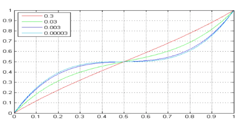
shape parameter. Thus we always fix the location parameter. In Fig. 1, the value of δ is given by 0.5, then we plot the function gp for different values

of β (β = 0.00003, 0.003, 0.03, 0.3). The purpose of Fig. 1 is to show how β can effect the concave-convex level of gp. We observe in this picture that the

curve has symmetrical concave and convex parts, and low values of β are cor-responding to high concave-convex level.

For g1, to understand the influence of the parameter a on the shape of curve,

we plot g1 for a = 0.1π, 0.8π, 0.9π, 0.95π in Fig. 2. The curves show that the

function g1 is always symmetrical. We observe that if a tends to 0 then g1

tends to the identity mapping and when a tends to π the curve exhibits higher concave-convex level.

Fig. 1 Curves of the distortion function gpintroduced in equation (3) for several value of

β (β = 0.00003, 0.003, 0.03, 0.3 and fixed value of δ = 1₂.

Fig. 2 we plot g1in equation (4) for a = 0.1π, 0.8π, 0.9π, 0.95π.

Fig. 3 illustrates the effect of the shape parameter a on g2 using the same

values of a as in Fig. 2 and fixed b = 1. We observe that the curve is sym-metrical and in this case the shape parameter has the same effects as in Fig. 2. Secondly we check the effects of location parameters of gp and g2on the

loca-tion of x0. The location of x0 characterises the asymmetrical concave-convex

property of distortion operators.

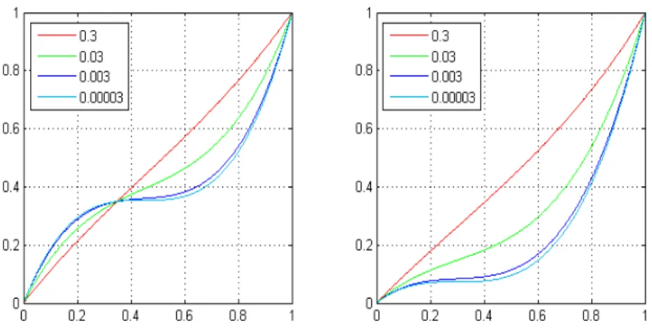
For gp, to illustrate the role of δ on the location of x0, we use two graphs

in Fig. 4. The left graph corresponds to the curve of gp for δ = 0.45 and

Fig. 3 we plot g2in equation (8) for a = 0.1π, 0.8π, 0.9π, 0.95π and fixed b = 1.

δ = 0.3 and β = 0.00003, 0.003, 0.03, 0.3. We observe that through δ one can indeed manipulate the location of x0, but the relationship of them are

confus-ing.

Fig. 4 The left graph corresponds to the curve of gp for δ = 0.45 and β =

0.00003, 0.003, 0.03, 0.3. The right graph provides the curve of gp for δ = 0.3 and β =

0.00003, 0.003, 0.03, 0.3.

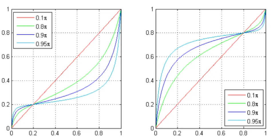
For g2, to understand the influence of the parameter b on the location of x0,

we provide two graphs in Fig. 5. The left graph corresponds to the curve of g2

for b = 2.5 and a = 0.1π, 0.8π, 0.9π, 0.95π. The right graph provides the curve of g2 for = 5₈ and a = 0.1π, 0.8π, 0.9π, 0.95π. We observe the location of x0 is

exactly _2b1.

Fig. 5 The left graph corresponds to the curve of g2 for b = 2.5 and a =

0.1π, 0.8π, 0.9π, 0.95π. The right graph provides the curve of g2 for = 5₈ and a =

0.1π, 0.8π, 0.9π, 0.95π.

From the argumentation and simulation above, we can summarize that g2

meets all the conditions in Property 1.

4.2 Transform a unimodal distribution to a multimodal distribution

To explain how to use g2to transform a given unimodal F to a new

asymmet-rical multimodal g2◦ F , we begin with the N(0,1) with cdf FG and pdf fG.

By plotting the pdf of N(0,1) and the distorted density g20(FG(x))fG(x) with

fixed b = 1 and a = 0.5π, 0.8π, 0.9π, 0.99π, Fig. 6 shows the effect of shape pa-rameter a of g2 on N(0,1). For b = 1, g20(FG(x))fG(x) are always symmetrical.

As a increases, g0₂(FG(x))fG(x) associates a small probability in the centre of

the distribution and puts bigger weight in the tails. We observe two humps in the distorted density when a is large enough.

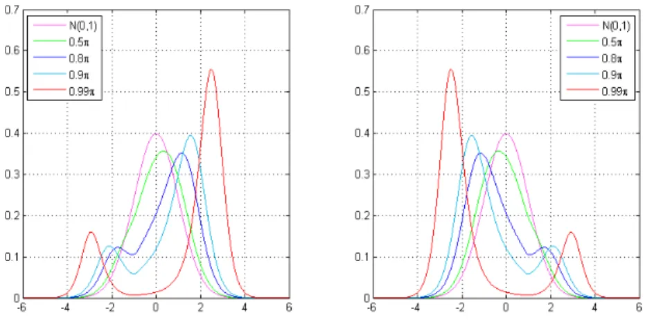
To investigate how the location parameter b of g2 introduces asymmetrical

property into g₂0(FG(x))fG(x), we provide two graphs in Fig. 7 using the same

values of the shape parameters than those used in Fig. 6, but b is 2.5 for the left graph and b is 5₈ for the right one. From Fig. 7 we can remark that the values of a control the information under the humps and the values of b con-trol the locations of the humps. When b 6= 1, g0₂(FG(x))fG(x) is asymmetrical.

Fig. 6 We plot the pdf of N(0,1) and distorted density g0₂(FG(x))fG(x) with fixed b = 1

and a = 0.5π, 0.8π, 0.9π, 0.99π.

high hump of the distorted density is in the right tail for the high value of b in g2; the relatively high hump of the distorted density is in the left tail for

the low value of b in g2.

Fig. 7 The left graph corresponds to the curves of g0₂(FG(x))fG(x) for b = 2, 5 and a =

0.5π, 0.8π, 0.9π, 0.99π. The right graph provides the curves of g02(FG(x))fG(x) for b =58 and

a = 0.5π, 0.8π, 0.9π, 0.99π.

Besides assessing the location parameter b with F coming from the symmet-rical, thin-tail distribution from the elliptical distribution family, it is also necessary to check the influence of b with F coming from the asymmetrical,

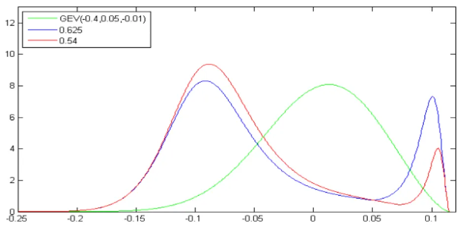
fat-tail distribution. Let FE(fEthe associated density) be GEV(0.2,0.05,-0.01)

(Generalized extreme value distribution with shape parameter k = −0.4, scale parameter σ = 0.05 and location parameter µ = −0.01.). Using the same value of the shape parameter a = 0.95π but different location parameters b = 0.625, 0.54, we plot the distorted density g0

2(FE(x))fE(x) in Fig. 8.

Un-expectedly, instead of controlling the locations of the humps, we observe b controls the information under the humps. Especially lower value of b is asso-ciated to higher left hump and lower right hump.

Fig. 8 Using the same value of the shape parameter a = 0.95π but different location parameters b = 0.625, 0.54, we plot the distorted density g₂0(FE(x))fE(x).

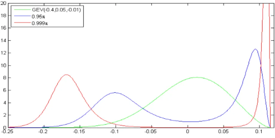
To check if parameter a can affect the locations of the humps or not, we plot the pdf of GEV(0.2,0.05,-0.01) and g0₂(FE(x))fE(x) with the same b = 1 but

different a = 0.95π, 0.999π in Fig. 9. The graph suggests that the parameter a indeed effects the locations of the humps. We observe that the left hump shifts to the left when a increases. It is important to point out that in this simulation, the concave-convex property of g2 is symmetrical since b = 1.

Motivated by Fig. 9, we plot the pdf of GEV(0.2,0.05,-0.01) and g₁0(FE(x))fE(x)

in Fig. 10 using the same values of the shape parameters than those used in Fig. 9. Comparing Fig. 9 and Fig. 10, we observe the same result. Consequently, we can remark that when the original distribution is asymmetrical, it is enough to use g1 if the main purpose is to create an asymmetrical distorted density

with two humps, which possesses the flexibility of shifting the positions of the humps.

Fig. 9 We plot g₂0(FE(x))fE(x) with the same b = 1 but different a = 0.95π, 0.999π.

Fig. 10 We plot g0

1(FE(x))fE(x) using the same values of the shape parameters than those

used in Fig. 9., i.e. a = 0.95π, 0.999π.

5 Conclusion

In this article, we propose an alternative class of distortion operators with explicit analytical inverse mapping. The distortion operators are based on tangent function allowing to transform a symmetrical unimodal distribution to an asymmetrical multimodal distribution.

More precisely, when the original distribution is symmetrical, the first distor-tion operator with just shape parameter can only generate symmetrical dis-torted density. Its shape parameter controls the information under the humps. Consequently, to introduce asymmetry into the distorted density in this case,

it is necessary to use the second distortion operator with both shape parame-ter and location parameparame-ter. Especially, the values of shape parameparame-ter control the information under the humps and the values of location parameter control the locations of the humps.

However, when the original distribution is asymmetrical, unexpectedly we ob-serve that instead of controlling the locations of the humps, the location pa-rameter of the second distortion operator controls the information under the humps. Further more, in this case its shape parameter indeed effect the loca-tions of the humps. Additionally we remark that it is enough to use the first distortion operator which is more concise, if the main purpose is to create an asymmetrical distorted density with more than one humps from an asymmet-rical original density, and at the same time possess the flexibility of shifting the positions of the humps.

6 Acknowledgments

This work was achieved through the Laboratory of Excellence on Finan-cial Regulation (Labex ReFi) supported by PRES heSam under the refer-ence ANR10LABX0095. It benefited from a French government support man-aged by the National Research Agency (ANR) within the project Investisse-ments d’Avenir Paris Nouveaux Mondes (investInvestisse-ments for the future Paris New Worlds) under the reference ANR11IDEX000602.

References

1. Bianchi M (1997) Testing for Convergence: Evidence from Non-parametric Multimodality Tests. Journal of Applied Econometrics 12: 393-409

2. Denuit M, Devolder P, Goderniaux A (2007) Securitization of Longevity Risk: Pricing Survivor Bonds with Wang Transform in the Lee-Carter Framework. The Journal of Risk and Insurance 2007: 87-113

3. Godin F, Mayoral S, Morales M (2012) Contingent claim pricing using a Normal Inverse Gaussian probability distortion operator. The Journal of Risk and Insurance 79: 841-866 4. Gu´egan D, Hassani B (2015) Distortion Risk Measure or the Transformation of Unimodal Distributions into Multimodal Functions. In: Bensoussan A, Gu´egan D, Tapiero C (ed) Future Perspective in Risk Models and Finance, 1st edn. Springer International Publishing, New York, pp 71-88

5. Hamada M, Sherris M (2003) Contingent claim pricing using probability distortion op-erators: methods from insurance risk pricing and their relationship to financial theory. Applied Mathematical Finance 10: 19-47

6. Hamada M, Sherris M, van der Hoek J (2006) Dynamic Portfolio Allocation, the Dual Theory of Choice and Probability Distortion Functions. ASTIN Bulletin 36: 187-217 7. H¨arlimann W (2004) Distortion risk measures and economic capital. North American

Actuarial Journal 8: 86-95

8. van der Hoek J, Sherris M (2001) A class of non-expected utility risk measures and implications for asset allocations. Insurance: Mathematics and Economics 28: 69-82.

9. Jones CI (1997) On the Evolution of the World Income Distribution. Journal of Economic Perspectives 11: 19-36

10. de Jong P, Marshall C (2007) Mortality Projection Based on the Wang Transform. ASTIN Bulletin 37: 149-161

11. Lin Y, Cox SH (2005) Securitization of Mortality Risks in Life Annuities. Journal of Risk and Insurance 72: 227-252

12. Quah DT (1996a) Twin Peaks: Growth and Convergence in Models of Distribution Dy-namics. Economic Journal 106: 1045-1055

13. Quah DT (1996b) Empirics for Economic Growth and Convergence. European Economic Review 40: 1353-1375

14. Quah DT (1997) Empirics for Growth and Distribution: Stratification, Polarization, and Convergence Clubs. Journal of Economic Growth 2: 27-59

15. Sereda EN, Bronshtein EM, Rachev ST, Fabozzi FJ, Sun W, Stoyanov SV (2010) Dis-tortion risk measures in portfolio optimization. In: Guerard JB (Ed), Handbook of Portfo-lio Construction: Contemporary Applications of Markowitz Techniques, Springer US, pp 649–673

16. Wang SS (2000) A Class of Distortion Operators for Pricing Financial and Insurance Risks. The Journal of Risk and Insurance 67: 15-36

17. Wang SS (2004) CAT Bond Pricing Using Probability Transforms. Geneva papers: Etudes et Dossiers 278: 19-29

18. Wirch JR, Hardy MR (1999) Synthesis of risk measures for capital adequacy. Insurance: Mathematics and Economics 25: 337–347

19. Zhu F (2005) A nonparametric analysis of the shape dynamics of the US personal income distribution: 1962-2000. BIS Working Papers 184. http://www.bis.org/publ/work184.pdf