HAL Id: cea-01588251
https://hal-cea.archives-ouvertes.fr/cea-01588251v2
Submitted on 19 Sep 2017HAL is a multi-disciplinary open access archive for the deposit and dissemination of sci-entific research documents, whether they are pub-lished or not. The documents may come from teaching and research institutions in France or abroad, or from public or private research centers.
L’archive ouverte pluridisciplinaire HAL, est destinée au dépôt et à la diffusion de documents scientifiques de niveau recherche, publiés ou non, émanant des établissements d’enseignement et de recherche français ou étrangers, des laboratoires publics ou privés.
Distributed under a Creative Commons Attribution| 4.0 International License
Optical tracking of relaxation dynamics in semi-dilute
hydroxypropylcellulose solutions as a precise phase
transition probe
Hernan Garate, King-Wo Li, Denis Bouyer, Patrick Guenoun
To cite this version:
Hernan Garate, King-Wo Li, Denis Bouyer, Patrick Guenoun. Optical tracking of relaxation dynamics in semi-dilute hydroxypropylcellulose solutions as a precise phase transition probe. Soft Matter, Royal Society of Chemistry, 2017, 13, pp.7161-7171. �10.1016/S0375-9601(99)00347-3�. �cea-01588251v2�
Optical tracking of relaxation dynamics in semi-dilute
hydroxypropylcellulose solutions as a precise phase transition
probe
Hernan Garate*a, King-Wo Li b, Denis Bouyer b and Patrick Guenoun*a
a LIONS, NIMBE, CEA, CNRS, Université Paris-Saclay, CEA-Saclay, 91191 CEDEX
Gif-sur-Yvette, France. *E-mail: hernan.garate@cea.fr (H.G.), patrick.guenoun@cea.fr (P.G.)
b IEM (Institut Européen des Membranes), UMR5635 (CNRS-ENSCM-UM), Université de
Montpellier, Place E. Bataillon, F-34095 Montpellier, France
Abstract
Phase separation of thermo-responsive polymers in solution is a complex process, whose
understanding is essential to screen and design materials with diverse technological
applications. Here we report on a method based on dynamic light scattering (DLS) experiments
to investigate the phase separation of thermo-responsive polymer solutions and precisely define
the transition temperature (TPS). Our results are applied on hydroxypropylcellulose (HPC)
solutions as an important biosourced green water-soluble polymer. As determined by DLS, the
amplitudes of the fast and slow modes of relaxation dynamics evolve as temperature gets closer
to the phase transition point eventually leading to phase separation. The evolution of the modes with temperature is markedly different for concentrations below the overlap concentration (𝑐∗) (dilute regime), above 𝑐∗ (semi-dilute regime) and above the entanglement concentration (𝑐
𝑒). In the three cases though, the fast and slow mode amplitudes undergo a sharp transition in a
narrow temperature range, defining accurately the phase separation locus. The results agree
with turbidimetric analysis for the phase transition determination but with a better precision.
Our results also show that the one-phase dynamics and phase separation dynamics in the
two-phase region are only in continuity for 𝑐 > 𝑐𝑒, revealing mechanistic details about the HPC phase separation process. Above TPS we identify a temperature range where the intensity
growth kinetics of polymer domains and provide clues to rationalize the stabilizing effects of
the interfaces leading to the arrested-like phase separation behavior observed for HPC.
Introduction
Phase separation of thermo-responsive water-soluble polymers is an intense research field in
polymer science driven by promising technologies in a diverse range of fields, among
biomedicine1 and environmentally friendly materials.2-4 Critical aspects to designing and
screening such systems rely on a better understanding of the phase transition and the
determination of well-characterized phase diagrams and phase transition solution temperatures
since the latter temperatures are the main experimental data needed to further investigate the
fundamentals of phase separation mechanisms and kinetics. Different approaches based on
optical measurements (transmittance, scattering intensity at different angles and refractometry)
and differential scanning calorimetry are currently utilized to approach and locate the phase
boundary (TPS) of thermo-responsive water-soluble polymers in a broad range of
concentrations. However, the typical criteria to define such transition are rather arbitrary
without a clear physical significance that justifies a particular choice, which represents one of
the major sources of diversity (as much as 20 % of TPS) of phase diagrams for several
thermo-responsive polymers widely used in applications, such as poly(N-isopropylacrylamide)
(PNIPAm)5, hydroxypropylcellulose (HPC)6,7, methylcellulose8-10, hydroxypropylmethyl
cellulose8,9, among others. Taking into account that phase separation mechanisms of
thermo-responsive polymers strongly depend on the temperature quench depth10 the arbitrariness in
defining TPS represents a clear limitation to investigating phase separation mechanisms and
kinetics in a temperature range close to TPS.
In this article we are interested in exploring another approach to define the phase separation
based on Dynamic Light Scattering (DLS). DLS is a well suited technique to investigate
polymer dynamics over a large concentration range and a large temporal window of relaxation
times.11 In the dilute regime, at which polymer concentration is below the overlap concentration (𝑐∗), the intensity autocorrelation function (𝑔
2(𝑡)) reports a single relaxation mode which describes Brownian motion of single coils for monodisperse systems12 whatever the solvent
quality is.13 At concentrations above 𝑐∗ the system resides in the semi-dilute regime, at which polymer chains overlap and possibly entangle. Li et al. demonstrated that for poly(styrene) in a thermodynamically good solvent (benzene) at 𝑐 𝑐⁄ ∗ = 30, 𝑔
2(𝑡) is still described by a single diffusive relaxation mode,14 while a second non-diffusive relaxation mode is evidenced (slow mode) at higher 𝑡 when the solvent quality gets poorer.13,14 The interpretation of the latter slow mode has been controversial and the subject of extensive research in the last decades for
deciphering its origin with respect to blobs relaxations below or above the entanglement
concentration (𝑐e). Pioneering works by Brown et al.15,16 and more recently Yuan et al.13 attributed the slow mode relaxation to permanent aggregates in the single-phase region, while
more recent experiments11,17 described the slow relaxation dynamics of aqueous PNIPAm
solutions as originating from transient clusters having a non-diffusive nature. In addition, a
second slow dynamical mode was identified for shape-persisitent stiff polymers.18,19 Several
studies in this area focused on the effect of polymer concentration, polymer architecture, and
temperature on the slow mode17,20-22 in order to explain the origin of this slow relaxation
dynamic. Here our goal is different: we address the question of whether it is possible to extract
relevant quantitative information about the phase transition of a polymer solution in the
semi-dilute regime by following the fast and slow mode evolution as temperature gets closer to phase
separation. For this study we selected HPC aqueous solutions as a thermo-responsive
biosourced polymer which was recently designed as an excellent candidate for making porous
temperature behavior in water at 40℃ (up to 40 %),23,24 a very convenient feature for many applications, and was first characterized in 1988 to phase separate by spinodal decomposition at 𝑐 = 10 %.25
In this article we show that the approach of HPC phase transition significantly impacts the fast
and slow mode behaviors. By following the latter modes up to the phase boundary, we
demonstrate that it is possible to define the phase transition temperature with a remarkable
accuracy. This methodology provides a more precise and physically meaningful approach to
determine the phase transition temperature than the commonly used turbidimetric method.
We also show that the evolution of relaxation modes for HPC is strongly concentration
dependent and provides clues to describe the phase separation mechanisms by varying the
concentration. For instance, a remarkable continuity of modes from the single-phase region to
the two-phase region observed for entangled solutions reveals that the non-diffusive transient
clusters formed in the single-phase region are precursors of the phase separating objects.
Finally, we show that DLS can be used to resolve the growth kinetics of HPC domains for
concentrations as high as 5 % and thermal quenches of an amplitude such as the single exponential nature of 𝑔2(𝑡) is preserved.
Experimental
Sample preparation
A commercial HPC (Sigma-Aldrich) was employed for this study since the very same polymer
proved to be a valuable choice for further applications for membranes.3 The weight average
molecular weight (𝑀W), evaluated by size exclusion chromatography (Shimadzu LC-20AD) using a Shodex OHpak SB-803/SB-804 column and poly(ethylene glycol) molecular weight
standards, is 72 kg/mol and PDI3. HPC aqueous solutions in the concentration range 0.5 to 30 % (wt.%) were prepared by fully dispersing HPC powder in preheated Milli-Q water at 60℃
with stirring for 2 h. The samples were then cooled and stored at 4℃ overnight to complete hydration of the polymer. The aqueous solutions were transparent at room temperature.
Samples with 𝑐 ≤ 10 % were filtered using 0.45 m Millipore filters directly into dust-free PMMA light scattering cuvettes. Solutions with concentration higher than 20 % were prepared from filtered 10 % solution and concentrated under reduced pressure (220 mbar) at 60℃ due to the impossibility to filter such concentrated samples. The overlap concentration 𝑐∗ was determined from the definitions 𝑐∗ = 3𝑀/(4𝜋𝑁A𝑅g3), 𝑀/(23/2𝑁A𝑅g3), and [𝜂]−1, where 𝑀, 𝑅g, 𝑁A and [𝜂] are the molar mass, the radius of gyration of polymer chains, the Avogadro constant and the intrinsic viscosity, respectively. In this work we use the 𝑐∗ value obtained from [𝜂]−1, since the other two definitions are less precise due to the uncertainty in 𝑅
g as PDI is
high. The entanglement concentration 𝑐e, representing the concentration above which the polymer chains form an entangled network, was estimated as 𝑐e ≈ 10𝑐∗, as reported by Colby26 for neutral polymers in good solvent conditions. The radius of gyration of polymer chains was determined as 𝑅g= 1.56𝑅h, assuming good solvent conditions far enough from TPS, where 𝑅h
is the hydrodynamic radius calculated from diffusion coefficient D obtained by DLS experiments of diluted samples employing the Stokes-Einstein equation, 𝑅h = (𝑘B𝑇/6𝜋𝜂0)/𝐷, where kB, T and 𝜂0are the Boltzmann constant, the absolute temperature, and the solvent viscosity, respectively. Since the polymer is polydisperse, 𝐷 means actually an average 𝐷 over the size distribution of chains. Intrinsic viscosity was measured by the rolling ball principle
using a microviscometer Lovis 2000M (Anton Paar) at a fixed angle of 85º. HPC solutions were prepared by dilution in the concentration range of 0.01-2 % and measured at 30℃.
Dynamic light scattering
Back-scattering intensity autocorrelation function (𝑔2(𝑡)) was obtained using a Zetasizer Nano ZS (Malvern Instruments Ltd., Worcestershire, UK) (temperature control range 0-90℃, ±
0.1℃) equipped with a 4 mW He-Ne laser of 𝜆o= 633 nm. The angle between the laser beam and the detector (avalanche photodiode) was 𝜃 = 173°and the scattering vector (𝑞) (𝑞 = (4𝜋𝑛 𝜆⁄ ) sin(𝜃 20 ⁄ )) was 0.02633 nm-1. The laser power was automatically attenuated to collect an optimal scattered intensity. The measurement penetration depth into the sample was
set to 2 mm. A 30 s acquisition time was generally enough to obtain a stable intensity
autocorrelation function. Increasing the acquisition time up to 100 times the slower dynamical
mode relaxation time did not provide any additional change in the signal of the intensity
autocorrelation function. HPC solutions were heated at different T in the range between 29.4 and 48℃ in which TPS is found. The heating rate (3 °C min⁄ ) allowed a fast thermal equilibration at each final temperature (equilibration time was measured using a thermocouple
within solution). Measurements in the two-phase region (T˃TPS) were performed either close
to TPS (T − TPS ≤ 4 oC) or well above TPS (T − TPS ≥ 10 oC). The final temperature was reached after 1 min heating in the two-phase region at Tclose to TPS and up to 4 min heating in
the two-phase region at Twell above to TPS. Intensity autocorrelation functions were measured
at different temperatures as a function of time at 5 min time intervals until no significant
differences were observed in consecutive measurements (between 10-30 min). Repeated
measurements were performed at each temperature at 1 h interval to ensure data are in steady state. Before each measurement at a certain temperature, an equilibration step at 29.4℃ for 30 min was performed.
𝑔2(𝑡) can be related to the normalized electric field correlation function 𝑔1(𝑡) by the Siegert relation as12
𝑔2(𝑡) = 𝛽|𝑔1(𝑡)|2 (1) where 0 < 𝛽 < 1 is a constant related to the coherence of the detection optics. For a polydisperse system,27 𝑔
1(𝑡) is related to the distribution of the characteristic relaxation time distribution (𝐺(𝜏)) as
|𝑔1(𝑡)| = ∫ 𝐺(0∞ )𝑒−𝑡/d (2) In this study (𝐺(𝜏)) was calculated using the Laplace inversion of 𝑔1(𝑡) (normalized to 1 at 𝑡 = 0) on the basis of eqs 1 and 2 by the Maximum Entropy Method.12,28 𝐺(𝜏) usually displays two major relaxation modes (fast and slow). Fast mode correlation time (𝜏fm) and slow mode correlation time (𝜏sm) were extracted from the mean peak position of fast and slow relaxation modes, respectively. The contribution of each mode (amplitude) was obtained from the relative
peak area of each distribution mode. Additionally, correlation times and amplitudes were also
obtained by a similar analysis than that reported by Yamamoto et al.20 by fitting to a sum of
single-exponential functions. The obtained results (data not shown) were in good agreement
with those obtained from Maximum Entropy Method.
Turbidimetric measurements
Phase separation temperatures were determined by optical transmittance method using a quartz cell filled with HPC solutions inserted in a thermostat (0.01℃ precision). For determining TPS, a 5 mm thick cell was used, shined by a laser beam (𝜆 = 632.8 nm). Two photodiodes were placed before and after the sample to measure the transmission of the light through the sample. Thermal steps of 0.2℃ followed by 30 min equilibration time were performed to monitor the transmittance versus time. As the temperature approached TPS the transmittance decreased with
time asymptotically, and therefore the transmittance at infinite time 𝜏∞ (T∞) at each thermal step was extrapolated by fitting to 𝑦 = 𝐴1exp(−𝑡 𝑡⁄ )1 + T∞. From transmittance vs temperature curves, TPS was determined by two different criteria: i) As the abscissa of the intercept between the horizontal asymptote at low temperatures and the tangent to the transmission decrease (T_); ii) As the middle point on the slope of variation between 𝜏∞ and 𝜏0 (T1 2⁄ ).
Confocal laser scanning microscopy
HPC phase separation was monitored using an Olympus Fluoview FV1000 inverted confocal
microscope. HPC solution (10 L) was sandwiched between two glass slides separated and sealed by a polydimethylsiloxane ring (200 m thick). Rhodamine 6G Chloride was used as the hydrophilic fluorophore. Micrographs were collected with a 40X objective. A thermal stage (Linkam PE 94) was used to control the temperature. The solutions were equilibrated at 30℃ for 30 min followed by heating to the final quench temperature at a rate of 5℃/min. The working distance of the objective was focused in a plane inside the solution, away (~40 μm) from the cover glass, in order to avoid interface effects.
Results and discussion
The overlap concentration (𝑐∗) was estimated to be 1.2 % as defined in the experimental section. In the dilute regime the product 𝑞. 𝑅g, where q is the scattering vector and 𝑅g the radius of gyration of the polymer, was estimated to be 0.592 (𝑞 = 0.02633 nm−1, 𝑅g = 22 nm) satisfying 𝑞. 𝑅g˂1. Under these experimental conditions the correlation function yields information about the whole macromolecular motion and not about internal motions of single
coils.29 At 𝑐 = 0.5 % the system is in the dilute regime and T
PS was determined to be 44℃ from turbidimetric measurements. The entanglement concentration 𝑐e for aqueous HPC at 30℃ should be close to 10 % based on 𝑐∗ value. Figure 1 shows the intensity-intensity time correlation function 𝑔2(𝑡) variation in the T range between 29.4 and 47.3℃ for HPC aqueous solutions in the dilute regime (𝑐 = 0.5 %) (Figure 1a) and semi-dilute regime above 𝑐e (𝑐 = 20 %) (Figure 1b) collected after 30 min equilibration. By increasing T in a narrow temperature range (42.8-43.8 ℃ at 0.5 % and 36.5-37.6 ℃ at 20 %) the 𝑔2(𝑡) signal presents an abrupt change, corresponding to the phase separation transition. Decay time distribution functions
(𝐺(𝜏)) were obtained from the Laplace inversion by the Maximum Entropy Method. The temperature evolution of 𝐺(𝜏) at different concentrations is presented in Figure 2 where the relaxation time distribution is plotted as a function of 𝜏𝑇 𝜂⁄ at different polymer concentrations 0 and temperatures, where 𝜂0 is the solvent viscosity at each T. This renormalization of time was adopted to suppress trivial thermal dependence not related to phase separation, enabling direct
comparison of peak position at different T.14,15,30
Figure 1. Temperature dependence of intensity autocorrelation function 𝑔2(𝜏) for
concentrations (a) 0.5 % and (b) 20 % at a scattering angle of 173o.
At 𝑐 = 0.5 % 𝐺(𝜏) reports a single relaxation mode (at 𝜏𝑇 𝜂⁄ 0 27 Pa-1K) below 42.8℃, which turns into a single relaxation mode with higher 𝜏𝑇 𝜂⁄ (0 103 Pa-1 K) from 43.8℃, as the polymer phase separates (Figure 2a). It is worth noting that at 𝑐 < 𝑐∗ in the single-phase region (T ≤ 42.8 °C) the distribution observed for the single relaxation mode is rather broad as a result of the polydisperse nature of the biosourced commercial HPC. By increasing 𝑐 to 1 % (roughly at 𝑐∗), turbidimetric analysis estimates a T
PS of 42.7℃. Figure 2b shows that relaxation time distribution at 𝑐 = 1 % displays a principal mode (𝜏𝑇 𝜂⁄ 0 20 Pa-1K) together with a slow
mode of small amplitude at higher 𝜏𝑇 𝜂⁄ (0 100 Pa-1K). Fast and slow modes are almost constant in reduced 𝜏 by increasing T in the range (29.4-41.3)℃. However, in the narrow T range 41.3-43.3℃ around TPS the proportion of the fast and slow mode inverts showing a marked shift in amplitudes downwards and upwards, respectively. Additionally, the slow mode increases in 𝜏𝑇 𝜂⁄ by a noticeable amount at the transition. 0
Figure 2. Relaxation time distribution𝐺(𝜏)at different temperatures for concentrations (a) 0.5 %, (b) 1 %, (c) 5 % and (d) 20 %.
At 𝑐 ≥ 5 % the complexity of 𝐺(𝜏) increases. Two major modes (fast and slow) are observed in combination with a small contribution of a third mode at 𝜏𝑇 𝜂⁄ between fast and slow modes. 0 However, due to the negligible contribution of this third mode, we shall ignore this intermediate
relaxation mode in the following analysis. A first qualitative analysis of relaxation mode evolution with T in the semi-dilute regime indicates that at 𝑐 = 5 % (TPS40℃ by turbidimetry) the fast and slow mode contributions are equivalent and constant with increasing T until a narrow temperature range (39.3-40.1)℃ at which the fast mode decreases to almost zero and the slow mode amplitude increases sharply, as presented in Figure 2c. Moreover, reduced relaxation time of fast mode undergoes a slight shift to higher 𝜏𝑇 𝜂⁄ in the range 29.4-39.8 ℃, 0 while that for the slow mode is roughly constant in the same T range. However, the slow mode undergoes a marked shift to higher 𝜏𝑇 𝜂⁄ in the T range (39.3-40.1) ℃ close to T0 PS.
At 𝑐 = 20 % (Figure 2d) the behavior of the fast mode is similar to that observed at 𝑐 = 5 %, showing a marked shift to higher 𝜏𝑇 𝜂⁄ with increasing T. However, the slow mode now 0 displays a remarkable continuity in 𝜏𝑇 𝜂⁄ in the entire T range analyzed in this study. 0 Interestingly, at all concentrations it is observed that above the temperature range at which the
fast mode vanishes i.e. in the two-phase region, 𝐺(𝜏) turns out to be a single narrow mode related to phase separation under the form of polymer aggregates. Small variations in
normalized 𝜏 at this T range are likely due to the aggregate size dependence on the thermal quench, an effect consistent with previous phase separation studies on HPC25 and PNIPAm.31
Fast mode
When the polymer concentration is below 𝑐∗ the single relaxation mode is attributed to Brownian motion of single coils,12 whereas for concentrations above the overlap concentration (𝑐 > 𝑐∗) this mode reflects cooperative diffusion of chain segments between each blob.32 Figure 3a shows the polymer concentration dependence of fast mode relaxation time at T=29.4
℃. An approximate plateau region is found at concentrations below 0.5 % whereas 𝜏fm decreases more markedly with polymer concentration above 0.5 %. This observation suggests that the solution below 0.5 % is in the dilute regime (𝑐 < 𝑐∗) while at 𝑐 > 1 % the system enters the semi-dilute regime, in agreement with 𝑐∗ estimation (1.2 %). The decrease in 𝜏fm as the polymer concentration increases above 1 % indicates that the average segment correlation
length decreases as concentration increases, following a similar trend as that reported for
PNIPAm.33
Figure 3. (a) Fast mode relaxation time vs. concentration in the single phase region at 29.4℃
and normalized fast mode relaxation time (𝜏fm𝑇 𝜂⁄ ) vs. T for concentrations (b) 0.5 %, (c) 5 0 % and (d) 20 %.
Figures 3b-d display the temperature dependence of the reduced fast mode relaxation time (𝜏fm𝑇 𝜂⁄ 0) at three different concentrations (0.5, 5 and 20 %). As discussed before, when the polymer phase separates by increasing T the slow mode becomes the major distribution and the
fast mode contribution decreases to almost zero. However, in a temperature range above the
transition but close enough to it, the decay time distribution functions obtained by the Maximum
Entropy Method still evidence a small contribution of fast mode that is reported in Figure 3. At 𝑐 = 0.5 %, 𝜏fm𝑇 𝜂⁄ undergoes a slight increase with T up to 0 43℃ above which it displays an abrupt shift to higher values as the fast mode disappears. Reduced relaxation time at 𝑐 = 5 % shows a slight increase with T below 39℃, which becomes more notorious above 39℃, likely due to phase separation (PS) into a polymer rich and a polymer lean phase. However, the latter increment of 𝜏fm𝑇 𝜂⁄ in the two-phase region at 𝑐 = 5 % is notably less marked than that at 0 𝑐 = 0.5 %. On the contrary, at 𝑐 = 20 % the reduced relaxation time 𝜏fm𝑇 𝜂⁄ steadily 0 increases with T, but no sharp transition is observed within the analyzed temperature range. The slight increment of 𝜏fm𝑇 𝜂⁄ observed below PS in the entire concentration range is likely 0 due to the gradual decrease in solvent quality as the temperature increases from 30℃ (relatively good solvent condition) to the vicinity of theta condition (40℃)34 where the interactions between segments and segment-solvent gradually change. Brown et al. showed a similar slight
increase of fast relaxation time for polystyrene semi-dilute solutions from good solvent
(toluene) to theta solvent (2-butanone) conditions, while the fast mode amplitude remained
constant.29 A similar trend was observed by Li et al.14 by cooling polystyrene solution in
cyclohexane. The authors explained these results by considering that when the solvent quality decreases, polymer chains contract, resulting in an increase of 𝑐∗ and therefore a slight shift in fast mode relaxation time to higher values, as shown in Figure 3a. Interestingly, over the entire
concentration range studied here the fast mode amplitude remains constant up to a temperature
show that the temperature variation of the reduced fast mode relaxation time has no clear dependence with the concentration ranges delimited by 𝑐∗or 𝑐
e.
Slow mode
Figure 4a shows the concentration dependence of the reduced slow mode relaxation time (𝜏sm𝑇 𝜂⁄ ) at 29.4℃ in the single phase region and the corresponding amplitude. As the 0 concentration increases, 𝜏sm𝑇 𝜂⁄ is larger and the slow mode amplitude increases. These 0 observations indicate that the slow dynamic process is closely related to chain
clustering/entanglement effects.17 DLS experiments in the forward-scattering configuration at
c = 20 % (θ = 13°; 𝑞2 = 8.925 x 10⁻⁶ nm−2, acquisition time 1000 s) provided values of 𝜏sm= 29.3 s and fast mode amplitude/slow mode amplitude = 0.59, while the corresponding values for back-scattering (θ = 173°; 𝑞2 = 6.9327 x 10⁻⁴ nm−2) were 1.2 s and 1.05, respectively. The plot 1 𝜏⁄ sm vs. 𝑞2 deviates from a straight line passing through the origin, evidencing the non-diffusive nature of the slow mode as previously observed for different
polymer solutions.13 The plots of the slow mode amplitude vs T shown in Figure 4b-f reveal
that at some temperature the amplitude undergoes a sharp transition to higher values in the
entire concentration range between 1 and 30 %. Moreover, the temperature of this transition
decreases with polymer concentration and coincides with the fast mode amplitude transition.
Therefore, we can now rationalize the fast and slow amplitude shifts with increasing
temperature as coinciding with the HPC phase separation transition, where polymer chains
Figure 4. (a) Reduced slow mode relaxation time (𝜏sm𝑇 𝜂⁄ ) and slow mode amplitude vs. 0
concentration in the single-phase region at 29.4℃. Reduced slow mode relaxation time and amplitude dependence on T for concentrations (b) 1%, (c) 10 %, (d) 15 %, (e) 20 % and (f) 30
%. Dotted lines correspond to sigmoidal fittings for amplitude vs T plots.
Note that at 𝑐 ≤ 10 % there is a narrow T range at which 𝜏sm𝑇 𝜂⁄ shifts to larger correlation 0 times, as presented in Figure 4b-d. This temperature range coincides with the temperature at
This behavior is consistent with results by Yamamoto et al.20 for semi-dilute aqueous PNIPAm
solutions showing a sharp transition in slow mode relaxation time at TTPS. However, it is worth highlighting that the slow mode behavior with increasing temperature observed for HPC
is in marked contrast to that reported by Yuan et al. for aqueous PNIPAm in semi-dilute regime,
where the slow mode reduced 𝜏 was observed to become faster by increasing T below TPS.13 This suggests that the slow mode reduced 𝜏 variations with temperature could be dependent on the nature of the thermo-responsive polymer. Remarkably, this behavior is no longer observed for HPC solutions above 𝑐 = 15 % as the reduced 𝜏sm shows a clear continuity before and after phase separation, as presented in Figures 4e,f. In this regard, we suggest that the different T
dependence of 𝜏sm𝑇 𝜂⁄ at 𝑐 ≤ 10 % and at 𝑐 ≥ 15 % is related with the transition between 0 the overlap and entanglement regimes (𝑐e is roughly 10 %). In the non-entangled range (𝑐∗ < 𝑐 ≤ 𝑐e), at which polymer chains overlap to some extent without entanglement formation, the shift of 𝜏sm𝑇 𝜂⁄ to higher values by increasing T at 0 TPS reflects chain and clustering association at the phase separation condition. By contrast, in the entangled range (𝑐 ˃ 𝑐e) the fact that 𝜏sm𝑇 𝜂⁄ is constant below and above T0 PS would imply that no additional or further chain/cluster association occurs during phase separation in this concentration range. This
presumably reflects that the transient clusters present in the single-phase region are precursors
of polymer aggregates formed in the two-phase region. This picture of phase separation of HPC
aqueous solutions at 𝑐 ˃ 𝑐e raises the question of the nature of the molecular organization occurring at the phase separation transition. While the observation that the fast mode amplitude
decreases abruptly at TPS reflects the formation of HPC-HPC contacts/interaction, the almost
identical relaxation dynamics found between the slow mode below TPS and the single mode
above TPS suggest that preformed aggregates in the two-phase region may retain considerable
Phase diagram
From the analysis of fast and slow correlation times and amplitudes it was evidenced that PS
temperatures at different concentrations cannot be obtained by following the evolution of the reduced relaxation times only, in particular at 𝑐 ˃ 𝑐e. Although this approach could be useful in the dilute regime,9 the lack of sharpness in temperature dependence when the concentration is
above 5 % precludes a precise definition of the phase separation transitions.
By contrast, the observed transitions in the fast and slow mode amplitudes could be employed
to precisely map phase separation diagram of HPC in a broad concentration range and this
approach compares favorably to TPS determination obtained by other methods. For comparison,
Figure 5a shows that the phase separation temperatures determined by the fast and slow mode
amplitude evolution with T are identical. The advantage of this approach is that this DLS
analysis conducts to sharp transitions that can be used to accurately define TPS as the temperature at which the fast and slow mode amplitude diverges (experimental error ± 0.3℃). On the other hand, the typical method employed to map phase separation diagrams of HPC,
based on following the drop in transmittance as the polymer phase separates with increasing
temperature, provides a transmittance signal that decreases slowly with T (Figure 5a). The latter
approach prevents a well-defined TPS determination because the transition lacks sufficient
sharpness, reducing the accuracy of the method.6 In fact, this drawback is one of the main
factors contributing to diversity of phase separation diagrams since different criterions can be
selected to determine TPS, as outlined in a recent work of Halperin et al.5 In this regard, a
significant discrepancy (see Figure 3 in Marsano et al.7) was found by comparing previously
reported phase diagrams of aqueous HPCbased on turbidity measurements from HPC with
similar molecular weight and structure for which no discrepancy is expected.6,36 Figure 5b
displays the phase separation diagrams for aqueous HPC solutions in the concentration range 𝑐 = (0.5 − 30)% obtained by DLS from sigmoidal fittings of fast and slow mode amplitude
transitions (red) and turbidimetric analysis taken as the midpoint of the transition (T1 2⁄ ) (green) and by the tangent method (T_) (blue). We found that TPS obtained by DLS are in very good agreement with optical transmittance results T_ but with much smaller error bars for the DLS determination. By contrast, the T1 2⁄ method appears to exceed TPS obtained by DLS at equivalent polymer concentration by an average of 2.0℃ (experimental error ±0.3℃), which becomes even larger at the lowest concentration (T1/2− TPS = 4.5 ℃). However, the general trend of the diagrams is very similar with a pronounced decrease of TPS at 0.5 % < 𝑐 < 1 % and a gradual decrease at 1 % < 𝑐 < 30 %, in agreement with some previous theoretical and experimental HPC phase diagrams reported by Lárez-V et al.37 This approach thanks to DLS
fully clarifies why the so far rather empirical choice of T_as the PS temperature is probably justified but much less precise.
Additional experiments performed on aqueous poly(vinyl)alcohol solutions (10 wt.%) with a
degree of hydrolysis of 72 % also showed good agreement between the TPS obtained by DLS (36℃, data not shown) and the onset of phase separation previously reported by turbidimetric analysis,2 suggesting that the method to track the TPS presented here is probably relevant for
Figure 5. (a) Transmittance, fast and slow mode amplitude temperature dependence for 𝑐 =
20 %. Dotted curves correspond to sigmoidal fittings. (b) Phase diagram of aqueous HPC obtained by DLS and turbidimetry (T_ , T1 2⁄ ) in the range 𝑐 = (0.5 − 30)%.
Insights into the two-phase region
A correct interpretation of 𝑔2(𝑡) in the two-phase region may give access to monitoring the phase separation kinetics and measuring characteristic size of polymer aggregates which may form and grow with time. However, DLS theory can only be applied to interpret 𝑔2(𝑡) signal provided multiple-scattering effects are absent. As HPC aqueous solution enters into the
two-phase region, the system gets turbid (near TPS) and by further heating the sample well above
TPS (T − TPS ≥ 10 oC), it turns into a cloudy phase separated system. Despite this apparent multiple-scattering character above TPS, the correct interpretation of 𝑔2(𝑡) actually depends on the T quench depth. To illustrate this effect, 𝑔2(𝑡) was collected at different temperatures using a heating rate of 3 °C min⁄ to allow for a fast quenching experiment (less than 1 or 4 min heating in the two-phase region for the lower and higher T quench, respectively). Figure 6a shows that 𝑔2(𝑡) signal is mostly a single exponential in the two-phase region near TPS (T − TPS ≤ 4 oC). By contrast, for a higher T quench (T − TPS ≥ 10 oC), 𝑔2(𝑡) deviates from the single exponential behavior, as represented in Figure 6a at the same concentration. This is likely
due to the formation of denser polymer aggregates that act as efficient scatterers bringing
multiple-scattering effects. Indeed, in the multiple-scattering regime, in the back-scattering geometry, 𝑔2(𝑡) can be fitted to Eq. 3 according to diffusing-wave spectroscopy theory (DWS) assuming spherical scatterers.38
𝑔2(𝑡) = 𝑒−2𝛾(6𝑡𝑡0)𝑎 (𝑎 = 0.5) (3)
with 𝛾 = 〈𝑧𝑜〉
𝑙∗ +
2
3, where 2/3 is an empirical fitting parameter, 𝑙
∗ is the transport mean free path
and 〈𝑧𝑜〉 is the average penetration depth into the sample (2 mm in the experiments), 𝑡0 is the characteristic relaxation time and the exponent 𝑎 is 0.5 in DWS theory. The 𝑔2(𝑡) signal was measured as a function of time at 50℃ for concentrations 5, 10 and 20 % and fitted to Eq 3. At 30 min, the best-fitted values of 𝑎 are 0.65, 0.51 and 0.49 (± 0.03) at 5, 10 and 20 %, respectively. Figure 6b displays the logarithm of the normalized autocorrelation function at 𝑐 = 5 %, 10 % and 20 % plotted as a function of (𝑡 𝑡
0
⁄ )𝑎 using the best values of 𝑎.
Figure 6. Log(𝑔2(𝑡)) collected in the back-scattering geometry (173o) after 30 min equilibration. Data is plotted as function of time (a) at 41.3℃ (diamonds) and 50℃ (pentagons)
(𝑐 = 10 %) and as a function of (𝑡 𝑡⁄ )0 𝑎
(b) at 50℃ at concentrations 5 % (squares), 10 % (circles) and 20 % (triangles).
The data are described satisfactorily by Eq. 3 (𝑎 = 0.5) at 𝑐 = 10 % and 20 %, while a slight deviation to a higher a value is encountered for 𝑐 = 5 %.
These results give evidence of the existence of two regimes within the 2-phase region: (1)
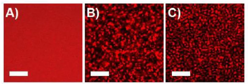
Single-scattering regime, in the T range close to TPS (T − TPS ≤ 4 oC), where the single-exponential nature of 𝑔2(𝑡) is preserved for at least 6 h; (2) Multiple-scattering regime, in the T range well above TPS (T − TPS ≥ 10 oC), presumably by the formation of denser polymer aggregates. Confocal microscopy images taken at 𝑐 = 5 % in both regimes reveal that deeper T (T − TPS ≥ 10 oC) quenches lead to denser structures, as presented in Figure 7, supporting the picture of multiple-scattering regime produced by denser particles.
Figure 7. Confocal scanning microscopy images for 𝑐 = 5 % taken at (a) 30℃ (clear solution),
(b) 43℃ and (c) 50℃ after 30 min equilibration. The red features are attributed to water-rich domains, whereas the darker regions correspond to polymer-rich phases. Scale bar is 20 m.
We now address the question of whether the characteristic size of polymer aggregates can be
estimated in the single-scattering (DLS) and multiple-scattering (DWS) regimes. For
comparison, the average distance (the domain length, 𝑑Confocal) was determined by Fourier transform analysis of confocal microscopy images collected as time elapses at identical quench
temperatures. The diffusion coefficient (D) was obtained from the correlation time of the single mode (𝜏 = 1 𝐷𝑞⁄ 2) above T
PS (single-scattering regime) at different concentrations between 0.5 and 10 %. From 𝐷 values, we estimate the characteristic diameter (𝑑DLS) of aggregates using the Stokes-Einstein relation, assuming spherical shapes of polymer domains and
negligible interactions between them. The estimated aggregate sizes in the single-scattering
regime after 30 min equilibration are in good agreement with 𝑑Confocal for dilute enough solutions (𝑐 ≤ 5 %), as presented in Table 1. However, the large differences observed for concentrated solutions (𝑐 = 10 %) manifest that the diffusion coefficient of the aggregates cannot be interpreted as originating from non-interacting objects and that the diffusion
coefficient deviates from the dilute limit (Stokes-Einstein value).
Table 1. Characteristic HPC domain size in the two-phase region obtained in the concentration
range (0.5-10 %).
*Experimental data of 𝑔2(𝑡) does not fit to Eq. 3
Regarding the multiple-scattering regime, fits of 𝑔2(𝑡) to Eq. 3 assuming a 𝛾 value of 1.33 (non-interacting particles) conducts to significant overestimations of the characteristic domain
size with respect to confocal microscopy analysis, which evidence that the interactions between
polymer aggregates cannot be neglected in the concentration range considered here. It is worth
noting that Sanyal et al.39 showed that 𝛾 decreases with the repulsive interactions between 𝒄 (%) Single-scattering regime(T-TPS = 4℃) Multiple-scattering regime (T-TPS = 10℃) 𝑑DLS(m) 𝑑Confocal(m) 𝑑DWS (m) 𝑑Confocal(m) 0.5 1.5 ± 0.5 3 ± 1 (*) 2 ± 1 1 2 ± 1 4 ± 1 (*) 3 ± 1 5 12 ± 2 10 ± 2 74 ±8(=1.33) 3 ± 1(=0.3) 4 ± 1 10 64 ± 5 9 ± 2 740 ± 80(=1.33) 3 ± 1(=0.1) 3 ± 1
particles and found 𝛾 values as low as 0.1 for strongly interacting systems. By fitting 𝑔2(𝑡) to Eq. 3, assuming that 𝑑DWS= 𝑑Confocal as obtained in the multiple-scattering regime, one gets a 𝛾 value of the order of 0.3 at 𝑐 = 5 % and 0.1 at 𝑐 = 10 %. Although this is consistent with expectations, a precise determination of 𝛾 for HPC at different compositions is clearly out of the scope of this report.
Figure 8a shows the evolution of 𝑑DLS with time at 𝑐 = 5 % (single-scattering regime, 43℃). In the earlier stage of the experiment (𝑡 ≤ 10 min), 𝑑DLS satisfies a scaling law 𝑑DLS(𝑡)~√𝑡3
,
suggesting that HPC domain growth may follow a classical coarsening behavior.25,40 Note that for 𝑡 > 10 min, 𝑑DLS reaches a plateau indicating that further coarsening of polymer domains is impeded. Such arrested phase separation behavior is consistent with the absence of
macroscopic phase separation in the entire concentration range considered in this study (even after 5 days at 43℃). DLS results compare favorably well with the growth kinetics captured by confocal microscopy (Figure 8).
Figure 8. Evolution of characteristic dimension 𝑑DLS and 𝑑Confocal as a function of time during phase separation of HPC solutions at 𝑐 = 5 % in (a) pure water and (b) NaCl 0.01 M.
The arrested-like phase separation behavior observed for other LCST noninonic water-soluble
polymers has been regarded as originating from gelation (methylcellulose,8,10
hydroxypropylmethylcellulose8) or from the effect of electrostatic charges at the interface of
polymer aggregates inducing colloidal stability (PNIPAm31). However, our results show that
HPC phase separation is fundamentally different from those systems since phase separation
does not induce gelation, and the arrested-like behavior after the growing stage persists by
increasing the ionic strength (Figure 8b), which rules out a pure electrostatic effect as for the
case of PNIPAm. In addition, confocal microscopy analysis revealed that the arrested phase separation behavior is also observed for higher T quenches (50℃, data not shown) where the multiple-scattering regime is relevant. A potential explanation to the observed HPC
arrested-like phase separation mechanism could be the formation of polymer aggregates concentrated
enough (glassy) to prevent colloidal coalescence. However, validation of this hypothesis would
require direct measuring of the aggregate composition, and is left for a future work.
Conclusions
The thermo-responsive phase separation of commercial hydroxypropylcellulose was
investigated in a broad concentration range covering the dilute and semi-dilute regime by
dynamic light scattering. Our results show that the fast and slow mode amplitudes undergo a
sharp transition by increasing the temperature near the phase separation temperature.
Accordingly, we propose that by following those transitions, it is possible to define the phase
separation boundary with a remarkable accuracy. Solutions with concentrations in the range
(𝑐∗ < 𝑐 ≤ 𝑐e ≈ 10𝑐∗) undergo phase separation with a marked shift of 𝜏sm𝑇 𝜂⁄ to higher 0
values, reflecting clustering association at the phase separation condition. On the contrary,
relaxation times between the slow mode (below TPS) and the single mode characteristic of the
two-phase region. This behavior suggests that transient clusters formed in the single phase
entangled region may act as precursors of polymer aggregates in the two-phase region, at
temperatures close to TPS.
The resulting phase separation diagram was compared to studies conducted by turbidimetric
analysis using different criteria to define the phase boundary, showing that DLS transition
temperatures reflect the onset of phase separation.
Within the two-phase region two temperature dependent regimes were identified. A
single-scattering regime in the temperature range close to TPS (T − TPS ≤ 4 oC), characterized by slightly turbid samples. In this regime, monitoring growth kinetics of HPC solutions at 𝑐 ≤ 5 % it is possible by means of tracking the relaxation time of 𝑔2(𝑡). Characteristic domain size growth at 𝑐 = 5 % follows the power law 𝑑DLS(𝑡)~√𝑡3 in the earlier stage of phase separation (𝑡 ≤ 10 min), suggesting a diffusive or coalescence/aggregation coarsening behavior. After the initial growing stage, the characteristic domain size levels off, suggesting an arrested-like
phase separation mechanism, which inhibits macroscopic phase separation regardless of the
ionic strength and quench temperature. A multiple-scattering regime was found at higher temperature quenches (T − TPS ≥ 10 oC) at which the samples adopt a turbid and milky appearance. In this regime the system cannot be regarded as originating from non-interacting particles and therefore domain sizing and kinetic studies require a correct determination of 𝛾 values for a DWS model to be applied in the back-scattering geometry.
We suggest that the method described here to map the phase separation diagram and kinetically
resolve domain growth in the two-phase region is general and applies to other polymers
displaying lower (or upper) critical solution temperature, provided the single scattering regime
Acknowledgements
This work was supported by the French National Research Agency, GASPOM Project, Grant
No ANR34GASPOMZ. H.G. acknowledges postdoctoral fellowship from CEA-Enhanced
Eurotalents co-funded by FP7 Marie Skłodowska-Curie COFUND Programme, Grant
agreement No 600382. The authors also thank Dr. Jan Ilavsky at Argonne National Laboratory
for his help in using Clementine software and Prof. Catherine Amiel at Institut de Chimie et
des Materiaux Paris-Est, CNRS for invaluable help in rheology experiments.
References
1. M. A. Cohen Stuart, W. T. S. Huck, J. Genzer, M. Müller, C. Ober, M. Stamm, G. B. Sukhorukov, I. Szleifer, V. V. Tsukruk, M. Urban, F. Winnik, S. Zausher, I. Luzinov and S. Minko, Emerging Applications of Stimuli-Responsive Polymer Materials, Nat. Mater., 2010,
9, 101-113.
2. O. M’Barki, A. Hanafia, D. Bouyer, C. Faur, R. Sescousse, U. Delabre, C. Blot, P. Guenoun, A. Deratani, D. Quemener and C. Pochat-Bohatier, Greener Method to Prepare Porous Polymer Membranes by Combining Thermally Induced Phase Separation and Crosslinking of Poly(vinyl alcohol) in Water, J. Membr. Sci., 2014, 458, 225-235.
3. A. Hanafia, C. Faur, A. Deratani, P. Guenoun, H. Garate, D. Quemener, C. Pochat-Bohatier and D. Bouyer, Fabrication of Novel Porous Membrane from Biobased Water-Soluble
Polymer (Hydroxypropylcellulose), J. Membr. Sci., 2017, 526, 212-220.
4. A. Hanafia, D. Bouyer, C. Pochat Bohatier and C. Faur, Formation of Polymeric Porous Membrane without Organic Solvent by Thermally Induced Phase Separation in LCST System (Hydroxypropylcellulose/water), Procedia Eng., 2012, 44, 200-201.
5. A. Halperin, M. Kröger and F. M. Winnik, Poly(N-isopropylacrylamide) Phase Diagrams: Fifty Years of Research, Angew. Chem. Int. Ed., 2015, 54, 15342-15367.
6. S. Fortin and G. Charlet, Phase Diagram of Aqueous Solutions of (Hydroxypropyl)cellulose, Macromolecules, 1989, 22, 2286-2292.
7. E. Marsano and G. Fossati, Phase Diagram of Water Soluble Semirigid Polymers as a Function of Chain Hydrophobicity, Polymer, 2000, 41, 4357-4360.
8. J. P. A. Fairclough, H. Yu, O. Kelly, A. J. Ryan, R. L. Sammler and M. Radler, Interplay between Gelation and Phase Separation in Aqueous Solutions of Methylcellulose and Hydroxypropylmethylcellulose, Langmuir, 2012, 28, 10551-10557.
9. M. Fettaka, R. Issaadi, N. Moulai-Mostefa, I. Dez, D. Le Cerf and L. Picton, Thermo Sensitive Behavior of Cellulose Derivatives in Dilute Aqueous Solutions: From Macroscopic to Mesoscopic Scale, J. Colloid Interface Sci., 2011, 357, 372-378.
10. S. A. Arvidson, J. R. Lott, J.W. McAllister, J. Zhang, F. S. Bates, T. P. Lodge, R. L. Sammler, Y. Li and M. Brackhagen, Interplay of Phase Separation and Thermoreversible Gelation in Aqueous Methylcellulose Solutions, Macromolecules, 2013, 46, 300-309. 11. J. Li, T. Ngai and C. Wu, The Slow Relaxation Mode: From Solutions to Gel Networks,
Polymer Journal, 2010, 42, 609-625.
12. W. Brown and T. Nicolai, in Dynamic Light Scattering: The Method and Some
Applications, ed. W. Brown, Clarendon Press, Oxford, 1993, 6, 272-318.
13. G. Yuan, X. Wang, C. C. Han, C. Wu, Reexamination of Slow Dynamics in Semi-Dilute Solutions: From Correlated Concentration Fluctuation to Collective Diffusion,
Macromolecules, 2006, 39, 3642-3647.
14. J. F. Li, W. Li, H. Huo, S. Z. Luo and C. Wu. Reexamination of the Slow Mode in Semi-Dilute Polymer Solutions: The Effect of Solvent Quality, Macromolecules, 2008, 41, 901-911.
15. W. Brown, K. Schillén, M. Almgren, S. Hvidt and P. Bahadur, Micelle and Gel Formation in a Poly(ethylene oxide)/Poly(propylene oxide)/Poly(ethylene oxide) Triblock Copolymer in Water Solution. Dynamic and Static Light Scattering and Oscillatory Shear Measurements, J.
Phys. Chem., 1991, 95, 1850-1858.
16. W. Brown, M. Schillén and S. Hvidt, Triblock Copolymers in Aqueous Solution Studied by Static and Dynamic Light Scattering and Oscillatory Shear Measurements. Influence of Relative Block Sizes, J. Phys. Chem., 1992, 96, 6038-6044.
17. H. Chen, X. Ye, G. Zhang and Q. Zhang, Dynamics of Thermo-Responsive PNIPAM-g-PEO Copolymer Chains in Semi-Dilute Solution, Polymer, 2006, 47, 8367-8373.
18. G. Fytas, H.G. Nothofer, U. Scherf, D. Vlassopoulos and G. Meier, Structure and Dynamics of Nondilute Polyfluorene Solutions, Macromolecules, 2002, 35, 481-488.
19. E. Somma, B. Loppinet, G. Fytas, S. Setayesh, J. Jacob, A.C. Grimsdale and K. Müllen, Collective Orientation Dynamics in Semi-rigid Polymers, Colloid Polym. Sci., 2004, 282, 867-873.
20. I. Yamamoto, K. Iwasaki and S. Hirotsu, Light Scattering Study of Condensation of Poly(N-isopropylacrylamide) Chain, J. Phys. Soc. Jpn., 1989, 58, 210-215.
21. G. Yuan, X. Wang, C. Han and C. Wu, Reexamination of Slow Dynamics in Semi-Dilute Solutions: Temperature and Salt Effects on Semi-Dilute Poly(N-isopropylacrylamide)
Aqueous Solutions, Macromolecules, 2006, 39, 6207-6209.
22. J. Wang and C. Wu, Reexamination of the Origin of Slow Relaxation in Semi-Dilute Polymer Solutions-Reptation Related or Not?, Macromolecules, 2016, 49, 3184-3191.
23. E. D. Klug, Some Properties of Water-soluble Hydroxyalkyl Celluloses and their Derivatives, J. Polym. Sci., Polym. Symp., 1971, 36, 491-508.
24. R. S. Werbowyj and D. G. Gray, Ordered Phase Formation in Concentrated Hydroxypropylcellulose Solutions, Macromolecules, 1980, 13, 69-73.
25. T. Kyu and P. Mukherjee, Kinetics of Phase Separation by Spinodal Decomposition in a Liquid-Crystalline Polymer Solution, Liq. Cryst., 1988, 3, 631-644.
26. R. H. Colby, Structure and Linear Viscoelasticity of Flexible Polymer Solutions: Comparison of Polyelectrolyte and Neutral Polymer Solutions, Rheol. Acta, 2010, 49, 425-442.
27. B. Chu, Laser Light Scattering 2nd ed. Academic Press, New York, 1991.
28. Clementine software, http://www.igorexchange.com/project/clementine (accessed May 2017)
29. W. Brown and T. Nicolai, Static and Dynamic Behavior of Semidilute Polymer Solutions,
Colloid Polym. Sci., 1990, 268, 977-990.
30. W. Brown and P. Štěpánek, Viscoelastic Relaxation in Semidilute and Concentrated Polymer Solutions, Macromolecules, 1993, 26, 6884-6890.
31. C. Balu, M. Delsanti and P. Guenoun, Colloidal Phase Separation of Concentrated PNIPAm Solutions, Langmuir, 2007, 23, 2404-2407.
32. H. Fujita, Polymer Solutions, Elsevier, Amsterdam, 1990.
33. K. Nishi, T. Hiroi, K. Hashimoto, K. Fujii, Y-S. Han, T-H. Kim, Y. Katsumoto and M. Shibayama, SANS and DLS Study of Tacticity Effects on Hydrophobicity and Phase Separation of Poly(N-isopropylacrylamide), Macromolecules, 2013, 46, 6225-6232.
34. B. Nystrom and R. Bergman, Velocity Sedimentation Transport Properties in Dilute and Concentrated Solutions of Hydroxypropyl Cellulose in Water at Different Temperatures up to Phase Separation, Eur. Polym. J., 1978, 14, 431-437.
35. A. Patra, P. Kumar Verma and R. Kumar Mitra, Slow Relaxation Dynamics of Water in Hydroxypropyl Cellulose-Water Mixture Traces Its Phase Transition Pathway: A
Spectroscopic Investigation, J. Phys. Chem. B 2012, 116, 1508-1516.
36. G. Conio, E. Bianchi, A. Ciferri, A. Tealdi and M. A. Aden, Mesophase Formation and Chain Rigidity in Cellulose and Derivatives. 1. (Hydroxypropyl)cellulose in
Dimethylacetamide, Macromolecules, 1983, 16, 1264-1270.
37. C. Lárez-V, V. Crescenzi and A. Ciferri, Phase Separation of Rigid Polymers in Poor Solvents.1. (Hydroxypropyl)cellulose in water, Macromolecules, 1995, 28, 5280-5284. 38. D. J. Pine, D. A. Weitz, J. X. Zhu and E. Herbolzheimer, Diffusing-wave Spectroscopy: Dynamic Light Scattering in the Multiple Scattering Limit, Journal de Physique, 1990, 51, 2101-2127.
39. S. Sanyal and A. K. Sood, Diffusing Wave Spectroscopy of Dense Colloids: Liquid, Crystal and Glassy States, Pramana-J. Phys., 1995, 45, 1-17.
40. R. Kita, T. Kaku, K. Kubota and T. Dobashi, Pinning of Phase Separation of Aqueous Solution of Hydroxypropylmethylcellulose by Gelation, Phys. Lett. A, 1999, 259, 302-307.