HAL Id: hal-01140570
https://hal.archives-ouvertes.fr/hal-01140570
Submitted on 8 Apr 2015
HAL is a multi-disciplinary open access
archive for the deposit and dissemination of
sci-entific research documents, whether they are
pub-lished or not. The documents may come from
teaching and research institutions in France or
abroad, or from public or private research centers.
L’archive ouverte pluridisciplinaire HAL, est
destinée au dépôt et à la diffusion de documents
scientifiques de niveau recherche, publiés ou non,
émanant des établissements d’enseignement et de
recherche français ou étrangers, des laboratoires
publics ou privés.
fluid-structure dynamics with liquid-gas flows and
interfaces
Vincent Faucher, Samuel Kokh
To cite this version:
Vincent Faucher, Samuel Kokh. Extended Vofire algorithm for fast transient fluid-structure dynamics
with liquid-gas flows and interfaces. Journal of Fluids and Structures, Elsevier, 2013, 39, pp.25.
�10.1016/j.jfluidstructs.2013.02.014�. �hal-01140570�
dynamics with liquid-gas flows and interfaces
V. Faucher
a,*, S. Kokh
aa CEA, DEN, DANS, DM2S - CEA/Saclay, 91 191 Gif sur Yvette Cedex, France
* Corresponding author
Notations
P Fluid pressure
ρ Fluid or structural density C Fluid sound speed
u Fluid velocity
ci Mass fraction of gas i fF
vol Fluid body forces
q Structural displacement σ Structural stress tensor ε Structural strain tensor fS
vol Structural body forces
fS→F Structural forces on fluid
fF→S Fluid forces on structure
Mn1 F
+
Variable mass matrix for fluid at time step n+1 MS Constant mass matrix for structure
Un+1 Nodal fluid velocities at time step n+1
Qn+1 Nodal structural displacement at time step n+1
FF n1 vol
+
Nodal fluid body forces at time step n+1 FS n1
vol
+ Nodal structural body forces at time step n+1 Fn1
transport
+
Nodal fluid transport forces at time step n+1
Fn1 internal
+ Nodal internal forces for both fluid and structures at time step n+1 Nn1
F
+
Fluid connection matrix at time step n+1 Nn1
S
+ Structural connection matrix at time step n+1
Λn+1 Fluid structure interaction Lagrange Multipliers at time step n+1 1
n j
S + Measure (surface or volume) of cell j at time step n+1
1 n j
ρ + Fluid density in cell j at time step n+1
n j
Sɶ Measure of cell j after Lagrangian step
n j
ρɶ Updated density in cell j after Lagrangien step
L , n
j k Surface vector oriented outwards for outgoing face k of cell j at time step n
L , n
j r Surface vector oriented inwards for incoming face r of cell j at time step n
u , n
j k Fluid velocity interpolated at center of face k of cell j at time step n n
i j
c Mass fraction of gas i in cell j at time step n
, f n j k
ρ Reconstructed fluid total density on face k of cell j at time step n
, n i j k
c Reconstructed mass fraction for gas i on face k of cell j at time step n
, R j k
c Concentration obtained from transverse reconstruction on face k of cell j
n j
α Volume fraction of gas(es) in cell j at time step n
, f n j k
ρɶ Corrected reconstructed total density on face k of cell j
, n j k
1. Introduction
Present paper aims at providing a robust and efficient algorithm for accurate simulation of explosive liquid-gas flows with fluid-structure interaction. Complex liquid-gas interface motion must be handled on 3D unstructured fluid mesh with large structural displacements and ALE grid motions. Target physics is illustrated by MARA series of tests [Acker et al. 1981][Smith et al. 1985][Fiche et al., 1985][Louvet et al., 1987], corresponding to the expansion of a high pressure gas bubble inside a vessel partially filled with liquid.
Several objectives are considered, some of which being potentially antagonist:
interfaces must be precisely located to capture liquid impact forces on structures, fluid-structure interaction must be taken into account with no restriction on structural motion and mechanical behavior,
robustness and efficiency must be preserved for global simulation algorithm to cope with industrial requirements.
Current paper is thus divided into four parts. First part describes physical system and equations and the way these are discretized in space by means of hybrid Finite Element/Finite Volume
formulation and integrated in time using explicit solver. Choice of a model for liquid-gas fluid material is discussed regarding implementation constraints expressed above, introducing problematic of numerical dissipation of component mass fractions. Second part is dedicated to controlling dissipation on generic unstructured fluid grid using Vofire algorithm [Després et al., 2010], with specific
improvements imposed by high density ratio between components. Third part provides elementary validations for proposed approach for liquid-gas flows with interfaces, whereas fourth part
corresponds to simulation of MARA 10 test, bringing all presented concepts together into an industrial framework.
2. Explosive liquid-gas flow with fluid-structure interaction
2.1 Representative physical problem: MARA 10 experiment
Although quite old, MARA series of tests still presents many challenging characteristics for actual programs in the framework of nuclear safety: high pressure levels, large liquid-gas interface motion, immersed structures, high speed large structural deformations.
MARA 10 test [Robbe et al., 2003] is considered in present paper, since it presents the most complete mock-up of the series (see Figure 1). The model represents a simplified vessel close to that of a fast neutron nuclear reactor with a scale factor of 1/30 (height is 55 cm and radius is 35 cm). A low-density low-pressure charge is placed at its center, to simulate the mechanical effects of a power incident inside reactor core. Vessel is partially filled with water, with an air blanket under the flexible vessel roof. Explosive charge is represented by a spheric bubble, with initial gas volume of 71.4 cm3 and
initial pressure of 2 880 bars. Basic internal structures replacing reactor immersed components are included:
Above Core Structures, represented by a tight cylinder filled with water, Radial Shield,
Figure 1: MARA 10 test
Main objectives of test simulation are listed below:
accurate and robust interface tracking between explosive gas bubble and water on the one hand, and between water and air blanket on the other hand, which is necessary to reproduce correct water impact on vessel boundary,
fully coupled fluid-structure interaction with large structural displacements and non-linear behavior,
unstructured fluid mesh and ALE grid motion.
2.2 Equations and models
Global computational framework is fluid-structure fast transient dynamics (see detailed equations below).
Main modeling issue considered in present paper is liquid-gas flow and interface tracking. Following the criterion of a robust integration into generic software, let us roughly classify existing methods as follows, in decreasing order:
1. Component mixing is not allowed (i. e. conforms to physics):
a. ALE simulation and lagrangian mesh between components: interface is exactly located, but grid rezoning always fails for complex interface motion.
b. Interface reconstruction and cell subdivision (Volume-of-Fluid [Lafaurie et al., 1994][Mosso and Cleancy, 1995], Level Set [Sussman et al., 1994]…): interface is accurately located and complex interface motions are handled, but specific algorithms and operators must be implemented to describe the interface and very difficult as well as time consuming geometric operations are needed within a cell, especially in 3D. 2. Artificial mixing of components is allowed:
a. With interface reconstruction: interface is still accurately located using external variables, for instance by means of Level-Sets or interface mesh [Rider and Kothe, 1995][Unverdi and Tryggvason, 1992][Glimm et al., 1998], with the need for specific operators, but the state within a cell cut by interface is obtained through an artificial mixing model.
b. Without interface reconstruction: interface is obtained a posteriori by locating the jumps of concentration variables and the state within a cell is again obtained through an artificial mixing model ; there is no need for extra operators in classical fast transient dynamics program, but a risk for numerical dissipation of concentrations and lack of accuracy concerning interface location and motion.
For the sake of both simplicity and robustness, approach with artificial mixing and no interface reconstruction is selected, yielding the need for an efficient scheme to control numerical dissipation of concentrations (see § 3.1). Such schemes have been proposed for cartesian grids and for a wide range of flows and equations of state by Després, Lagoutière, Kokh et al. [Allaire et al., 2002][Després and
Above Core Structures Radial Shield Diagrid Core Support Structure Roof Vessel Charge Air blanket
Lagoutière, 2007][Kokh and Lagoutière, 2010]. Vofire approach is an extension of the former concepts to unstructured meshes [Després et al., 2010].
Considered fluid material model is thus composed of three components:
first gas representing explosive gas bubble, with a polytropic equation of state: = ref n n
ref
P P
ρ ρ ,
second gas representing gas cover above liquid domain, with an adiabatic equation of state:
= ref γ γ ref P P ρ ρ ,
liquid, with so-called acoustic equation of state: dP= 2
C
dρ .
Mixing condition to achieve problem closure is mechanical equilibrium between liquid and gas, i.e. liquid pressure equals to the sum of gas partial pressures. Given total density and mass fractions of components within an arbitrary volume, closure condition allows to compute volume fraction occupied by gas(es) to ensure equilibrium.
These yields equations to be solved (Eulerian or ALE for fluid and Lagrangian for structure): Total fluid mass conservation: ρ div ρ
( )
u 0t
∂ + =
∂ (1-a)
Mass conservation for gas i (1 or 2): i
(
u)
0i c ρ div c ρ t ∂ + = ∂ (1-b)
Total fluid momentum conservation: u u u f fF S F vol ρ ρ P t → ∂ + ⋅∇ +∇ + = ∂ (1-c) Structural equilibrium: q σ ε
( )
f f 2 2 S F S vol ρ div t → ∂ + + = ∂ (1-d)Relation giving stress tensor from structural strain tensor can be either linear or non-linear, with many material constitutive laws.
This system of equations is classically completed by total fluid energy conservation equation, but this is useless given considered fluid equations of state. Total fluid momentum equation is written in non-conservative form, to exhibit fluid-structure coupling forces.
2.3 Time and space discretization
As far as space discretization is concerned, Finite Elements are used structure for and hybrid Finite Elements/Finite Volumes for fluid. Conservation of momentum is approximated with Finite Element non-conservative approach, so that kinematic variables are located at mesh nodes, making it easy to write link conditions with structural Finite Elements. On the contrary, conservations of total mass and mass fractions are dealt with using Finite Volume conservative formalism, into which Vofire anti-dissipative scheme can be integrated without restriction (see § 3.2).
Time integration is carried out through explicit central differences scheme for structure and explicit Euler scheme for fluids. From step n to step n+1 of discrete time scale, this writes:
q q u q q u q q q q q q q q q u u u 2 2 1/2 1 1/2 1 1/2 1 1 ; ; 2 2 n n n n n n n n n n n n t t t t t t t + + + + + + + ∂ ∂ ∂ = = = ∂ ∂ ∂ ∆ = + = + ∆ ∆ = + = + ∆ ɺ ɺɺ ɺ ɺ ɺ ɺɺ ɺ ɺ ɺ ɺɺ ɺ ɺ ɺɺ (2)
F F F N U M Λ M Q N F F N U N Q 1 1 1 1 1 1 1 1 1 1 1 1 1 1 1 0 T T F n n n n n n
vol transport internal F n F S n n n n S S vol internal n n n n F S + + + + + + + + + + + + + + + − − + = − + = ɺ ɺɺ ɺ (3) Matrices Ln1 F + and Ln1 S
+ accounts for fluid-structure interaction nodal kinematic relations and corresponding forces are obtained by means of Lagrange Multipliers Λn+1. Fluid mesh may be
conformant with lagrangian structural, yielding node-to-node relations and using an automated ALE rezoning algorithm to follow large structural displacements avoiding distorted cells. Mesh of internal structures may also be topologically disconnected from fluid mesh, using Coupled Euler-Lagrange type fluid-structure connections [Casadei, 2008]. Fluid-structure relations then couples one fluid node and nodes of structural facets located in its vicinity, so that fluid flow is blocked along structural normal direction.
Using Lagrange Multipliers to compute fluid-structure link forces associated to all types of connections ensures that no numerical parameter is needed, such as penalty coefficient.
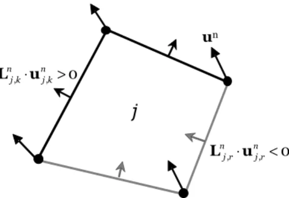
Finite Volume scheme relies on Lagrange-Remap approach, to stick to Vofire hypotheses [Després et al., 2010]. Lagrangian step is straightforward using nodal velocities obtained from Finite Elements and is not discussed. Balance equations within cell j of fluid unstructured mesh during Remap phase then write (see. Figure 2):
(
)
(
)
(
)
L u L u L u 1 , , , 1 1 1 , , , , , , , , 0 0 n n n n n f n j j j j j k j k j k k n n n n n n n n f n n n n f n n j j ij j j ij j k j k j k ij k j r j r j r ij r k N r N S ρ S ρ t ρ S ρ c S ρ c t ρ c t ρ c + + + + + − ∈ ∈ − + ∆ ⋅ = − + ∆ ⋅ + ∆ ⋅ =∑
∑
∑
ɶ ɶ ɶ ɶ (4)In (4), {N+} designates outgoing faces group for current cell (L u
, , 0 n n
j k⋅ j k> ), whereas {N-}
designates incoming faces group (L , u, 0 n n
j r⋅ j r< ).
Figure 2: Typical cell of an unstructured mesh
Equation (4) requires reconstructed quantities , f n j k
ρ and n,
i j k
c on outgoing faces to build fluxes for total fluid mass and fluid mass fractions. Defining a reconstruction strategy to control dissipation for mass fraction of gases is the main issue for next paragraph.
3. Extended Vofire algorithm to control dissipation for liquid-gas fast transient flows As evoked in § 2, controlling numerical dissipation of gas mass fraction is mandatory to perform accurate simulations involving liquid-gas interfaces without any reconstruction needing specific external variables. An illustration of this situation is given in next paragraph, whereas the following provide a description of an anti-dissipative strategy based on Vofire scheme with improvements imposed by physics considered in present paper.
3.1 Basic illustration of numerical dissipation
Figure 3 presents a simple 2D-plane simulation of an underwater explosion. A 20 bars bubble is immersed in liquid with free surface. Fluid is enclosed in a 1 m wide rigid square box. No anti-dissipation is used, i. e. reconstructed quantities are simply upwind quantities.
un
j
L , u , 0 n n j r⋅ j r< L , u , 0 n n j k⋅ j k>(a) Initial void fraction field (b) Void fraction field after 10 ms Figure 3: 2D-plane underwater explosion without anti-dissipation
Artificial mixing zone of gas and liquid largely spreads, making interface location very inaccurate.
3.2 Anti-dissipative principle
The main concept is presented using the simple case of monodimensional advection of a step function h in a constant velocity field u [Després et Lagoutière, 2001]. The problem, after Finite Volume spatial discretization with cell size ∆x, is described by Figure 4.
Figure 4: Monodimensional step function advection in constant velocity field
At one given time step within discrete time scale, with time step length ∆t, function front is located in cell j. The point is then to choose discrete value hj+1/2 for function h on cell boundary [j+1/2]
to build flux ∆ +
∆
u j1/2
t h
x involved in balance of function h in cell j between current time step and next
one.
This situation classically exhibits two limit cases, as shown on Figure 5:
Flux is zero as soon as hj is non-zero: discrete function propagates before its analytical front reaches boundary [j+1/2], yielding numerical dissipation. (a) Upwind: hj+1/2=h j j-1/2 j+1/2 j j-1 Continuous Discrete 1 1 u j-1/2 j+1/2 j+1 j j-1 Continuous values of h function Discrete values of h function
Flux is always zero. Numerical dissipation is blocked. Discrete solution is wrong when theoretical front propagates beyond boundary [j+1/2], since no transport occurs between cells j and j+1, yielding unstable growth of h in cell j.
(b) Downwind: hj+1/2=hj+1
Figure 5: Limit cases for choice of boundary value
These limit cases introduce base concept and numerical method from Desprès & Lagoutière: provide a mostly downwind advection scheme to control dissipation, associated to constraints preserving stability when a step propagates through cell boundaries (Downwind Scheme with
Constraints).
For present system, constraints express as follows:
Flux consistency: mj+1/2=min
(
h hj, j+1)
≤hj+1/2≤max(
h hj, j+1)
=Mj+1/2 (5-a)Advection stability: − =
(
−)
≤ ≤(
−)
= − * 1/2 min 1, max 1, 1/2 j j j j j j j m h h h h h M (5-b) with *= +u(
− − +)
1/2 1/2 j j j ∆t h h h h ∆xUsing inequation (5-a) on flux hj-1/2, a sufficient condition for stability is obtained:
(
)
(
)
− − + − + − ≤ + − + − ≤ u u 1/2 1/2 1/2 1/2 1/2 1/2 j j j j j j j j ∆t m h m h ∆x ∆t h M h M ∆x (6)This yields trust intervals for le hj+1/2:
(
)
(
)
+ + + − − + − − ≤ ≤ ∆ ∆ + − ≤ ≤ + − ∆ ∆ u u 1/2 1/2 1/2 1/2 1/2 1/2 1/2 1/2 j j j j j j j j j j m h M x x M M h h m m h t t (7)Intersection of these intervals is non-empty since upwind is always stable. Anti-dissipation is then achieved by choosing hj+1/2 closest to downwind within this intersection. Schemes can be derived for
multidimensional simulations on structured grid using Direction Splitting technique
3.2 Vofire algorithm for liquid-gas flow on unstructured grid
Three-component material from § 2.2 is now considered. Anti-dissipation is applied to capture interface between liquid and gas components, which means that variable c appearing in following formulae is in fact the sum of mass fraction of both gases. With this sum known on cell boundaries, transported mass fractions for each gas are deduced using upwind concentrations. Mass conservation Finite Volume equations during Remap phase thus write:
(
)
(
)
(
)
L u L u L u 1 , , , 1 1 1 , , , , , , , , 0 0 n n n n n f n j j j j j k j k j k k n n n n n n n n f n n n n f n n j j j j j j j k j k j k j k j r j r j r j r k N r N S ρ S ρ t ρ S ρ c S ρ c t ρ c t ρ c + + + + + − ∈ ∈ − + ∆ ⋅ = − + ∆ ⋅ + ∆ ⋅ =∑
∑
∑
ɶ ɶ ɶ ɶ (8)Let us also notice that in most simulations, gases do not mix, c then being mass concentration of either one gas or the other.
In original Vofire scheme, total mass conservation is treated independently from advection of component mass fractions, using a reconstructed total density ,
f n j k
ρ obtained from a second order finite volume scheme, so that total fluid mass transport equation can be solved and total fluid density in cell j is known at time step n+1.
j-1/2 j+1/2 j+1 j j-1 Discrete Continuous
To simplify next formulae, additional following notations are introduced:
(
)
(
)
(
)
(
)
L u L u L u L u , , , , , , , , , , , , , , ; ; n n f n n n f n j k j k j k j r j r j r j k j r n n f n n n f n j k j k j k j r j r j r k N r N ρ ρ p p L L L ρ L ρ + − + − + − ∈ ∈ ⋅ ⋅ = = =∑
⋅ =∑
⋅ (9) Transverse reconstructionFirst, transverse reconstruction provides slight anti-dissipation accounting for velocity field not aligning with mesh directions (see [Després at al., 2010] for detailed description of the phenomenon). Reconstructed concentration expresses as:
(
)
, , , , , 0,1 R n n n
j k j j k k j j k
c = +c λ c −c ∀ ∈k N λ+ ∈ (10)
, coefficients are chosen to minimize a functional J, measuring difference between
reconstructed mass fractions and downwind mass fractions for corresponding faces, with total outgoing mass kept constant compared to upwind case, yielding:
+ ∈ =
∑
, , − R j k j k k k N J p c c (11)(
)
+ ∈ − =∑
j k, k j j k, 0 k N p c c λ (12)Computation algorithm for coefficients , and complete geometric interpretation of transverse
reconstruction are detailed in [Després et a., 2010].
Longitudinal reconstruction
This step achieves most of anti-dissipative work. Main idea for Vofire scheme is to rewrite conservation of gas mass fraction equation into a convex sum of pseudo-monodimensional problems, each involving one incoming face and one outgoing face of current cell. To this extend, gas mass fraction on face k of cell j is decomposed as follows:
(
)
, , , , , , ; , , 0,1 n R n R j k j k j r j k r k j k j k r r N c c p µ c c µ − ∈ = +∑
− ∈ (13) n kc designates downwind value for outgoing face k (i.e. value in neighbor cell). If µj k r, , equals to 1
for all incoming faces r, value n k
c is obtained for , n j k
c , whereas if µj k r, , equals to 0 for all incoming faces,
value , R j k
c is obtained, i.e. upwind value after transverse reconstruction. Injecting decomposition (13) into balance (8) yields:
(
1 1 1)
(
)
, , , , , , , , , , , , , 1 1 1 , , , 0 n n n n n n R n R j k j r j j j j j j j k j r j k j r j k r k j k k N r N k N r N r N n j r j k j r r N k N n n n n n n j k j r j j j j j j k N r N p p S ρ c S ρ c t L p p c p µ c c t L p p c p p S ρ c S ρ c + − + − − − + + − + + + + ∈ ∈ ∈ ∈ ∈ − ∈ ∈ + + + ∈ ∈ − + ∆ + − +∆ = ⇔ − + ∆∑
∑
∑
∑
∑
∑
∑
ɶ ɶ ɶ ɶ(
)
{
, , , , , ,}
0 R n R n j k j k r j r k j k j r tL c+ +µ p c −c + ∆tL c− = (14)Sum is convex since
+ − ∈ ∈ =
∑
, , , 1 j k j r k N r N p p .Consistency condition for flux of mass fraction c is:
, min , , max , , n n n n n j k j k j k j k j k
m = c c ≤c ≤ c c =M (15)
Stability for mass fraction advection is given by:
( )
1( )
, ,
min n,min n n max n,max n
j j r N j r j j r N j r j m c − c c+ c − c M ∈ ∈ = ≤ ≤ = (16)
Thanks to convexity of sum (14), sufficient condition is obtained by imposing stability for each term:
1 , min , , max , , , n n n n n j r j j r j j j r j r m = c c ≤c + ≤ c c =M (17) Inequalities (17) provide trust intervals for coefficient µj k r, , associated to each incoming face,
using
m
j r,≤
c
nj r,≤
M
j r, (flux consistency for face r): Ifc
Rj k,>
c
nk:(
)
(
)
, 1 1 , , 1 1 , , , , , 1 n n n R 1 n n n R j r n n j j j j k j r n n j j j j k j j j j j k r R n R n j k k j k k m tL S ρ c tL c M tL S ρ c tL c S ρ S ρ µ tL c c tL c c − + − + + + + + + + − ∆ − − ∆ − ∆ − − ∆ ≤ ≤ ∆ − ∆ − ɶ ɶ ɶ ɶ (18-a) Ifc
Rj k,<
c
kn:(
)
(
)
, 1 1 , , 1 1 , , , , , 1 n n n R 1 n n n R j r n n j j j j k j r n n j j j j k j j j j j k r R n R n j k k j k k M tL S ρ c tL c m tL S ρ c tL c S ρ S ρ µ tL c c tL c c − + − + + + + + + + − ∆ − − ∆ − ∆ − − ∆ ≤ ≤ ∆ − ∆ − ɶ ɶ ɶ ɶ (18-b)µj k r, , is chosen closest to one in above intervals and final value for , n j k
c with anti-dissipation is obtained taking inequality (15) into account.
2.3 Extension to handle large density ratio between components
Original Vofire scheme is independent from equations of state used for components, but in the case of large density ratio, it presents numerical problems that require fixing [Faucher and Kokh, 2011].
1. Computing total density on outgoing faces independently from reconstructed mass fractions makes it impossible to completely empty a cell initially full of liquid by injecting pressured gas in it: total density for outgoing flux, which should remain equal to liquid density until all liquid has been chased, drops because of global reconstruction and too few liquid is pushed out of the cell at each time step, causing instability in the scheme. This can also be seen as the incapability of any second order scheme to reconstruct a sharp density step with several orders of magnitude between lowest and highest value.
2. Numerical dissipation is actually removed from simulation results, but artifacts appear on the interface when Vofire scheme is used on structured mesh (see Figure 6 for a basic illustration from example introduced in § 3.1), leading again to numerical instability.
(a) Initial void fraction field (b) Void fraction field after 10 ms
with original Vofire algorithm Figure 6: Artifacts on liquid-gas interface with Vofire scheme of structured grid
To fix problem 1, it is necessary to link mass fraction estimation and total density reconstruction. This is done by computing densities per component, evaluated upwind using component volume fractions, and a partition of an arbitrary volume of fluid considered on an outgoing face, into a liquid fraction and gas fraction:
(
)
, , 1 1 n n n n j j gas gas j k j n j n n n n j j liq liq j k j n j c ρ ρ ρ α c ρ ρ ρ α = = − = = − (19) = gas+ liq V V V (20)with V an arbitrary volume considered on current outgoing face This yields:
(
,)
, , , , , , 1 n n gas liq j k j k n n n nf n gas liq gas liq j k j k j k j k j k c m c m m m m ρ ρ ρ ρ ρ − = + = + ɶ (21)
with m the mass of fluid contained in volume V
New total density then writes:
(
)
, , , , , , , 1 n n gas liq j k j k f n j k n gasn n liqn j k j k j k j k c c = − + ɶ ρ ρ ρ ρ ρ (22)To compute total mass flux, an iterative procedure should be used, because of f n, j k ɶ ρ depending on , n j k c and computation of n, j k
c through Vofire scheme involving total density on outgoing faces. Practically, one iteration is enough to overcome problem 1:
, , , , Vofire Vofire f n n f n n j k j k j k j k ρ →c →ρɶ →cɶ , f n j k ρɶ and , n j k
cɶ are used to compute total mass flux and per component mass fluxes on outgoing faces.
Problem 2 is caused by spurious interaction between pseudo-monodimensional flows within a cell, some of which being non-physical, like those written between two orthogonal faces. This
interaction does not occur with direction splitting, producing correct results. Proposed solution is then to provide a geometric correction to Vofire scheme, modifying decomposition (13) into:
(
)
, , , , , , ; , , 0,1 n R n R j k j k j r j k r k j k j k r r N c c p µ c c µ − ∈ = +∑
ɶ − ∈ (23) with pɶj k r, , =βj k r, ,pj r, et − ∈ =∑
ɶj r, 1 r N p Then:(
)
, , , , , , , , ; , , 0,1 n R n R j k j k j k r j r j k r k j k j k r r N c c β p µ c c µ − ∈ = +∑
− ∈ (24)This introduces a minor change into (14), which does not affect computation procedure for coefficients µj k r, , :
(
)
{
1 1 1}
, , , , , , , , , , , 0 n n n n n n R n R n j k j r j j j j j j j k j k r j k r j r k j k j r k N r N p p S ρ c S ρ c tL c β µ p c c tL c + − + + + + − ∈ ∈ − + ∆ + − + ∆ =∑
ɶ ɶ (25)New trust intervals are: If
c
Rj k,>
c
kn :(
)
(
)
, 1 1 , , 1 1 , , , , , , , , , 1 n n n R 1 n n n R j r n n j j j j k j r n n j j j j k j j j j j k r R n R n j k r j k k j k r j k k m tL S ρ c tL c M tL S ρ c tL c S ρ S ρ µ β tL c c β tL c c − + − + + + + + + + − ∆ − − ∆ − ∆ − − ∆ ≤ ≤ ∆ − ∆ − ɶ ɶ ɶ ɶ (26-a) Ifc
Rj k,<
c
kn :(
)
(
)
, 1 1 , , 1 1 , , , , , , , , , 1 n n n R 1 n n n R j r n n j j j j k j r n n j j j j k j j j j j k r R n R n j k r j k k j k r j k k M tL S ρ c tL c m tL S ρ c tL c S ρ S ρ µ β tL c c β tL c c − + − + + + + + + + − ∆ − − ∆ − ∆ − − ∆ ≤ ≤ ∆ − ∆ − ɶ ɶ ɶ ɶ (26-b)The aim of replacing weights pj r, by weights pɶj k r, , for outgoing face k is to remove from the sum
all incoming faces with an angle higher than 90° with respect to face k. Physically, it means that it is not suitable to consider a fictitious monodimensional flow between two faces with opposite
orientation. For the special case of a structured grid, faces are associated 2 by 2 as with direction splitting. ɶj k r, , p thus writes:
(
n n)
, , , max , ,,0 , j k r j k j k j r j r pɶ =γ ⋅− p (29) with j k, max(
nj k, nj q, ,0)
j q, q N γ p − ∈ =∑
⋅− and(
)
(
)
n n n n , , , , , , , max ,0 max ,0 j k j r j k r j k j q j q q N β p − ∈ ⋅− = ⋅−∑
, j kγ equal to zero means that no incoming face remains for outgoing face k. Anti-dissipation is then useless and , , n R j k j k c =c . , j k
γ going down to zero implies coefficientsβj k r, , growing to infinity. Stability of associated
monodimensional problems given by (26-a&b) tends to impose upwind solution, which converges continuously towards solution with γj k, equal to zero.
Figure 7 shows results with corrected Vofire algorithm on previous test case compared to original Vofire solution, demonstrating artifacts disappearance.
(a) Initial void fraction field (b) Void fraction field after 10 ms
with original Vofire algorithm
(c) Void fraction field after 10 ms with corrected Vofire algorithm Figure 7: Effect of corrected Vofire scheme on interface artifacts
4. Elementary validations
All following tests are performed using EUROPLEXUS Software1,2 (abbreviated EPX in the
following paragraphs), a fast transient dynamics program co-owned by French Commissariat à
l’Energie Atomique et aux Energies Alternatives (CEA) and European Commission.
As far as numerical performances are concerned, EPX relies on a distributed memory parallel solver with automatic domain decomposition [Faucher, 2011]. Vofire reconstruction of mass fractions on cell boundaries is completely local to a cell and its immediate neighbors, so that it naturally benefits from parallel acceleration, which is more difficult to obtain with an external representation of
interfaces.
4.1 Liquid-gas shock tube
First elementary test is a basic liquid-gas shock tube with high pressure ratio, designed to demonstrate program’s capability to capture strong contact discontinuity between fluid components, even with a relatively coarse mesh. Setup is given by Figure 8.
Figure 8: Liquid-gas shock tube
Figure 9 presents results in terms of both pressure and density fields along the tube, after 0.09 ms, 0.18 ms and 0.27 milliseconds. Shock wave propagates in liquid whereas rarefaction wave propagates in the opposite direction in gas. Density step should remain sharp if no spurious mixing occurs between components.
On Figure 9, reference solution is obtained with time and space second order finite volume scheme with very fine mesh (50 000 cells). Other solutions are obtained with 1 000 cells along the tube and with/without Vofire anti-dissipative scheme.
(a) Pressure field along the tube
1http://europlexus.jrc.ec.europa.eu/public/manual_html/index.html 2http://www.repdyn.fr 0 2 000 4 000 6 000 8 000 10 000 12 000 0,0 0,1 0,2 0,3 0,4 0,5 0,6 0,7 0,8 0,9 1,0 P re s s u re ( b a rs )
Abscissa along the tube (m)
Gas – 10 000 bars – 720 kg.m-3 Liquid – 1 bar – 1 000 kg.m-3
1 m Reference solution Solution with no anti-dissipation Vofire solution
(b) Density field along the tube Figure 9: Liquid-gas shock tube solutions
As expected, anti-dissipation does not modify pressure field, as well as density profiles for shock wave and rarefaction wave. On the contrary, growing artificial mixing zone appears with no anti-dissipation, whereas Vofire allows a very accurate location of liquid-gas interface.
4.2 Sloshing in a decelerated tank
Second test illustrates the need for anti-dissipative techniques to correctly simulate the force applied by internal fluid to surrounding structure in the case of large fluid motion with severe external loading. Considered situation is a parallelepipedic rigid tank partially filled with liquid and submitted to a global deceleration close to those encountered during a car crash. Experimental data in this configuration is available from [Nakano and Iwamoto, 1988].
Model is bidimensional and described on Figure 10. Pressure in liquid is initialized with hydrostatic pressure.
(a) Setup (b) Deceleration force field along time
Figure 10: Model for decelerated tank simulation
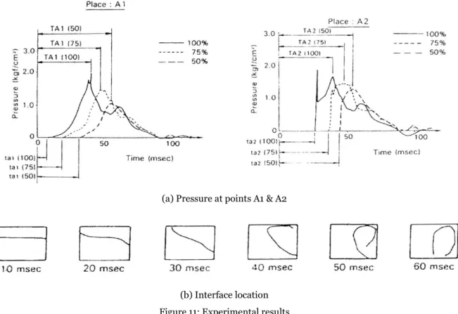
Figure 11 presents experimental results extracted from original paper in terms of pressure time history for points A1 and A2 located on Figure 10 and interface location measured with fast camera (tank is transparent). Several tests were performed with different filling levels. Simulated test among those appearing on Figure 11 is named “75 %”. Pressure unit is kgf/cm2, i.e. 105 Pa, i.e. 1 bar. Reference
pressure is atmospheric pressure.
0 200 400 600 800 1 000 1 200 1 400 0,0 0,1 0,2 0,3 0,4 0,5 0,6 0,7 0,8 0,9 1,0 D e n s it y ( kg /m 3)
Abscissa along the tube (m)
0 50 100 150 200 250 300 350 400 0,00 0,02 0,04 0,06 0,08 0,10 0,12 0,14 0,16 0,18 0,20 H o ri z o n ta l d e c e la ra ti o n ( m /s 2) Time (s) Liquid – hydrostatic pressure
Gas – 1 bar
Global deceleration force
460 mm A1 A2 3 0 0 m m
(a) Pressure at points A1 & A2
(b) Interface location Figure 11: Experimental results
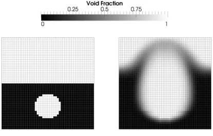
Figure 12 presents simulation results, again with and without Vofire anti-dissipative scheme. Regular mesh is used with 1 mm cell size. Pressure is plotted taking atmospheric pressure as reference (i.e 1 bar) for comparison with experiments. To locate the interface, density field is drawn with specific color bar, so that gas appears white, liquid appears gray and mid-value between reference densities of gas and liquid appears black.
(a) Pressure at point A1
-0,4 -0,2 0 0,2 0,4 0,6 0,8 1 1,2 1,4 1,6 1,8 0 0,02 0,04 0,06 0,08 0,1 0,12 P re s s u re ( b a rs ) Time (s) Vofire solution Solution with no anti-dissipation
(b) Pressure at point A2
20 ms 30 ms 40 ms 50 ms
60 ms 70 ms 90 ms 120 ms
(c) Interface location without anti-dissipation
20 ms 30 ms 40 ms 50 ms
60 ms 70 ms 90 ms 120 ms
(d) Interface location with Vofire scheme Figure 12: Sloshing simulation results
-0,2 0 0,2 0,4 0,6 0,8 1 1,2 1,4 1,6 0 0,02 0,04 0,06 0,08 0,1 0,12 P re s s u re ( b a rs ) Time (s)
Despite a ~10 ms time shift, simulated pressure curves show good agreement with experimental reference and little improvement is provided by Vofire algorithm. On the contrary, anti-dissipation is compulsory to maintain gas cavity shape after complete fuel reversal, as shown by experimental results. Even with a relatively fine mesh, dissipation modify mass flow along walls, resulting in a non-physical jet, composed of mixed liquid and gas, arriving too early at bottom right corner of the box at time 70 ms and then destroying cavity envelop.
5. Industrial application: simulation of MARA 10 experiment
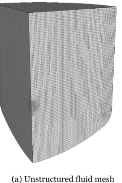
Physical set-up is described in § 2.1. Corresponding numerical model is presented on Figure 13.
(a) Unstructured fluid mesh (b) Structural mesh
Figure 13: MARA 10 numerical model
Material behavior law for structures is elasto-plastic steel, except for massive part of Core
Structure Support, made of elasto-plastic copper-aluminium alloy AU4G. Isotropic Von Mises criterion is used in both cases for plastic hardening. Elastic limits are given on Table 1 and structural shell thicknesses on Table 2. Table 3 presents values for fluid equations of state parameters. Geometry is axisymmetrical and a 3D simulation is carried out, 1/4 of the model being meshed with suitable symmetry conditions.
Elastic limit (MPa)
Vessel lateral surface 336
Vessel corner 600
Vessel bottom surface 450
Above Core Structures 336
Diagrid 312
Radial Shield 378
Thin Core Support Structure 274
Massive Core Support
Structure 220
Roof 245
Thickness (mm) Vessel lateral and bottom
surfaces
1.25
Vessel corner 1
Above Core Structures 1
Diagrid 0.9
Radial Shield 0.5
Thin Core Support Structure 1.3
Roof 10
Table 2: Structural shell thicknesses
Bubble gas Blanket gas Water
Parameter Polytropic power γ coefficient Sound speed
Value 1.24 1.4 1 500 m.s-1
Table 3 : Parameters for fluid equations of state
Fluid mesh is conformant with lagrangian structural mesh along roof and vessel envelop, whereas internal structures are immersed into fluid mesh with topological disconnection (see § 2.3). Vofire scheme is used to control dissipation of component mass fractions, between explosive bubble and water on the one hand, and between water and gas blanket on the other hand.
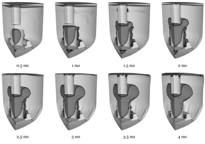
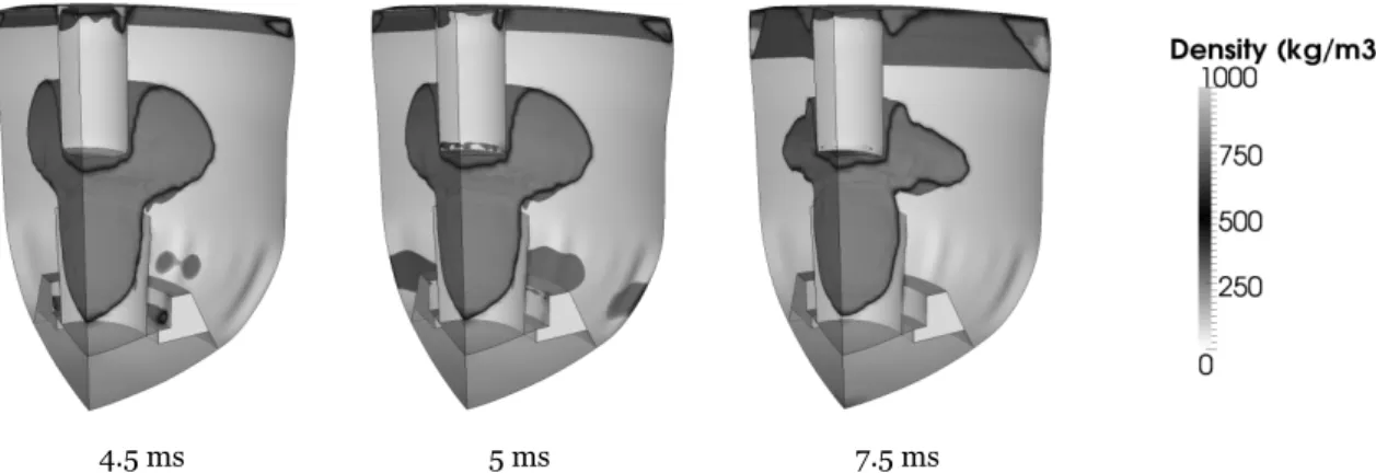
Figure 14 presents results in terms of structural deformed shape and density field in fluid. Same colorbar is used as in § 4.2, to locate interfaces between liquid and gases.
0.5 ms 1 ms 1.5 ms 2 ms
4.5 ms 5 ms 7.5 ms
Figure 14: Deformed shape of structures and density field in fluid
Interfaces are sharply captured, especially for water impact on the roof at time 2.5 ms and explosive gas bubble expanding through the opening between Above Core Structures and Radial Shield. Other bubbles appear in liquid domain behind Radial Shield, above Core Support Structure and under Diagrid. These come from a simplified cavitation model in liquid to handle situations where pressure tends to go down to negative values. Their potential interaction with explosive gas bubble is handled in Vofire scheme by correcting total density computation from reconstructed component mass fractions [Faucher and Kokh, 2011].
From structural point of view, a bulge appears at junction between roof and vessel, due to air blanket compression, which is a characteristic phenomenon for this series of tests. Radial buckling instability occurs in lower part of the vessel, consecutive to vessel bottom lowering, which shows interest for such 3D simulations even with axisymmetrical geometry.
Table 4 provides basic comparisons between simulation and experimental results.
Experiment Simulation
Maximum Final Maximum Final
Vessel bottom vertical
displacement (cm)
3.8 2.7 2.6 2.4
Vessel bulge radial displacement (cm)
0.10 0.09 0.11 0.10
Vessel bulge distance to the roof (cm)
6.3 7.2
Table 4: Comparisons between experiments and simulation
Simulation slightly overestimates structural displacements near the bulge on the one hand and underestimates vessel bottom vertical displacement on the other hand. This is mainly due to large structural strain rates with sharp water impacts, which is not taken into account in material behavior for this illustrative calculation and has less influence with smoother impacts when no anti-dissipation is used. Consequently, material behavior is too soft at vessel top, whereas vessel bottom is protected by excessive plastic strain dissipation within Diagrid and Core Support Structure.
Agreement between experimental data and calculation is yet satisfactory.
5. Conclusion
An algorithm is proposed to simulate fast transient liquid-gas flows in interaction with structures without explicitly describing interfaces between components, which provides robustness and
numerical efficiency necessary to handle generic industrial simulations with large structural displacements.
Accuracy in interface location is achieved by improved Vofire scheme, based on downwind mass fraction reconstruction to prevent numerical dissipation, with theoretically mastered constraints to maintain stability of advection scheme. Difficulties with original Vofire scheme specific to high density ratio between liquid and gas are identified and solved. Method is validated on elementary tests and its industrial potential is illustrated through the simulation of MARA 10 experiment.
Further work will be dedicated to extending the scheme to any number of components, only one interface between liquid and equivalent gas being currently considered, to generalize approach for other equations of state and to analyze potentialities of high order anti-dissipative schemes.
References
Acker D., Benuzzi A., Yerkess A., Louvet J., 1981, MARA 01/02 – experimental validation of the SEURBNUK and SIRIUS containment codes, in Proceedings of the Sixth International Conference on Structural Mechanics in Reactor Technology, Paper E 3/6, Paris, France.
Allaire G. Clerc S., Kokh S., 2002, A five-equation model for the simulation of interfaces between compressible fluids, J. Comput. Phys. 181(2): 577-616.
Després B., Lagoutière F., 2001, Contact discontinuity capturing schemes for linear advection and compressible gas dynamics, J. Sci. Comp. 16: 479-524.
Després B., Lagoutière F., 2007, Numerical resolution of a two-components compressible fluid model with interfaces, Prog. Comp. Fluid Dyn. 7(6): 295-310.
Després B., Lagoutière F., Labourasse E., Marmajou I., 2010, An Anti-dissipative Transport Scheme on Unstructured Meshes for Multicomponent Flows, Int. J. Finite Volumes 7: 30-65.
Casadei F., 2008, Fast Transient Fluid-Structure Interaction with Failure and Fragmentation, 8th World Congress on Computational Mechanics, June 30 – July 5, Venice, Italy.
Faucher V., 2011, Advanced parallel computing for explosive fluid-structure interaction, COMPDYN 2011, May 26-28, Corfu, Greece.
Fiche C., Louvet J., Smith B. L., Zucchini A., 1985, Theoretical experimental study of flexible roof effects in an HCDA’s simulation, in Proceedings of the Eighth International Conference on Structural Integrity in Reactor Technology, Paper E 4/5, Brussels, Belgium.
Glimm et al., 1998 – Three-dimensional Front Tracking, SIAM J. Sci. Comp. 19: 703-727. Lafaurie B., Nardone C., Scardovelli R., Zaleski S., Zanetti G.,1994, Modelling merging and fragmentation in multiphase flows with SURFER, J. Comput. Phys. 113: 134-147.
Louvet J., Hamon P., Smith B. L., Zucchini A., 1987, MARA 10: an integral model experiment in support of LMFBR containment analysis, in Proceedings of the Ninth International Conference on Structural Mechanics in Reactor Integrity, vol. E, Lausanne, Switzerland.
Kokh S., Lagoutière F., 2010, An anti-diffusive numerical scheme for the simulation of interfaces between compressible fluids by means of a five equation model, J. Comput. Phys. 229: 2773-2809. Mosso S., Cleancy S., 1995, A geometrical derived priority system for Young’s interface reconstruction, LA-CP-95-0081, LANL report.
Nakano M., Iwamoto T., 1988, Analysis of the Behavior of Liquid in a Fuel Tank, SAE Technical Paper Series, Passenger Car Meeting and Exposition, October 31 – November 3, Dearborn, Michigan, USA. Rider W. J., Kothe D. B., 1995, Stretching and tearing interface tracking methods, AIAA Paper, 95: 1-11.
Robbe M. F., Lepareux M., Treille E., Cariou Y., 2003, Numerical simulation of a Hypothetical Core Disruptive Accident in a small-scale model of a nuclear reactor, Nuclear Engrg. and Design 223: 159-196.
Scardovelli R., Zaleski S., 1999, Direct numerical simulation of free-surface and interfacial flow, Annual Review Of Fluid Mechanics 31: 567-603.
Smith B. L., Yerkess A., Adamson J., 1983, Status of coupled fluid-structure dynamics code
SEURBNUK, in Proceedings of Seventh International Conference on Structural Mechanics in Reactor Technology, Paper B 9/1, Chicago, USA.
Sussman M., Smereka P., Osher S., 1994, A Level Set Approach for Computing Solutions to Incompressible Two-Phase Flow, J. Comput. Phys. 114(1): 146-159.
Unverdi S., Tryggvason, 1992, A front-tracking method for viscous incompressible multi-fluid flows, J. Comput. Phys. 100: 25-37.