Decision Under Normative Uncertainty

HAL Id: halshs-01877769

https://halshs.archives-ouvertes.fr/halshs-01877769

Preprint submitted on 20 Sep 2018

HAL is a multi-disciplinary open access archive for the deposit and dissemination of sci-entific research documents, whether they are pub-lished or not. The documents may come from teaching and research institutions in France or abroad, or from public or private research centers.

L’archive ouverte pluridisciplinaire HAL, est destinée au dépôt et à la diffusion de documents scientifiques de niveau recherche, publiés ou non, émanant des établissements d’enseignement et de recherche français ou étrangers, des laboratoires publics ou privés.

Decision Under Normative Uncertainty

Franz Dietrich, Brian Jabarian

To cite this version:

WORKING PAPER N° 2018 – 46

Decision Under Normative Uncertainty

Franz Dietrich

Brian Jabarian

JEL Codes:

Keywords :

P

-

S

E

48, BD JOURDAN – E.N.S. – 75014 PARIS

TÉL. : 33(0) 1 80 52 16 00=

www.pse.ens.fr

CENTRE NATIONAL DE LA RECHERCHE SCIENTIFIQUE – ECOLE DES HAUTES ETUDES EN SCIENCES SOCIALES

ÉCOLE DES PONTS PARISTECH – ECOLE NORMALE SUPÉRIEURE

Decision Under Normative Uncertainty

September 20181

Franz Dietrich

Paris School of Economics & CNRS

Brian Jabarian

U. Paris 1 & Paris School of Economics

Abstract

How should we evaluate options when we are uncertain about the correct standard of evaluation, for instance due to con‡icting normative intuitions? Such ‘normative’ uncertainty di¤ers from ordinary ‘empirical’uncertainty about an unknown state, and raises new challenges for decision theory and ethics. The most widely discussed pro-posal is to form the expected value of options, relative to correctness probabilities of competing valuations. But this meta-theory overrules our beliefs about the correct risk-attitude: it for instance fails to be risk-averse when we are certain that the correct (…rst-order) valuation is risk-averse. We propose an ‘impartial’meta-theory, which re-spects risk-attitudinal beliefs. We show how one can address empirical and normative uncertainty within a uni…ed formal framework, and rigorously de…ne risk attitudes of theories. Against a common impression, the classical expected-value theory is not risk-neutral, but of hybrid risk attitude: it is neutral to normative risk, not to empirical risk. We show how to de…ne a fully risk-neutral meta-theory, and a meta-theory that is neutral to empirical risk, not to normative risk. We compare the various meta-theories based on their formal properties, and conditionally defend the impartial meta-theory.

1

Normative versus empirical uncertainty

Suppose we must evaluate some choice options. The criterion could take several forms, for instance personal well-being, ‘utility’in a suitable sense2, moral value, social welfare,

1_{We thank various colleagues for stimulating exchanges and in some cases extensive comments. We}

wish to mention (in alphabetic order) Ron Aboodi, Roland Bénabou, David Black, Richard Bradley, Ryan Doody, David Enoch, Marc Fleurbaey, Hilary Greaves, Alan Hajek, Sergiu Hart, Seth Lazar, François Maniquet, Ittay Nissan-Rozen, Katie Steele, Jean-Marc Tallon, Christian Tarsney, Aron Vallinder, Brian Weatherson, and Stéphane Zuber. We also received useful feedback when the paper was presented, such as in the Decisions, Ethics and Uncertainty Reading Group at Hebrew University of Jerusalem (April 2018), the Ethics and Uncertainty Workshop at Hebrew University of Jerusalem (June 2018), the Norms and Normativity Congress at ENS Lyon (June 2018), and the yearly Kick-O¤ Workshop of Paris School of Economics (September 2018). Franz Dietrich acknowledges support by the French National Research Agency through the grant “Coping With Heterogeneous Opinions” and through an EUR grant. Brian Jabarian acknowledges support through a Global Excellence Gulbenkian Scholarship.

2_{The ‘utility’in question must be something about which there is a fact and hence a possible}

uncer-tainty, such as rational desirability, personal interest, or true desire level (all of which are controversial concepts).

legal value, or artistic value. In this evaluation, one can face two fundamentally di¤erent types of uncertainty. Decision theory has so far focused on empirical uncertainty: uncertainty about empirical facts, states, or consequences of options. A doctor may be uncertain whether a particular treatment cures the patient. Philosophers have recently turned to so-called normative uncertainty: uncertainty about the correct standard of evaluation itself (e.g., Oddie 1994, Lockhart 2000, Jackson and Smith 2006, MacAskill 2014, Bradley and Drechsler 2014, Ross 2006, Sepielli 2006, 2009, Weatherson 2014, Grieves and Ord 2017, Lazar 2017, MacAskill and Ord forth.).3 Even if the treatment is certain to cure the disease and known also in all its other empirical features –so that no empirical uncertainty whatsoever exists –the doctor can be uncertain about the moral value of the treatment, perhaps by wondering about the moral trade-o¤ between the recovery and the (fully known) side e¤ects of the treatment, or by hesitating between utilitarian and deontological evaluations.4 Normative uncertainty can be more pressing and harder to resolve than empirical uncertainty – which makes it more surprising that formal decision theory so far neglects normative uncertainty. But is normative uncertainty truly distinct and meaningful?

Why ordinary choice theory does not yet capture normative uncertainty. Before proceeding, we brie‡y address two misunderstandings or prejudices one can have about the notion of normative uncertainty. Firstly, might normative uncertainty be reducible to empirical uncertainty after all, so that decision theorists could continue working with a single type of uncertainty? No doubt, many would suspect this. But a reduction fails, for conceptual and formal reasons. Conceptually, a reduction con‡ates fundamentally distinct phenomena. Uncertainty about value is not uncertainty about empirical features or consequences of options. Uncertainty whether a utilitarian or deontological valuation is correct is fundamentally evaluative uncertainty, compatible with full certainty about empirical features and consequences. Formally, can standard choice theory not already capture normative uncertainty, after suitably re-interpreting standard choice-theoretic models? It can not. By re-interpreting Savage’s nature states as empirical-normative states, or re-interpreting von-Neumann-Morgenstern’s lotteries as lotteries over empirical-normative outcomes, we change not just the interpretation, but also the formal game itself. Why? If nature states suddenly contain value informa-tion, then they anticipate the evaluation of consequences by encoding the utility of each consequence –something compatible with neither ordinary expected-utility theory nor even state-dependent expected-utility theory.5 Analogously, classical expected-utility theory in von-Neumann-Morgenstern’s lottery setting is inconsistent with building value information (‘utility information’) into outcomes, because classical utilities are free parameters, determined by preferences rather than pre-determined by information ‘in’ outcomes.

3

Harsanyi’s (1978) impartial observer can be interpreted as facing normative uncertainty.

4_{In general, the doctor may wonder (i) which properties of the treatment matter morally, and (ii)}

how they matter (Dietrich and List 2013, 2017).

5_{Choice theorists rarely allow utilities of consequences to depend on states, and where they do (i.e.,}

in state-dependent expected-utility theory ) they still take utilities to be up to the agent rather than written into states.

Is normative uncertainty meaningful? There can be uncertainty only where there are facts – but are there normative facts? Is there a ‘right’ standard of evaluation, an object of uncertainty? For the sake of argument, let ‘value’ be ‘moral value’ (but the issue is similar for other types of value). We cannot dig into ongoing meta-ethical debates here, but we hasten to stress that full-blown moral realism is not required to make sense of moral uncertainty. Moral uncertainty exists meaningfully under a range of meta-ethical positions. Moral facts could be subjective rather than objective: their existence could depend on attitudes of agents, be they ideal agents or even the decision-maker himself. Moral facts could be relative rather than universal, as claimed by cultural or social relativism. And moral facts could be understood in the sense of meta-ethical constructivisms. Error-theoretic positions should however be excluded, as they deny moral facts. It is debatable whether certain non-cognitivist (e.g., ex-pressivist) positions are compatible with moral uncertainty, through some non-literal interpretation of ‘moral uncertainty’ which needs no moral facts (Weatherson 2014, Sepielli 2017).

2

De…ning the problem and its expected-value solution

To set the stage in due precision, we now carefully de…ne the framework in a standard version, and the expected-value approach. Later we shall add empirical uncertainty to the framework.

The objects of evaluation. We consider a non-empty set A of objects of evalu-ation, called ‘options’. They could be policy measures, social arrangements, income distributions etc. So far we leave open whether options contain empirical risk.

The competing valuations. Options have uncertain value, for instance because of competing normative intuitions or theories. Following the expected-value approach, our notion of value is numerical, not just comparative (for a defence, see MacAskill and Ord forth.). We thus represent a possible standard of evaluation by a function v, called a (…rst-order) valuation or theory, assigning to each option a in A a value v(a) in R. For instance a utilitarian valuation de…nes v(a) as total happiness resulting from a. But not all functions from A to R are plausible valuations. Implausible valuations, like that in terms of resulting unhappiness, can be excluded from consideration. Let V be the set of valuations/theories considered, formally a …nite non-empty set of functions from A to R. V might contain just two valuations, a utilitarian and a Rawlsian one, or a deontological and an egalitarian one. Alternatively, V might consist of many valuations of similar type di¤ering only in one parameter: prioritarian valuations with di¤erent degrees of prioritarianism, or egalitarian valuations with di¤erent degrees of inequality-aversion, or valuations of intertemporal (individual or social) well-being with di¤erent discounting of future well-being, or valuations (of risky options) with di¤erent degrees of risk-aversion, etc. If V is such a parametric family of valuations, the normative uncertainty is an uncertainty about the correct parameter value: the correct amount of prioritarianism, inequality-aversion, discounting, risk-aversion, etc.

Correctness probabilities of valuations. _{Each valuation v in V has a …xed} cor-rectness probability P r(v) 0, whereP_v2VP r(v) = 1. Probabilities capture degrees of belief about value (other interpretations are possible). The possibility to quantify normative uncertainty through sharp probabilities is a standard assumption.

Meta-valuations. What is the overall value of options given the normative uncer-tainty? Any answer is a meta-valuation or meta-theory, formally another function as-signing to each option in A a value in R. To distinguish it from …rst-order valuations, it is generically denoted as an upper-case V . So V (a) represents a’s overall value. Many potential meta-valuations come to mind. For instance, an option a’s overall value might be its minimal value across all …rst-order theories of non-zero probability: V (a) = min_{v2V:P r(v)6=0}v(a).6

Convention. We shall often say ‘valuation’ or ‘theory’ simpliciter, dropping ‘…rst-order’or ‘meta-’, provided there is no ambiguity.

Expected value theory (‘_{EV ’). This meta-theory evaluates each option a 2 A by} its expected value:

EV (a) =X

v2V

P r(v)v(a):

Here, overall value is average …rst-order value, weighted by correctness probabilities. Measurability and comparability of value. The expected value theory is some-times criticized for relying on numerical measurements and cross-theory comparisons of value. Measurability makes it meaningful for an option x to have value 7 under a valuation v (v(x) = 7), or be twice as valuable as another option y (v(x) = 2v(y)), or exceed y’s value by 2 (v(x) v(z) = 2), etc. Comparability makes it meaningful for option x to be equally valuable under two valuations v and v0 (v(x) = v0(x)), or more valuable under v than option y is under v0 (v(x) > v0(y)), etc.

Setting this debate aside, we show that the expected value theory is problematic even if value is fully measurable and cross-theory comparable. We thus retain this classic assumption throughout the paper (although it could be partly relaxed7_{). Note}

that comparability across valuations seems less problematic if V consists of valuations of similar type (e.g., egalitarian valuations with di¤erent degrees of inequality-aversion), but more debatable if V contains radically di¤erent valuations such as consequentialist and deontological ones.

6

For convenience, we de…ne meta-theories as value functions, not (binary) value relations, thereby invoking levels of, not just comparisons in, overall value. Everything could be restated using purely relational meta-theories.

7

The expected value theory and its three alternatives introduced below do not need full measurability of value: value need only be measurable on an a¢ ne scale, so that valuations are only unique up to increasing a¢ ne transformation. Further, the expected value theory does not need full comparability of value across theories: unit comparability without level comparability su¢ ces. Our impartial meta-theory however needs value comparability. Comparability and measurability are addressed by Bossert and Weymark (2004), and in the context of normative uncertainty by, e.g., Ross (2006) and Spirelli (2009).

Value versus von-Neumann-Mogenstern (‘vNM’) utility. The value of an option under a valuation in V should normally not be interpreted as a vNM utility (or expected vNM utility if the option is risky). To see why, consider a hedonistic theory v in V. It evaluates riskless options by the amount of experienced pleasure generated by the option. For any t 0, consider the option at2 A of donating t coins to a charity. Let the

agent’s pleasure from donating be never saturated: the …rst donated coin gives as much pleasure as the second, the second as much pleasure as the third, etc. Then the value of donating t coins, v(at), is linear in t. But the vNM utility of atmay or not be linear in

t, depending on the risk attitude of the evaluative theory in question: the vNM utility of at is linear, concave or convex in t (and in v(at)), depending on whether we consider

risk-neutral, risk-averse or risk-prone hedonism, respectively.8 Simply replacing v by a vNM utility function (or expected -vNM-utility function if A also contains risky options) is inappropriate, as we would then incorrectly measure pleasure gains: for instance, the vNM utility function of risk-averse hedonism rises less from a1 to a2 than from a0

to a1 (by concavity), although the pleasure gain is the same both times. The vNM

approach is ill-suited for the measurement and inter-theory comparison of value. See Broome (1991), Weymark (1991) and Nissan-Rozen (2015) for various analyses of the controversial value-utility relationship.

3

Two problems of the expected value theory

This section raises two objections against expected value theory, and proposes some principles, interpretable either as general normative principles or as methodological principles for designing operational meta-theories. We draw on empirical uncertainty, besides normative uncertainty. The possibility that options carry empirical uncertainty – e.g., uncertainty about consequences – is often acknowledged and explicitly allowed in the literature (Weatherson 2014, Nissan-Rozen 2016, MacAskill and Ord forth.), although empirical uncertainty is usually not formalized (an exception is Bradley and Drechsler 2013). Our objections and principles will so far be stated informally, as we postpone the formalization of empirical uncertainty to Section 5.

3.1 Overruling beliefs about the correct risk attitude

Consider two options a and b in A. Think of them as containing no empirical risk: their features are fully known. Let there be just two competing valuations v and v0 in V, each of correctness probability 12. Table 1 shows how each option is evaluated by v

and v0, and by the expected value (meta-) theory.

We can make the example concrete. Ann, Bob, and Claire su¤er from a disease. Ann owns 2g of a medicine, which is just enough to cure her. Bob and Claire would each need just 1g of that medicine to be cured. The agent (e.g., a public health authority) can either not intervene, so that Ann is cured by her medicine while Bob and Claire

8

Risk-neutral, -averse, and -prone hedonism is an extension of hedonism to risky prospects which regards the value of a risky prospect as being equal, below, or above the expected amount of resulting hedonic pleasure, respectively. This can be stated formally if A contains risky options of the sort ‘donating so-and-so many coins with such-and-such probabilities’.

evaluation by option v v0 meta-theoryEV

a 2 2 2 =1₂2+1₂2 b 4 0 2 =1₂4+1₂0

Table 1: Same overall evaluation despite di¤erent levels of value risk

stay ill. This is option a. Or the agent con…scates Ann’s medicine and redistribute it among Bob and Claire, so that Bob and Claire get cured while Ann stays ill. This is option b. Curing someone contributes two units of well-being to that person. Let v be a utilitarian theory which evaluates options by total resulting well-being. So option a has value 2 (one person cured) while b has value 4 (two persons cured). Theory v0 is a deontological theory which also attaches importance to the respect of property. It evaluates options by total resulting well-being, minus 4 in case of property violation. So option a has value 2 (one person cured, property respected), while b has value 0 = 4 4 (two persons cured, property violated).

The options a and b have the same expected value of 2. But assigning same overall value to a and b is problematic, as b contains normative uncertainty while a does not. By giving b overall value 2, one is neutral to the normative risk in b. Such meta-theoretic risk-neutrality can overrule a unanimous risk attitude among …rst-order valuations. It can indeed happen that

some option c displays exactly the same risk as b in terms of resulting value, except that the source of risk is empirical rather than normative,

the …rst-order valuations v and v0 evaluate c identically, at a same risk premium, although the expected value (meta-) theory evaluates b at no risk premium. For example, assume both valuations v and v0are risk-averse: risky options –options which could result in di¤erent empirical worlds according to certain probabilities –are evaluated below the expected value of the resulting world. Let risky option c result in a ‘positive’ or a ‘negative’ world, each with probability 1₂. These worlds have value 4 and 0 respectively, according to both v and v0.9

Option c can be made concrete. Imagine a second medicine which can only cure Bob, for generic reasons say. With probability 1₂, that medicine has a terrible side e¤ect reducing Bob’s well-being by 4 units. Option c consists in giving Bob that medicine, without redistributing Ann’s medicine. c results

either in the ‘positive’world without side e¤ect, of value 4 under both valuations (two persons cured, no side e¤ect, property respected),

or in the ‘negative’world with side e¤ect, of value 0 = 4 4 under both valuations (two persons cured, one su¤ering side e¤ect, property respected).

Being risk-averse, v and v0 evaluate c below the expected resulting value of 2 =

1 24 +

1

20. We assume v(c) = v(c0) = 1, amounting to a risk premium of 2 1 = 1:

The options b and c both lead to the same value prospect : the prospect that the resulting value is 4 with probability 1₂ and 0 with probability 1₂. So b and c display the

9

So a hypothetical option which surely results in the ‘positive’world has value 4, while a hypothetical option which surely results in the ‘negative’world has value 0, under both theories.

same risk in terms of resulting value, although the source of risk is normative for b and empirical for c. Since this risky value prospect justi…es a risk premium of 1 according to v and v0 _{(given how v and v}0 _{evaluate c), one would have expected the meta-theory}

to adopt this unanimous risk aversion, even where the source of risk is normative. This suggests evaluating b at a risk premium –against the expected value theory.

In sum, the expected value theory can create the awkward situation of neutrality to normative risk paired with aversion to empirical risk. Such a hybrid risk attitude is at least question-begging, as one wonders what would justify neutrality to normative risk if one should certainly be averse to empirical risk.

More systematically speaking, the expected-value theory violates the following prin-ciple:

Risk-Attitudinal Unanimity Principle (stated informally): If there is certainty about the correct risk-attitude, i.e., all valuations in V of positive probability have same risk attitude, then the meta-theory adopts this risk attitude (even towards normative risk).

The following broader principle also covers cases of risk-attitudinal heterogeneity or uncertainty:

Risk-Attitudinal Impartiality Principle (stated informally):The meta-theoretic risk attitude re‡ects impartially the beliefs about the correct risk-attitude captured by the correctness probabilities of …rst-order theories.

This principle requires forming a compromise between the risk attitudes of the …rst-order theories. The more likely a risk attitude is to be correct, i.e., the higher the total probability of …rst-order theories with that risk attitude is, the more weight that risk attitude should get in the meta-theory. Although details are postponed to Section 6, it should already be clear that, under any plausible interpretation, the principle implies the Risk-Attitudinal Unanimity Principle – because a certainty that a particular risk attitude is correct is ‘respected impartially’only if that risk attitude is adopted.

3.2 Relying on information outside the value prospect

The expected value theory also violates a very basic idea, captured by the following principle.

Value-Prospect Principle (stated informally): An option’s overall value is de-termined by its value prospect, i.e., its (probability distribution of ) possible values after resolution of uncertainty.

Before motivating this principle, let us see how the expected value theory violates it. The options b and c of our leading example have the same value prospect denoted 4_50%0_50%: the resulting value is 4 with probability 1₂ and 0 with probability 1₂ – for b because of normative uncertainty about the value of the (single possible) outcome,

and for c because of empirical uncertainty about which outcome obtains (each outcome having uncontroversial value).

value evaluation of option by option prospect v v0 meta-theoryEV

b 4_50%0_50% 4 0 2 =1₂4 +1₂0 c 450%050% 1 1 1 =1₂1 +1₂1

Table 2: Di¤erent overall evaluation despite same value prospect

Being risk-averse, v and v0 evaluate c at 1, below c’s expected outcome value of 2 = 1₂4 + 1₂0. This leads to a lower overall value for c than for b – against the Value-Prospect Principle.

The principle is plausible because value prospects seem to capture everything rel-evant: they represent our expectations about the value of the resulting world, where ‘worlds’ capture all normatively relevant features and are evaluated in an all-things-considered way by each valuation in V. From a consequentialist perspective, worlds are consequences, and nothing but the value of consequences matters. Consequentialism ‘almost’implies our principle – ‘almost’, because it extends consequentialism to risky cases. That natural extension takes consequentialism to require that options be eval-uated solely based on the probability distribution of the (value of the) consequence – which is our principle. But even outside the consequentialist paradigm our principle is plausible. The fact that worlds go beyond consequences does not change the fact that worlds contain all normatively relevant features and are being comprehensively evaluated by each valuation in V –so that it remains plausible that two options have same overall value if they have same value prospect, i.e., are indistinguishable in the probabilities with which …nal values are achieved.10

4

Going non-expectational is no solution

The expected value theory needs revision, as it violates the principles of which at least one –the Risk-Attitudinal Unanimity Principle –seems incontestable. How should one revise it? As we have complained, it is neutral to normative risk, rather than re‡ecting the attitudes of the …rst-order theories to empirical risk. Surely the …rst attempt to …x this problem is to give up the expectational (i.e., risk-neutral) form: to aggregate the option values v(a) (v 2 V) in some other way which purportedly re‡ects the …rst-order risk attitudes. The new aggregate option value should be below the expected option value if all …rst-order valuations (of non-zero correctness probability) are risk-averse, and above the expected option value if all …rst-order valuations (of non-zero correctness probability) are risk-prone.

Surprisingly, this natural approach fails. Consider again our lead example, with its risk-averse valuations v and v0. According to this approach, the overall value of an option o is not its expected value 1₂v(o) +1₂v0_{(o), but some non-expectational aggregate}

1 0

This defence of the principle relies on the classic assumption that value is comparable across theories in V, as value prospects ‘mix’across di¤erent theories in V.

F (v(o); v0(o)) of v(o) and v0(o). Here the aggregation functional F maps any combina-tion (k; k0_{) 2 R R of …rst-order values to an overall value F (k; k}0), where to respect risk-aversion F (k; k0_{) <} 1

2k + 1

2k0 (unless k = k0, the case of certainty about the option

value). The amount by which F (k; k0) falls short of the average 1₂k +1₂k0 represents a risk premium. For instance, consider the option b of redistributing the medicine among Bob and Claire. Its value is 4 under v and 0 under v0_{; so here (k; k}0_{) = (4; 0). The}

overall value of b would thus be F (v(b); v0(b)) = F (4; 0) < 2.

What is the problem? Consider another option d which (unlike b) contains empirical uncertainty: it has two possible outcomes of probability 50% each, of values 7 and 3 under v and of values 3 and 1 under v0. Following the risk-aversion of v and v0, let v(d)

value prospect of option evaluation of option by

option underv underv0 overall v v0 EV N EV

b 4100% 0100% 450%050% 4 0 2 F (4; 0)

d 750%350% 350%( 1)50% 725%350%( 1)25% 4 0 2 F (4; 0)

Table 3: A non-expectational value theory (‘N EV ’) cannot distinguish between the options b and d despite their di¤erent overall value prospects.

be 4 (below the expected value 1₂7 + 1₂3 = 5) and let v0(d) be 0 (below the expected value 1₂3 + 1₂( 1) = 1). Option d is indistinguishable from b in terms of …rst-order evaluations: v(d) = v(b) and v0(d) = v0(b). This forces d to have the same overall value as b, namely again F (4; 0) (see Table 3). However we see no compelling argument for overall indi¤erence between d and b. Option d has a more ‘disparate’ value prospect than b, namely 725%350%( 1)25% instead of 450%050%.11 In result, d is more risky than

b under many risk measures.12 Since risk should in‡uence overall value, d may have to be evaluated di¤erently from b.

The lesson is this: the problem of the expected value theory is not so much how it aggregates the …rst-order option values (namely expectationally), but more funda-mentally that it builds on …rst-order option values. To …x the theory, we must ‘unpack’ options and dig into their empirical risk structure. Let us do this.

5

Three new meta-theories

We now introduce new meta-theories. One of them –the impartial value theory –will satisfy all our principles, suitably interpreted. Before stating the meta-theories, we enrich the framework by empirical uncertainty.

1 1

For instance, the probability of value 7 is the probability of the ‘better’outcome (50%) times the correctness probability of the valuation v (50%).

1 2

If the risk in an option is measured by the variance (second moment) of the value prospect, then b counts as less risky than d. Indeed, b’s value prospect 450%050%has variance 1₂(4 2)2+1₂(0 2)2= 4,

while d’s value prospect 725%350%( 1)25%has variance 1₄(7 3)2+1₂(3 3)2+1₄(( 1) 3)2= 8. More

generally, d counts as more risky than b if we measure risk by the mt h _{(absolute) moment of the value}

prospect for any order m 2 (1; 1]. If by contrast risk is measured by the …rst (absolute) moment of the value prospect, then b and d count as equally risky, since b’s value prospect has …rst moment

1

2j4 2j + 1

2j0 2j = 2 and d’s has …rst moment 1 4j7 3j + 1 4j( 1) 3)j + 1 2j3 3j = 2.

5.1 Formalising empirical uncertainty: options as lotteries

Although empirical uncertainty is usually not formalized, the problem of choice under normative uncertainty and its expected-value solution are explicitly meant to cover options carrying empirical uncertainty (Nissan-Rozen 2015, Williams 2017, MacAskill and Ord forth.). Empirical uncertainty can in fact be easily formalized, and this within the existing framework of normative uncertainty. We simply assume that options in A are not primitive objects, but lotteries over a …xed set X of ‘worlds’. Formally, each option a in A is a function assigning to each world x in X a probability a(x) in [0; 1] such thatP_x2Xa(x) = 1, where (for simplicity) only …nitely many worlds x have non-zero probability a(x). An option is riskless if some world has probability one, and risky otherwise.

A world represents a possible empirical state of a¤airs after empirical uncertainty is resolved. A world need not contain everything: it need neither contain empirical facts that are normatively irrelevant (under the theories in V), nor of course normative facts (about the value of worlds).

In one application, worlds are consequences of options after resolution of empir-ical uncertainty. This restricts our model to the case where all valuations in V are consequentialist. Did we only have consequentialist valuations in mind, we could say ‘outcome’for ‘world’. Alternatively, worlds could also contain non-consequence facts, such as facts about intentions, the choice context, or whether the chosen option involves ‘acting’or ‘omitting’. This opens the model to non-consequentialist valuations in V.13 A need not contain all lotteries over (…nitely many) worlds.14 All we assume is that A contains for each world in X a corresponding riskless option which yields that world. We can thus take each valuation v to evaluate not just options, but also worlds: the value of a world x is the value of the corresponding riskless option a, formally v(x) = v(a).

Ever since von Neumann and Morgenstern (1944) it is common to evaluate lotteries by the expectation of some underlying ‘utility’ function over worlds. Valuations in V may but need not take such an expected-utility form, as already mentioned informally in Section 1.15

1 3_{Normative uncertainty for non-consequentialist theories is addressed by Barry and Tomlin (2016)}

and Tenenbaum (2017).

1 4_{The set of options A could be so ‘rich’as to contain all lotteries over (…nitely many) worlds, in line}

with common von-Neumann-Morgenstern-type lottery setups. But if worlds go beyond consequences – which they must if some normative theories in V are non-consequentialist – then certain lotteries over worlds may become meaningless as options and should then be excluded from A. If worlds for instance contain context-related information, then a meaningful option can yield only context-wise identical worlds (a choice happens in just one context), so that many lotteries are excluded from A. Similarly, if worlds contain information about the chooser’s intention, then a meaningful choice option can yield only intention-wise identical worlds (one cannot have two intentions simultaneously), which again limits the set of options A.

1 5

So, a v in V need not evaluate options by the expectation of any (von-Neumann-Morgenstern) ‘utility’function of worlds, i.e., there need not exist a function u on X such that v(a) =P_x2Xa(x)u(x) for all options (lotteries) a in A. For one, the order over lotteries induced by v need not satisfy von-Neumann-Morgenstern’s axioms, or equivalently, need not be representable by an expected-utility function. For another, even if that order is representable by an expected-utility function (unique up to increasing linear transformation), then v need not be such an expected-utility function, despite

5.2 Value prospects de…ned

A ‘value prospect’is a prospect of achieving certain value levels with certain probabil-ities, for instance achieving value 4 with probability 1/2 and value 0 with probability 1/2. Formally, a value prospect is a lottery over value levels, i.e., a function p assigning to each value k in R a probability p(k) in [0; 1] such that P_k2Rp(k) = 1, where (for simplicity) only …nitely many values k have non-zero probability p(k).

Each option generates a value prospect. The …nal value resulting from an option a depends on the resulting world (empirical uncertainty) and the correct valuation (normative uncertainty). So it depends on the world/valuation combination (x; v) in X _{V. The probability of achieving value 7 is the sum-total probability of all} world/value combinations (x; v) such that v(x) = 7. Here the probability of each combination (x; v) is the probability a(x) of the world times the correctness probability P r(v) of the valuation. Formally: the value prospect of an option a 2 A is the value prospect pa under which any value k 2 R has probability

pa(k) = ‘probability of a world of value k’ =

X (x;v)2X V:v(x)=k a(x)P r(v) | {z } prob. of (x;v) :

This de…nition can be restricted by eliminating either normative or empirical un-certainty:

To eliminate normative uncertainty, we …x a valuation in V and average only across worlds. Formally: the value prospect of an option a 2 A given a valuation _{v 2 V is the value prospect p}a;v under which any value k 2 R has

probability

pa;v(k) = ‘probability of a world of value k under valuation v’ =

X

x2X:v(x)=k

a(x):

To eliminate empirical uncertainty, we …x a world and average only across valu-ations in V. This e¤ectively yields the value prospect of a world, not an option. Formally: the value prospect of a world x 2 X is the value prospect px under

which any value k 2 R has probability:16

px(k) = ‘probability that x has value k’ =

X

v2V:v(x)=k

P r(v).

In sum, each option a yields certain values with certain probabilities, as described generally by pa, and more restrictively by pa;v or px when conditionalizing on a

partic-ular valuation v or world x, respectively.

5.3 The new meta-theories illustrated informally

Consider our leading example, with its two risk-averse valuations v and v0 of correct-ness probability 1₂ each. The riskless option b of redistributing the medicine to Bob and Claire yields a sure world x; it is denoted x_100%. As its value is 4 under v and 0 under

representing the same order and hence being ordinally equivalent to an expected-utility function..

1 6_p

v0; its value prospect is denoted 450%050%. Its overall value according to expected value

theory is 1₂4 + 1₂0 = 2 – something we have criticized for being neutral to normative risk although v and v0 _{are risk-averse. Attempting to repair expected value theory by}

aggregating the possible values 4 and 0 ‘non-expectationally’–into some overall value below 2 –is a non-starter by Section 4. We should rather aggregate other information than …rst-order option values. What other information? There are three salient ap-proaches. To illustrate them, consider the risky option c of curing Bob with a di¤erent medicine that has either no side e¤ect (the ‘positive’world y, of probability 50%) or a severe side e¤ect (the ‘negative’world z, of probability 50%); formally, c = y50%z50%.

Both v and v0 assign value 4 to y and value 0 to z; so c’s value prospect is 450%050%.

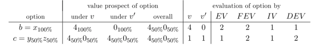
Being risk-averse, v and v0 both evaluate c at 1, below the expected value of 2. Al-though both options b and c have same value prospect, the source of uncertainty is normative for b and empirical for c. Table 4 shows how b and c are evaluated by four

value prospect of option evaluation of option by

option under v underv0 overall v v0 EV F EV IV DEV

b = x100% 4100% 0100% 450%050% 4 0 2 2 1 1

c = y_50%z_50% 4_50%0_50% 4_50%0_50% 4_50%0_50% 1 1 1 2 1 2

Table 4: The four meta-theories in the medical example

meta-valuations, namely the expected value theory EV and our three alternative value theories, the fully expectational, impartial, and dual expected value theories, denoted F EV , IV , and DEV , respectively. All four meta-theories de…ne overall value as the expected value of some object. That object –called the ‘focus of evaluation’–di¤ers: EV : Here the focus of evaluation is the option itself. So the overall value of an option is the average value of that option itself, i.e., 1₂4 + 1₂0 = 2 or 1₂1 + 1₂1 = 1, respectively.

F EV : Here the focus of evaluation is the world, i.e., the state of a¤airs after resolution of empirical uncertainty. Computing the average value of the world requires averaging not just across valuations in V (normative uncertainty), but also across worlds (empirical uncertainty). It may turn out –and does turn out for our two options – that only one dimension of averaging is needed, as only one source of uncertainty exists. Option b involves just normative uncertainty: it surely yields world x, of value 4 or 0. Option c involves just empirical uncertainty: it yields world y of sure value 4 or world z of sure value 0. For both options, the average value is 1₂4 +1₂0 = 2.

IV : Here the focus of evaluation is the value prospect of the option, which is 4_50%0_50% both times. So we must calculate how the value prospect 4_50%0_50% is evaluated on average by v and v0. But …rst, how does a valuation (v or v0) evaluate value prospects rather than options? Value prospects are evaluated like their corres-ponding options: v takes 450%050% to be the value prospect of option y50%z50%,

so that v(450%050%) reduces to v(y50%z50%) = 1; and v0 also takes 450%050% to be

the value prospect of y_50%z_50%, so that v0(4_50%0_50%) reduces to v0(y_50%z_50%) = 1. So the average value of 450%050% is 12v(450%050%) +12v0(450%050%) = 121 +

1 21 = 1.

For each option, we must calculate how the world’s value prospect is evaluated on average. Like for F EV , this requires averaging across both worlds and valuations – though for our options b and c one dimension of averaging drops out, as b has no empirical uncertainty while c has no normative uncertainty about evaluating value prospects of relevant worlds. Concretely, the option b = x_100%surely yields world x, whose value prospect 4_50%0_50% is evaluated at 1 by both (risk-averse) valuations v and v0, as seen earlier. So the average value is 1₂1 + 1₂1 = 1. The option c = y_50%z_50% either yields world y, whose value prospect 4_100% has value 4 under both v and v0; or yields world z, whose value prospect 0100% has value 0

under both v and v0. So the average value is 1₂4 +1₂0 = 2.

The risk-attitudinal rationale of each meta-theory. Each meta-theory has a focus of evaluation that is tailor-made for a particular risk attitude:

normatively risk-neutral normatively risk-averse

empirically risk-neutral F EV DEV

empirically risk-averse EV IV

Table 5: The risk attitudes of the four meta-theories in our example with risk-averse …rst-order theories

EV : Here the focus of evaluation – the option – captures empirical risk by being a lottery over worlds, but captures no normative risk. Through applying the (risk-averse) valuations in V to options, EV discounts for empirical risk, not for normative risk: it is averse to empirical risk only. Options without empirical risk like b are evaluated without discount, which explains why b gets higher value than c.

F EV : Here the focus of evaluation –the world –captures neither empirical, no norm-ative risk. Being riskless, worlds are evaluated without risk premium by the valuations in V. Hence F EV contains no risk premia: it is globally risk-neutral. This explains why both options b and c get the ‘high’value of 2.

IV : Here the focus of evaluation – the value prospect of the option – captures both empirical and normative risk. By applying the (risk-averse) valuations in V to the value prospect, F EV discounts for both types of risk, hence is globally risk-averse. This explains why both b (involving normative risk) and c (involving empirical risk) get the ‘low’value of 1.

DEV : Here the focus of evaluation –the value prospect of the world –captures norm-ative, but not empirical risk. By applying the (risk-averse) valuations in V to value prospects of worlds, DEV discounts for normative, but not empirical risk, hence is averse to normative risk only. This explains why b (involving normative risk) gets a higher value than c (involving empirical risk).

5.4 The new meta-theories de…ned formally

We start with the fully expectational value theory. It is not just ‘normatively expecta-tional’(like expected value theory EV ), but also ‘empirically expectational’. It averages

across worlds as well as valuations, hence across world/valuation combinations (x; v) in X _{V. Each combination (x; v) yields a value, v(x). It is weighted by the probability} of the combination, i.e., the probability a(x) of world x times the probability P r(v) of valuation v. Formally:

Fully expectational value theory (‘F EV ’). This meta-theory evaluates each option a 2 A by the expected value of the resulting world:

F EV (a) = X

(x;v)2X V

a(x)P r(v)

| {z }

prob. of (x;v)

v(x) (the ‘fully expectational value’ of a).

The impartial value theory operates at a di¤erent level: not the level of options (EV ) or worlds (F EV ), but the level of value prospects. This is possible because valuations v in V can be taken to evaluate not just options (and hence worlds, i.e., riskless options), but also value prospects. The value of a value prospect is simply the value of options having that value prospect. This de…nition however presupposes that (i) there exists an option in A with that value prospect under v, and (ii) any two such options are evaluated equally by v. Condition (i) essentially means that there are su¢ ciently many options in A, a typical decision-theoretic richness assumption. Condition (ii) holds for most or all natural …rst-order theories; it is the analogue of our Value-Prospect Principle, for …rst-order theories rather than meta-theories. We now formally state the background assumption (i)-(ii), followed by the de…nition which it enables:

Assumption: _{Hereafter, for each valuation v in V and value prospect p, there is a} corresponding option a in A whose value prospect pa;v is p, and any two such options

a have same value v(a).

De…nition 1 _{Under a valuation v in V, the value of a value prospect p – denoted} v(p) –is the value v(a) of options a 2 A whose value prospect under v is p, i.e., pa;v = p.

The ‘impartial value’is the average value of the value prospect:

Impartial value theory (‘IV ’). This meta-theory evaluates each option a 2 A by the expected evaluation of its value prospect:

IV (a) =X

v2V

P r(v)v(pa) (the ‘impartial value’ of a).

The dual expected value theory has yet another focus of evaluation, which is neither the option (EV ), nor the world (F EV ), nor the value prospect of the option (IV ), but the value prospect of the world. We thus form the average evaluation of the value prospect px, across worlds x and valuations v, i.e., across world/valuation combinations

(x; v). In this weighted average, each combination (x; v) is weighted by its probability, the product of the probabilities a(x) of x and P r(v) of v:

Dual expected value theory (‘_{DEV ’). This meta-theory evaluates each option a 2} A by the expected value of the value prospect of the world:

DEV (a) = X

(x;v)2X V

a(x)P r(v)

| {z }

prob. of (x;v)

v(px) (the dual expected value of a).

The distinctive mark of DEV is that it handles risk in the opposite way from EV . It applies valuations in V to world-value-prospects px(‘normative lotteries’) rather than

to the option a (an ‘empirical lottery’), thereby delegating the normative-risk attitude rather than the empirical-risk attitude to the …rst-order theories. Sections 6 and 7 will ‡esh this out formally.

5.5 The four meta-theories as ex-ante or ex-post theories

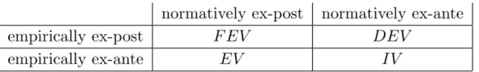
The four meta-theories are interpretable in terms of the famous ex-ante and ex-post approaches in ethics and aggregation theory under uncertainty.17 These approaches refer to whether competing evaluations of uncertain prospects (e.g., evaluations by di¤erent individuals) are aggregated before or after resolution of uncertainty. We work with two types of uncertainty –empirical and normative –and hence have four possible approaches, depending on whether we go ex-ante or ex-post on each type:

normatively ex-post normatively ex-ante

empirically ex-post F EV DEV

empirically ex-ante EV IV

Table 6: Interpreting the meta-theories as ex-ante or ex-post theories

F EV : The fully expectational value theory is a fully ex-post theory, as it aggregates evaluations of worlds x, i.e., riskless states of a¤airs.

IV : The impartial value theory is a fully ex-ante theory, as it aggregates evaluations of the value prospect pa, a state of unresolved empirical and normative uncertainty.

EV : The expected value theory is an empirically ex-ante theory, as it aggregates eval-uations of the option a, a state of unresolved empirical uncertainty.

DEV : The dual expected value theory is a normatively ex-ante theory, as it aggreg-ates evaluations of world-value-prospects px, i.e., states of unresolved normative

uncertainty.

Given the importance of the ex-ante and ex-post approaches in ethics, all four meta-theories are obvious ‘candidate theories’which deserve our attention.

5.6 In defence of the expectational form of IV

The impartial value theory IV has something in common with the classic expected value theory EV : the expectational or linear form. Indeed, IV builds a linear average

1 7

There is an on-going debate about which approach is more appropriate. For instance, Diamond’s (1976) famous objection against Harsanyi-type axiomatic utilitarianism assumes that ex-ante equality matters, something put into question by others (e.g., McCarthy 2006, 2008). The ex-ante and ex-post approaches to social well-being are compared by, e.g., Fleurbaey (2010), Fleurbaey and Voorhoeve (2016), and Fleurbaey and Zuber (2017).

of the v(pa)’s (v 2 V), not any geometric average or other non-linear compromise. While

EV ’s linearity causes the questionable neutrality to normative risk, IV ’s linearity does not cause any neutrality to normative or empirical risk. IV globally respects risk-attitudinal beliefs, as formally established later.

Aggregating the v(pa)’s in some non-linear way – in an attempt to (even better)

respect risk-attitudinal beliefs – could have the converse e¤ect of ‘overshooting’ the attitude, because of double-discounting. Why? Assume all v 2 V are risk-averse, and suppose in response the v(pa)’s (v 2 V) were aggregated sub-linearly, into

some overall value IV (a) < IV (a). The meta-theory IV can be more risk-averse than all valuations v 2 V. Each value v(pa) (v 2 V) already contains a risk premium

for all risk in a, empirical and normative, and hence so does IV (a). Reducing IV (a) further to IV (a) imposes another risk premium –a second one. One thereby becomes more risk-averse at the meta-level than is certainly correct at the …rst-order level.18

This said, we do not categorically insist on linearity. We insist on aggregating the v(pa)’s (v 2 V) rather than the v(a)’s (v 2 V), but we only propose a weighted

linear average as the most natural approach. Other approaches might be defensible, if they somehow avoid double-risk-discounting. One might more explicitly call IV the ‘linear impartial value theory’, which falls into the class of ‘generalized impartial value theories’, i.e., of meta-theories IV which de…ne the overall value of options a by aggregating the v(pa)’s in some (possibly non-linear) way.19

6

The impartial value theory addresses both objections

This section and the next formally substantiate previous arguments and claims. The present section shows how the impartial value theory avoids both problems of the ex-pected value theory raised in Section 3, after formally re-stating the principles proposed in Section 3.

6.1 Which meta-theories respect risk-attitudinal beliefs?

We now show that the impartial value theory IV satis…es Section 3’s two risk-attitudinal principles, while EV , F EV and DEV do not. Only IV forms a genuine comprom-ise between the risk attitudes of the competing valuations, thereby respecting attitudinal beliefs. The fully expectational value theory F EV blatantly violates risk-attitudinal beliefs, by being globally risk-neutral; and the ordinary and dual expected value theories EV and DEV respect risk-attitudinal beliefs w.r.t. just empirical risk (EV ) or just normative risk (DEV ).

But …rst, what are ‘risk-attitudes’of normative theories? Risk analysis has a long tradition in decision theory, where the bearers of risk-attitudes are usually individuals, not normative theories (e.g., Weirich 1986, 2004 Buchak 2013). Risk attitudes are often

1 8

By contrast, correcting the classic expected value EV (a) by subtracting a risk premium need not lead to double-risk-discounting, because EV (a) does not yet contain any premium for normative risk. Yet a non-linear aggregation of the v(a)’s has di¤erent problems, explained in Section 4.

1 9_{Formally, IV (a) = F (v(p}

a))v2V)for all a 2 A, for some …xed aggregation function F from RV to

de…ned through comparing the evaluation of risky objects with certain expectational evaluations. We adapt this approach to the realm of ethics and normative uncertainty. So we compare the value v(a) of a given option a under a given theory v with the expected value of the resulting world, P_x2Xa(x)v(x). Depending on whether v(a) matches, exceeds, or falls below that expectation, the evaluation of a is risk-neutral, -prone, or -averse. Formally:20

De…nition 2 _{A valuation v in V is risk-neutral (-averse, -prone) towards option} a 2 A if it evaluates a at (below, above) the expected value across worlds, i.e.,

v(a) = (<; >) X

x2X

a(x)v(x):

The risk premium for a or degree of risk-aversion towards a is the amount premv(a) by which a’s value falls below a’s expected resulting value:

premv(a) =

X

x2X

a(x)v(x) v(a):

A risk premium is a value discount due to risk. Its sign indicates whether there is risk aversion, neutrality, or proneness. Risk attitudes of meta-theories can be de…ned similarly, except that we must incorporate normative uncertainty by forming the expect-ation not just over worlds (empirical uncertainty), but also over valuexpect-ations (normative uncertainty). Formally:

De…nition 3 A meta-valuation V is risk-neutral (-averse, -prone) towards an option a 2 A if it evaluates a at (below, above) the expected value across worlds and valuations, i.e., V (a) = (<; >) F EV (a) = X (x;v)2X V a(x)P r(v) | {z } prob. of (x;v) v(x):

The risk premium for a or degree of risk aversion towards a is the amount by which a’s value falls below a’s fully expectational value:

P remV(a) = F EV (a) V (a):

In principle, a valuation or meta-valuation could be risk-averse towards some options and risk-neutral or -prone towards others. If such jumps are absent, we can talk of risk aversion, neutrality or proneness simpliciter :

2 0

This de…nition owes its plausibility to the assumption that theories in V measure value on an absolute scale. Accordingly, comparing value di¤erences is meaningful: a rise in value from 0 to 1 represents the same gain as one from 100 to 101. By contrast, a von-Neumann-Morgenstern function does not measure value on an absolute scale. There is intuitive compatibility between risk-aversion and evaluating lotteries by the expectation of a von-Neumann-Morgenstern function. (Indeed, economists often interpret agents as risk-averse if they evaluate money lotteries by the expectation of a concave von-Neumann-Morgenstern function.)

De…nition 4 _{A theory v in V or meta-theory V is risk-neutral (-averse, -prone)} if it is risk-neutral (-averse, -prone) towards all options with risky value prospect.21

Remark 1 The fully expectational value theory F EV is risk-neutral.

Just as we can apply valuations in V to value prospects rather than options (Section 5.4), so we can apply risk premia to value prospects rather than options:

De…nition 5 _{Given a valuation v in V, the risk premium for a value prospect p} or degree of risk aversion towards p, denoted premv(p), is the risk premium for

options a with value prospect pa;v = p.

Remark 2 premv(p) can be expressed as the amount by which p’s value falls below p’s

expectation:

premv(p) = Exp(p) v(p) =

X

k2R

p(k)k v(p):

We now formally state the Risk-Attitudinal Unanimity Principle of Section 3. We state the principle in two versions, depending on whether we take ‘risk attitude’to be a categorical or graded concept.

Risk-Attitudinal Unanimity Principle – qualitative version: _{If all v 2 V of} non-zero correctness probability P r(v) are risk-neutral (-averse, -prone), then the meta-theory V is also risk-neutral (-averse, -prone).

Risk-Attitudinal Unanimity Principle – quantitative version: For all options a 2 A, if all v 2 V of non-zero correctness probability P r(v) assign the same risk premium premv(pa) = r to a’s value prospect pa, then the meta-theory assigns that

same risk premium to a, i.e., P remV(a) = r.

Why does the quantitative principle assume a unanimous risk premium for a’s value prospect pa rather than for a? The reason is simple: the premv(a)’s (v 2 V)

are premia only for the empirical risk in a, while the premv(pa)’s (v 2 V) are premia

also for normative risk, since a’s value prospect pa also captures normative risk. By

contrast, at the meta-level the principle uses the option-level risk premium P remV(a),

as P remV(a) is already a premium for both types of risk, by being formed under

normative uncertainty. Stating the principle using option-level risk premia at both levels –…rst-order and meta –would have been implausible: it would have required that a unanimous premium for empirical risk be adopted as the meta-theoretic premium for empirical and normative risk. The point becomes obvious if a is empirically riskless, i.e., yields a sure world: then a’s …rst-order risk premia premv(a) (v in V) are unanimously

zero, yet a non-zero meta-theoretic premium may be justi…ed by normative uncertainty. Of the four meta-theories, only the impartial theory achieves the principle:

2 1

By the value prospect of an option a we here mean the theory-speci…c value prospect pa;v in case

of a …rst-order theory v in V, and the unconditional value prospect pa in case of a meta-theory. Why

does De…nition 4 exclude options with riskless value prospect from its quanti…cation? Requiring non-zero risk premia for essentially riskless options (i.e., requiring risk-aversion or -proneness towards such options) would be implausible, even for intuitively risk-averse or -prone theories.

Theorem 1 The Risk-Attitudinal Unanimity Principle, in its qualitative and quantit-ative version, is satis…ed by the impartial value theory IV , but can be violated by EV , F EV and DEV .

Intuitively, the fully expectational theory violates the principle by being always risk-neutral; the expected and dual expected value theories violate it by respecting the …rst-order risk attitudes w.r.t. just empirical risk (EV ) or just normative risk (DEV ); and the impartial value theory satis…es it by subjecting all risk to the valuations in V. Often there is risk-attitudinal uncertainty, i.e., heterogeneity in the risk attitudes across …rst-order valuations. In this heterogeneous case, the impartial value theory forms a linear compromise between the competing …rst-order risk attitudes:

Theorem 2 The degree of risk aversion of the impartial value theory IV towards an option a 2 A is the expected (‘average’) degree of risk aversion towards a’s value pro-spect:

P remIV(a) =

X

v2V

P r(v)premv(pa): (1)

Intuitively, IV has an ‘impartial’ risk attitude in the sense of a linear comprom-ise between …rst-order risk attitudes. IV thus satis…es Section 3’s Risk-Attitudinal Impartiality Principle, provided that principles is given a suitable linear interpretation. The meta-theoretic risk premium P remIV(a) is a compromise between the

prospect-level risk premia premv(pa) (v 2 V ), not the option-level risk premia premv(a) (v 2 V ).

This is a desirable feature, not a bug, because each premv(a) only accounts for empirical

risk in a, while each premv(pa) also accounts for normative risk.

6.2 Which meta-theories are based on the value prospect?

How do the new meta-theories perform w.r.t. the Value-Prospect Principle violated by the expected value theory? We give the answer in the next theorem, preceded by a formal re-statement of that principle.

Value-Prospect Principle: _{Options a; b 2 A with same value prospect p}a= pb have

same overall value V (a) = V (b).

Theorem 3 The Value-Prospect Principle is satis…ed by the impartial and fully ex-pectational value theories IV and F EV , but can be violated by the expected and dual expected value theories EV and DEV .

This positive result about IV holds trivially, as the impartial value of an option a is by de…nition determined by a’s value prospect. The positive result about F EV holds because, as shown in the appendix, the fully expectational value of an option a equals the expectation of a’s value prospect:

F EV (a) =X

k2R

7

Where and when do the meta-theories agree?

The expected and dual expected value theories EV and DEV lie between the fully expectational theory F EV and the impartial theory IV :

EV resembles F EV in its neutrality to normative risk, and IV in its impartial attitude to empirical risk.

DEV resembles F EV in its neutrality to empirical risk, and IV in its impartial attitude to normative risk.

Loosely speaking, each of EV and DEV is somewhere risk-neutral (like F EV ), and somewhere risk-attitudinally impartial (like IV ). Two theorems will substantiate this claim, thereby substantiating the perfect duality or symmetry between EV and DEV . The set of empirically riskless options is

Ae-riskless= fa 2 A : a(x) = 1 for some world x 2 Xg;

The set of options resulting in normatively riskless worlds is

An-riskless = fa 2 A : all v 2 V s.t. P r(v) 6= 0 agree at all x 2 X s.t. a(x) 6= 0g:

Theorem 4 The expected value theory EV matches

(a) the fully expectational value theory F EV at options in Ae-riskless (so is risk-neutral

towards such options),

(b) the impartial value theory IV at options in An-riskless (so has impartial risk

atti-tude towards such options in the sense of the average risk premium (1)). Theorem 5 The dual expected value theory DEV matches

(a) the fully expectational value theory F EV at options in An-riskless(so is risk-neutral

towards such options),

(b) the impartial value theory IV at options in Ae-riskless(so has impartial risk attitude

towards such options in the sense of the average risk premium (1)).

When do our meta-theories coincide at all options? This happens if risk-neutrality is certainly correct, i.e., only risk-neutral valuations have non-zero probability:

Theorem 6 All four meta-theories EV , F EV , IV and DEV coincide globally if each valuation in V of non-zero probability is risk-neutral.

This theorem even holds with an ‘if and only if’in all but certain arti…cial cases.

8

Concluding remarks

The classic expected value theory EV is one of four ‘expectational’ meta-theories, marked by di¤erent attitudes to normative and empirical risk (Theorems 1, 4, 5), and distinct in whether the aggregation of value follows an ex-ante or ex-post approach w.r.t. normative or empirical risk. We have conditionally defended the impartial value theory

IV , on the grounds that it respects impartially the …rst-order risk attitudes (Theorem 2) and is based solely on value information (Theorem 3). Our defence is conditional in di¤erent ways. First, IV presupposes as usual that normative uncertainty can be quanti…ed probabilistically and that value is numerically measurable and cross-theory comparable. Second, IV relies on a linear or expectational way to respect the …rst-order risk attitudes –it is ‘linearly impartial’. While we are open to non-linear versions of IV , we insist that IV ’s linear form does not cause any risk-neutrality –as opposed to classic EV , whose linear form causes the questionable neutrality to normative uncertainty.

A

Proofs

We here prove all results, in di¤erent order and based on many lemmas.

Lemma 1 The fully expectational value of an option a in A is the expectation of its value prospect:

F EV (a) = Exp(pa) ( =

X

k2R

kpa(k)):

Proof. For all options a in A,

F EV (a) = X (x;v)2X V a(x)P r(v)v(x) =X k2R X (x;v)2X V:v(x)=k a(x)P r(v)k =X k2R k X (x;v)2X V:v(x)=k a(x)P r(v) =X k2R kpa(k) = Exp(pa):

Proof of Theorem 3. IV and F EV satisfy the principle, by de…nition for IV and by Lemma 1 for F EV . EV and DEV can violate the principle: in Section 3.2’s example, pb = pc (= 450%050%) but EV (b) = 2 6= EV (c) = 1 and DEV (b) = 1 6= DEV (c) = 2.

Risk attitudes can be characterized in terms of evaluations of value prospects rather than options:

Lemma 2 _{A valuation v 2 V is risk-neutral (-averse, -prone) if and only if v(p) = (<,} >) Exp(p) for all value prospects p that are risky (i.e., do not assign probability one to any value).

Proof. We just show the claim for risk-neutrality, since the claims for risk-aversion and -proneness are analogous. First, consider a risk-neutral v 2 V and a risky value prospect p. We prove v(p) = Exp(p). Pick an a 2 A such that pa;v = p. By

risk-neutrality, v(a) =P_x2Xa(x)v(x). To show v(p) = Exp(p), we prove v(p) = v(a) and Exp(p) =P_x2Xa(x)v(x). The former holds because p = pa;v, and the latter because

Exp(p) =X k2R kp(k) =X k2R kpa;v(k) = X k2R k X x2X:v(x)=k a(x) =X k2R X x2X:v(x)=k a(x)k = X x2X a(x)v(x):

Conversely, let v(p) = Exp(p) for all risky value prospects p. Let a 2 A have risky value prospect pa;v. We must show v(a) = P_x2Xa(x)v(x). Letting p = pa;v, this

follows from the identity v(p) = Exp(p), because, as in the …rst part of the proof, v(p) = v(a) and Exp(p) =P_x2Xa(x)v(x).

Lemma 3 _{Every valuation v 2 V is risk-neutral towards options a 2 A whose value} prospect pa;v is riskless (i.e., assigns probability one to some value).

Proof. _{Let v 2 V and a 2 A such that p}a;v(k) = 1 for some k 2 R. We prove that

v is risk-neutral towards a, i.e., that v(a) = k (= F EV (a)). Pick any x 2 X such that a(x) 6= 0. Clearly, v(x) = k. Let b be the riskless option such that b(x) = 1. As pa;v = pb;v, we have v(a) = v(b), by assumption on valuations in V. Meanwhile

v(b) = v(x) = k. So v(a) = k.

Proof of Theorem 2. _{Consider an option a 2 A. Using Lemma 1,} F EV (a) = Exp(pa) = Exp(pa)

X v2V P r(v) =X v2V P r(v)Exp(pa): Now

P remIV(a) = F EV (a) IV (a)

=X v2V P r(v)Exp(pa) X v2V P r(v)v(pa) =X v2V P r(v) [Exp(pa) v(pa)] =X v2V P r(v)premv(pa):

Lemma 4 _{If a 2 A}n-riskless, then for all v 2 V such that P r(v) 6= 0 we have pa;v = pa

(whence v(a) = v(pa), applying v on both sides).

Proof. _{Let a 2 A}n-riskless. Then all pa;v with v 2 V and P r(v) 6= 0 coincide. Let p be

that common value prospect. It equals pa because, for all k 2 R,

pa(k) = X (x;v)2X V:v(x)=k a(x)P r(v) = X v2V:P r(v)6=0 P r(v) X x2X:v(x)=k a(x) = X v2V:P r(v)6=0 P r(v) pa;v(k) | {z } p(k) = p(k) X v2V:P r(v)6=0 P r(v) = p(k) 1 = p(k):

Proof of Theorem 4. _{(a) If a 2 A}e-riskless, say a(y) = 1 where y 2 X, then

F EV (a) = X (x;v)2X V a(x) |{z} =1(0)if x=(6=)y P r(v) v(x) |{z} =v(a)if x=y =X v2V P r(v)v(a) = EV (a):

(b) Let a 2 An-riskless. Then, assuming without loss of generality that P r(v) 6= 0 for

all v 2 V, EV (a) =X v2V P r(v)v(a) =X v2V P r(v)v(pa) = IV (a),

where the second identity uses Lemma 4.

Proof of Theorem 4. _{(a) Let a 2 A}n-riskless. Then:

DEV (a) = X (x;v)2X V a(x)P r(v)v(px) = X (x;v)2X V:a(x)6=0;P r(v)6=0 a(x)P r(v)v(px) F EV (a) = X (x;v)2X V a(x)P r(v)v(x) = X (x;v)2X V:a(x)6=0;;P r(v)6=0 a(x)P r(v)v(x):

To prove DEV (a) = F EV (a), it remains to show that v(px) = v(x), assuming a(x) 6= 0

and P r(v) 6= 0. As a 2 An-riskless and a(x) 6= 0, the world x (more precisely, the riskless

option identi…ed with x) belongs to An-riskless. So v(px) = v(x) by Lemma 4.

(b) If a 2 Ae-riskless, say a(y) = 1 where y 2 X, then

DEV (a) = X (x;v)2X V a(x) |{z} =1(0)if x=(6=)y P r(v)v(px) = X v2V P r(v)v(py) = IV (a):

Proof of Theorem 1. Write RUqual and RUquan for the qualitative and quantitative

versions of the Risk-Attitudinal Unanimity Principle. Let ~_{V = fv 2 V : P r(v) 6= 0g.} Claim 1: IV satis…es RUqual.

Assume all v 2 ~V are riskaverse; the proof is analogous for riskneutrality or -proneness. Consider any a 2 A with risky value prospect pa. We must show that IV

is risk-averse towards a, i.e., that IV (a) < F EV (a). Note IV (a) =X v2V P r(v)v(pa) = X v2 ~V P r(v)v(pa):

In the last expression, each v(pa) is below Exp(pa) by v’s risk-aversion and Lemma 2.

So IV (a) <X v2 ~V P r(v)Exp(pa) = Exp(pa) X v2 ~V P r(v) = Exp(pa) 1 = F EV (a),

where the last equality uses Lemma 1. This proves IV (a) < F EV (a). Claim 2: IV satis…es RUquan.

This claim is a special case of Theorem 2, proved above. Claim 3: F EV can violate RUqual and RUquan.

This claim is trivial. Just choose X; A; V and P r such that the v 2 ~V are all risk-averse (or all risk-prone); as F EV is risk-neutral, RUqual is violated. If we moreover

let all v 2 ~V have same non-zero degree of risk aversion premv(pa) towards the value

prospect paof some option a 2 A –e.g., by letting ~V be singleton –then RUquan is also

violated, because P remF EV(a) = 0.

Claim 4: EV can violate RUqual.

Choose any X; A; V and P r such that (i) all v 2 ~V are risk-averse, and (ii) some world y 2 X is evaluated di¤erently by at least two valuations in ~V. We prove that EV is not risk-averse. Let a be the option which certainly yields y. So a(x) = 1(0) if

x = (6=)y. Hence, _X

x2X

Now EV (a) =X v2V P r(v)v(a) =X v2V P r(v)X x2X a(x)v(x) by (2) = X (x;v)2X V a(x)P r(v)v(x) = F EV (a):

As EV (a) = F EV (a), EV is risk-neutral towards a. So EV is not globally risk averse, noting that a’s value prospect pais risky as a (i.e., the world y) is evaluated di¤erently

by di¤erent valuations in ~_V.

Claim 5: EV can violate RUquan.

Choose any X; A; V and P r such that there is a world y 2 X for which (i) v(y) is not the same for all v 2 ~V, and (ii) all v 2 ~V assign the same risk premium to y’s value prospect, denoted premv(py) prem(py). Such a choice is possible, namely by

constructing a set of valuations V in three steps (and letting P r(v) 6= 0 for all v 2 V): …rst, …x a y 2 X and …x how the v 2 V evaluate worlds (riskless options), taking care that y is evaluated di¤erently; second, …x a function prem of value prospects p, where prem(p) is zero if and only if p is riskless (prem(p) will become the risk premium for p); third, extend each v 2 V to risky options a by de…ning v(a) as

v(a) = X

x2X

a(x)v(x) prem(pa;v) = Exp(pa;x) prem(pa;x);

the di¤erence between a’s expected world value and a premium for the empirical risk. Each v 2 V assigns to each value prospect p the value v(p) = Exp(p) prem(p) and hence the risk premium premv(p) = Exp(p) v(p) = prem(p) (which con…rms the ‘risk

premium’interpretation given to the function prem).

Now let a be the riskless option which surely yields y. By (i), a’s value prospect pa is risky. Each premv(pa) is the same for all v 2 V, namely prem(pa). So RUquan

would require that P remEV(a) = prem(pa). Yet P remEV(a) 6= prem(pa), because

prem(pa) 6= 0 (as pa is risky), while P remEV(a) = 0 (as EV is risk-neutral towards

empirical-riskless options like a, by Theorem 4(a)). Claim 6: DEV can violate RUqual.

Choose any X; A; V and P r such that some risk-averse ~v 2 V is surely correct: P r(~v) = 1 (no normative uncertainty). So ~_{V = f~vg. Hence trivially all v 2 ~V are} risk-averse. So RUqual requires of DEV to be risk-averse. But by Theorem 5(a) DEV

globally coincides with the risk-neutral meta-theory F EV , as A = An-riskless.

Claim 7: DEV can violate RUquan.

Choose X; A; V and P r just as in Claim 6’s proof. To see why RUquan is violated,

pick any a 2 A with risky value prospect pa. As ~V = f~vg, trivially premv(pa) is the

same for all v 2 V. So RUquan requires of DEV that P remDEV(a) = prem~v(pa). Yet

prem~v(pa) 6= 0 (as ~v is risk-averse and pais risky) while P remDEV(a) = 0 (as DEV is