HAL Id: halshs-00277379
https://halshs.archives-ouvertes.fr/halshs-00277379
Submitted on 6 May 2008
HAL is a multi-disciplinary open access
archive for the deposit and dissemination of sci-entific research documents, whether they are pub-lished or not. The documents may come from teaching and research institutions in France or abroad, or from public or private research centers.
L’archive ouverte pluridisciplinaire HAL, est destinée au dépôt et à la diffusion de documents scientifiques de niveau recherche, publiés ou non, émanant des établissements d’enseignement et de recherche français ou étrangers, des laboratoires publics ou privés.
Business surveys modelling with Seasonal-Cyclical Long
Memory models
Laurent Ferrara, Dominique Guegan
To cite this version:
Laurent Ferrara, Dominique Guegan. Business surveys modelling with Seasonal-Cyclical Long Memory models. 2008. �halshs-00277379�
Documents de Travail du
Centre d’Economie de la Sorbonne
Business surveys modelling with
Seasonal-Cyclical Long Memory models
Laurent F
ERRARA,Dominique G
UEGANBusiness surveys modelling
with Seasonal-Cyclical Long Memory models
Ferrara L. ∗and Guégan D. †2nd May 2008
Abstract:
Business surveys are an important element in the analysis of the short-term economic situation because of the timeliness and nature of the information they convey. Especially, surveys are often involved in econometric models in order to provide an early assessment of the current state of the economy, which is of great interest for policy-makers. In this paper, we focus on non-seasonally adjusted business surveys released by the European Commission. We introduce an innovative way for modelling those series taking the persistence of the seasonal roots into account through seasonal-cyclical long memory models. We empirically prove that such models produce more accurate forecasts than classical seasonal linear models.
Keywords:
Euro area, nowcasting, business surveys, seasonal, long memory. JEL Classification:
C22, C53, E32.
∗Banque de France et Centre d’Economie de la Sorbonne, Université Paris 1 – Panthéon – Sorbonne, e-mail:
[email protected]. The views expressed herein are those of the author and do not necessarily reflect those of the Banque de France.
†Centre d’Economie de la Sorbonne, Université Paris 1 – Panthéon – Sorbonne, UMR 7184, e-mail:
1
Introduction
Early assessment of the current state of the economy is important for policy-makers. Unfor-tunately, reference figures used to assess economic growth are those of the quarterly national accounts which are released with a substantial delay. For example, euro area GDP figures are re-leased by Eurostat around 45 days after the end of the reference quarter. The same delay applies for the industrial production index. Therefore, short-term analysts have developed econometric tools that exploit the information content of timely updated monthly indicators in order to pro-vide with early estimates of GDP growth. This exercise is often referred to as ’nowcasting’ in the recent litterature (see for example Ferrara, 2007, or Angelini et al., 2008).
In this respect, business surveys are an important element in the analysis of the short-term eco-nomic situation because of the timeliness and nature of the information they convey. Indeed, business surveys are available from the end of the reference month and are rarely revised. In this paper, we focus on non-seasonally adjusted Euro-zone business surveys released by the European Commission. We show that those time series exhibit long-range dependence in the seasonal roots and we introduce an innovative way of modelling those series by taking this persistence into account through Seasonal-Cyclical Long Memory [SCLM] models. The class of SCLM models is an extension of the Fractionally Integrated model introduced by Granger and Joyeux (1980) and Hosking (1981) often used in macroeconomics (see for example Baillie, 1996, for a review). Such models possess the ability to take simultaneously into account long range dependence and cyclical behaviour. SCLM models have been introduced by Robinson (1994) and studied by Arteche and Robinson (2000). It turns out that those models are flexible enough to nest a lot of seasonal or cyclical fractionally integrated models that have been proposed in the literature.
In this paper, we describe the general class of SCLM models in section 1. Then, in section 2, we propose an innovative application of SCLM models to business surveys in the euro area. We com-pare this kind of models with classical seasonal linear models, based on Seasonal Auto-Regressive Integrated Moving-Average (SARIMA) models, in terms of predictive content. We empirically prove that SCLM models produce more accurate forecasts than SARIMA models.
2
SCLM models
In this section we present models referred to as Seasonal-Cyclical Long Memory models, that include generalized long memory processes and seasonal long memory processes. Such kinds of models are well appropriate for data exhibiting short term-dependent (seasonal or non-seasonal) ARMA components and slowly decaying auto-correlation at periodic lags. The use of frac-tional seasonal degrees allows to take seasonal fluctuations into account while avoiding over-differentiation. The autocorrelation function [ACF] of a seasonal fractionally integrated model displays an hyperbolic decay at seasonal lags, rather than the slow linear decay characterizing the conventional seasonally integrated model. Indeed, we generally observe on the ACF of real data set a superposition of hyperbolically damped sin waves.
In the spectral domain, a peak in the spectral density at a given frequency λ indicates a cycle of period 2π
λ in the process. More generally, a seasonal process (Xt)t presents several peaks in
the spectral density located at the seasonal frequencies λh = 2πh
s , h = 1, . . . , [s/2], where s is
monthly data and s = 52 for weekly data), and [s/2] denotes the integer part of s/2. Seasonal long memory models allow a representation of the spectral density showing a singularity at zero or at any frequency ω, 0 < ω ≤ π, such that:
f (ω + λ) ∼ C|λ|−2d, as, λ → 0, |d| < 1/2, (1) where C is a positive constant and d is any real lying on the interval ] − 0.5, 0.5[. When f (λ) satisfies the equation (1) for every seasonal frequency ω = ωh, h = 1, 2, · · · , [s/2], possibly with
the memory parameter, d, varying across h, we say that the process has a seasonal long memory behavior. However, for non-seasonal time series, like annual data, equation (1) holds for a single frequency ω ∈]0, π] as well as eventually for ω = 0.
Without loss of generality, we assume that the process (Xt)t is a zero-mean stationary process
with finite variance. The SCLM model for Xt is defined as follows:
(I − B)d0 k−1Y i=1 (I − 2B cos λi+ B 2 )di (I + B)dk Xt= εt, (2)
where B is the backshift operator, where for i = 1, · · · , k − 1, di ∈ R and λican be any frequency
between 0 and π. The innovations (εt)thave continuous and positive spectrum. We say that the
process (Xt)t is integrated of order di at frequency λi, Iλi(di), for i = 0, 1, 2, · · · , k, λ0 = 0 and
λk= π. Generally, in applications, the innovations (εt)t are supposed to follow a short-memory
stationary ARMA process.
The general representation (2) nests a lot of seasonal or cyclical fractional models introduced in the literature that are competitive to take those specific behaviors into account. Among the papers dealing with theoretical and empirical aspects of those models we refer to Gray, Zhang and Woodward (1989), Porter-Hudak (1990), Ray (1993), Hassler (1994), Giraitis and Leipus (1995), Woodward, Cheng and Gray (1998) Arteche and Robinson (2000), Ferrara and Guégan, (2000, 2001a, 2001b, 2006), Gil-Alana (2001, 2006), Guégan (2000, 2003), Arteche (2003), Ol-hede, McCoy and Stephens (2004), Chan and Palma (2005), Reisen, Rodriguez and Palma (2006) or Ferrara, Guégan and Lu (2008) for instance.
3
A SCLM modelling for business surveys
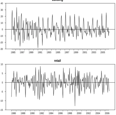
We focus on non-seasonally business surveys for the euro area released each end of month by the European Commission. Several economic sectors are covered by those surveys: Industry, build-ing, retail trade, services and consumers. All the countries of the European Union are considered, as well as the euro area and the EU27 as a whole. It turns out that not all the opinion surveys present a seasonal pattern. Based on the shape of the periodogram of the differenced series, we retain two sectors with marked seasonality, namely the building and retail trade sectors at the euro area aggregated level (see Figure 1).
Let us note (X1
t)t the first item of the construction survey (trend activity over recent months)
and (X2
t)t the fifth item of the retail survey (employment expectations), at the euro area level
from January 1985 to December 2006. The main interest of economic analysts concerns the variations of the surveys from one month to the other. Therefore, in this paper, we consider the first order differencing of the raw series, denoted (Y1
t )tand (Y 2 t )tdefined by Ytj = X j t− X j t−1, for
j = 1, 2. Moreover, by cancelling the signal in the low frequencies, this differencing filter allows to focus only on the seasonal variations of the series, which is of main interest in this study. Both first order differenced surveys are presented in Figure 1. We observe that these series are centered around zero and dominated by a seasonal component.
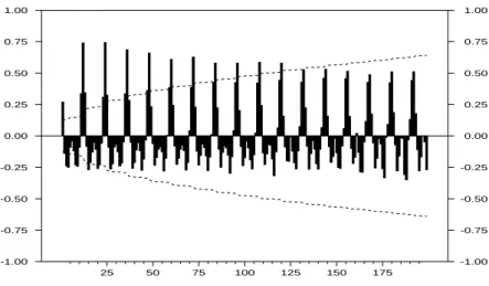
As regards the building survey, the excess kurtosis of the series is significantly equal to zero (dKu = 0.4437), but the series is asymmetric, the skewness being estimated at cSk = 0.3706. The ACF of the series (Figure 2) shows evidence of a strong seasonal pattern with a cycle of period 12 months, but also a shorter cycle with negative auto-correlations seems to be present. The ACF decreases very slowly as the lags increase, indicating the presence of strong persistence inside the data. The raw periodogram in Figure 3 exhibits two marked peaks at the seasonal frequencies π/6 and π/3, corresponding respectively to cycles of period 12 months and 6 months. The peaks located at the other seasonal frequencies π/2, 2π/3, 5π/6 and π present a weaker amplitude but are marked anyway. This picture suggests a higher degree of persistence for the two first seasonal frequencies.
As regards the retail trade surveys, the excess kurtosis is non-null at the classical confidence level 1 − α = 0.95 (dKu = 0.7208), implying thus non-Normality through a Jarque-Bera test. Moreover, this property of non-Normality is reinforced by a negative skewness ( cSk = −0.3406), non-null at the usual confidence level. Those statistics indicate that negative large shocks are more frequent than positive ones. The ACF (Figure 4) is quite different from the previous one, in the sense that we do not observe a slow decay, but we have rather a persistence in a cycle of period around 12 months. Moreover, other cycles seem to be present, but the ACF is too noisy
building 1985 1987 1989 1991 1993 1995 1997 1999 2001 2003 2005 -30 -20 -10 0 10 20 30 40 retail 1986 1988 1990 1992 1994 1996 1998 2000 2002 2004 2006 -15 -10 -5 0 5 10
Figure 1: First order difference opinion surveys: Trend of activity over recent months in the construction (top) and Employment expectations in the retail sector (bottom)
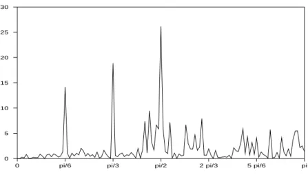
to be interpreted clearly, so we turn to the spectral domain. The spectral density of the series estimated by the raw periodogram is presented in Figure 5. Three main peaks emerge from this picture, located at the three first seasonal frequencies, namely π/6, π/3 and π/2. This indicates the presence of three cycles of period, respectively, 12, 6 and 4 months. It is noteworthy that the 4-month period cycle seems to be the most persistent.
The previous described stylized facts suggest that the use of a SCLM model described in equation (2) seems adequate to explain the dynamics of these two series. We use a purely seasonal model with six frequencies, but without short-term component. Thus, for j = 1, 2, we use the following modelling: Π5 i=1(I − 2 cos(iπ/6)B + B 2 )di (I + B)d6 Xtj = εt, (3)
where (εt)t is a stationary process. Pseudo-maximum likelihood estimates of the parameters of
model (3), over the whole period (Feb. 1985 - Dec. 2006), are provided in Table 1.
Building (X1 t) Retail (X 2 t) i λˆ i dˆi dˆi 1 π/6 0.5160 0.2237 2 π/3 0.5081 0.1929 3 π/2 0.4006 0.4379 4 2π/3 0.4731 0.1912 5 5π/6 0.4022 0.1986 6 π 0.1654 0.1764
Table 1: Parameter estimates of the SCLM models fitted to the building survey in differences
As regards the building survey (second column of Table 1), the first two memory parameters are slightly greater than 0.5 (indicating thus a non-stationary behavior), while the other components are not. Especially, we observe on both series that movements associated with the frequency π are not strongly persistent. Concerning the retail survey (third column of Table 1), the memory parameter associated to the cycle of period four months (λi = π/2) is the highest but it is still
stationary. Other parameters are lower but non-null.
As a benchmark we fit also a classical linear SARIMA model to both series, over the whole sample (Feb. 1985 - Dec. 2006). As regards the building survey (X1
t)t, the more parcimonious
model that allows to whiten the residuals is the SARIMA(3, 0, 0)(2, 1, 0)12, without constant in
the equation. The estimated model is the following:
(I − B12)(I − 0.2249B − 0.2974B2− 0.1325B3)(I − 0.5421B12− 0.1888B24)Xt1 = εt. (4)
All the estimates are non-null using a Student test with α = 0.05 and the estimated residual standard error is equal to 5.36.
Concerning the retail trade survey (X2
t)t, the more parcimonious model that allows to whiten
the residuals is the SARIMA(3, 0, 0)(3, 1, 0)12, without constant in the equation. The estimated
model is the following:
(I − B12)(I − 0.4602B − 0.3824B2− 0.2204B3)(I − 0.6720B12− 0.4687B24− 0.2842B36)Xt2 = εt.
All the estimates are non-null using a Student test with α = 0.05 and the estimated residual standard error is equal to 3.22.
We describe now the forecasting experience. We use a rolling procedure by using first the learn-ing set from the beginnlearn-ing of the series, in January 1985, to December 1999 and we forecast over three years (h = 36) using both models. Then we extend progressively the learning set, one year by one year, untill December 2003, in order to provide forecasts to December 2006, the last point of our analysis. That is, we can assess the forecasting performances over 5 various forecasting horizons (2000-2002, 2001-2003, 2002-2004, 2003-2005 and 2004-2006). Therefore, for each forecasting horizon we can compute the root-mean-squared error (RMSE hereafter) of each model. To have a quick summary of the results, we compute the ratios of the RMSE, by dividing the RMSE from the SCLM model by the one from the SARIMA model. Thus, a ratio lower than one indicates a better forecasting performance of the SCLM model. Results are presented in the Table 2. Building (X1 t) Retail (X 2 t) 2000-2002 0.80 0.85 2001-2003 0.69 0.83 2002-2004 0.87 0.87 2003-2005 0.96 0.86 2004-2006 1.02 0.88
Table 2: Ratios of the RMSE for the SCLM model over the RMSE the SARIMA model
From these results, we note that the SCLM model provides systematically better forecasting results for all horizons (except over 2004-2006 for the building survey). The gain is more sig-nificative for the retail survey, while the gain depends strongly on the forecast horizon for the building survey. Those results are interesting and point out the interest of such fractional models. However, this study should be generalized to a greater number of opinion surveys, especially in the presence of a low frequency component.
4
Conclusion
In this paper we have put forward an innovative approach for modelling non-seasonal adjusted business surveys through Seasonal-Cyclical Long Memory models. Those models allow to take the persistence of seasonal roots into account. We prove empirically that SCLM models can be very competitive in terms of forecasting by comparison with classical linear models. Consequently, this approach could lead to a better approximation in the seasonal adjustment procedures when the series has to be predicted, implying thus a more accurate economic assessment for policy-makers. SCLM models have to be used at a larger scale in a forecasting competition with SARIMA models, but also with other non-linear seasonal models like for instance the Periodic Auto-Regressive model (Franses and Ooms, 1997).
References
[1] Angelini, E., Camba-Mendez, G. Giannone D., Reichlin, L. and Ruenstler, G., Short-term forecasts of euro area GDP growth, Discussion Paper Series No. 6746, CEPR.
[2] Arteche J. (2003), Semi-parametric robust tests on seasonal or cyclical long memory time series, Journal of Time Series Analysis, 23, 251 - 285.
[3] Arteche J., Robinson P.M. (2000), Semiparametric inference in seasonal and cyclical long memory processes, Journal of Time Series Analysis, 21, 1 - 25.
[4] Baillie, R. (1996), Long memory processes and fractional integration in econometrics, Jour-nal of Econometrics, 73, 5 - 59.
[5] Chan, N.H., and W. Palma (2005), Efficient estimation of seasonal long range dependent processes, Journal of Time Series Analysis, 26, 863 - 892.
[6] Ferrara, L. (2007), Point and interval nowcasts of the Euro area IPI, Applied Economics Letters, Vol. 14, No. 2, pp. 115-120.
[7] Ferrara, L. and D. Guégan (2000), Forecasting financial time series with generalized long memory processes, in Advances in Quantitative Asset Management, pp. 319-342, C.L. Dunis ed., Kluwer Academic Publishers.
[8] Ferrara, L. and Guégan, D. (2001a), Forecasting with k-factor Gegenbauer processes: Theory and applications, Journal of Forecasting, 20, 581-601.
[9] Ferrara, L. and D. Guégan (2001b), Comparison of parameter estimation methods in cyclical long memory time series, in Developments in Forecast Combination and Portfolio Choice, Chapter 8, C. Dunis, J. Moody and A. Timmermann (eds.), Wiley, New York.
[10] Ferrara, L. and Guégan, D. (2006), Fractional seasonality : Models and applications to eco-nomic activity in the Euro area, paper presented at the Conference for Seasonality, Seasonal Adjustement and their implications for Short-Term Analysis and Forecasting, organized by Eurostat, Luxembourg, May 2006 et CES-AC Working Paper, No. 2 - 2006.
[11] Ferrara, L., Guégan, D. and Z. Lu (2008), Testing fractional order of long memory processes: A MonteCarlo study, CES Working Paper No. 2008.12, University Paris 1 Panthéon -Sorbonne.
[12] Franses, P.H., and Ooms M. (1997), A periodic long memory model for quartely UK inflation, International Journal of Forecasting, 13, 117 - 126.
[13] Gil-Alana L.A. (2001), Testing stochastic cycles in macro-economic time series, Journal of Time Series Analysis, 22, 411 - 430.
[14] Gil-Alana L.A. (2006), Testing seasonality in the context of fractionally integrated processes, Annales d’Economie et de Statistique, 81,69- 91
[15] Giraitis, L., Leipus R. (1995), A generalized fractionally differencing approach in long mem-ory modelling, Lithuanian Mathematical Journal, 35, 65 - 81.
[16] Granger C.W.J. and R. Joyeux (1980), An introduction to long memory time series models and fractional differencing, Journal of Time Series Analysis, 1, 15 - 29.
[17] Gray, H.L., Zhang, N.-F. and Woodward, W.A. (1989), On generalized fractional processes, Journal of Time Series Analysis, 10, 233-257.
[18] Guégan, D. (2000), A new model : the k-factor GIGARCH process, Journal of Signal Processing, 4, 265-271.
[19] Guégan, D. (2003), A prospective study of the k-factor Gegenbauer process with het-eroscedastic errors and an application to inflation rates, Finance India, 17, 1 - 21.
[20] Hassler, U. (1994), Misspecification of long memory seasonal time series, Journal of Time Series Analysis, 15, 19 - 30.
[21] Hosking J.R.M., (1981), Fractional differencing, Biometrika, 68, 1, 165-176.
[22] Olhede S.C., McCoy E.J., Stephens D.A. (2004), Large-sample of the periodogram estimator of sesonally persistent processes, Biometrika, 91, 613 - 628.
[23] Ray B.K. (1993), Long-range forecasting of IBM product revenues using a seasonal fraction-ally differenced ARMA model, International Journal of Forecasting, 9, 255 - 269.
[24] Reisen, V., Rodrigues, A. and Palma, W. (2006), Estimating Seasonal Long Memory Pro-cesses. A Monte Carlo Study, Journal of Statistical Computation and Simulation, 76, 4, 280-316.
[25] Robinson P.M. (1994), Efficient tests of non-stationary hypotheses, Journal of the American Statistical Association, 89, 1420 -1457.
[26] Woodward, W.A., Cheng Q.C. and Gray H.L. (1998), A k-factor GARMA long-memory model, Journal of Time Series Analysis, 19, 5, 485-504.
25 50 75 100 125 150 175 -1.00 -0.75 -0.50 -0.25 0.00 0.25 0.50 0.75 1.00 -1.00 -0.75 -0.50 -0.25 0.00 0.25 0.50 0.75 1.00
Figure 2: ACF of the building survey (trend activity over the recent months) in difference
0 pi/6 pi/3 pi/2 2 pi/3 5 pi/6 pi
0 80 160 240 320 400 480 560 640
Figure 3: Raw periodogram of the building survey (trend activity over the recent months) in difference
25 50 75 100 125 150 175 -1.00 -0.75 -0.50 -0.25 0.00 0.25 0.50 0.75 1.00 -1.00 -0.75 -0.50 -0.25 0.00 0.25 0.50 0.75 1.00
0 pi/6 pi/3 pi/2 2 pi/3 5 pi/6 pi 0 5 10 15 20 25 30