HAL Id: hal-00980125
https://hal.archives-ouvertes.fr/hal-00980125
Preprint submitted on 17 Apr 2014
HAL is a multi-disciplinary open access
archive for the deposit and dissemination of
sci-entific research documents, whether they are
pub-lished or not. The documents may come from
teaching and research institutions in France or
L’archive ouverte pluridisciplinaire HAL, est
destinée au dépôt et à la diffusion de documents
scientifiques de niveau recherche, publiés ou non,
émanant des établissements d’enseignement et de
recherche français ou étrangers, des laboratoires
On the relationship between the prices of oil and the
precious metals: Revisiting with a multivariate
regime-switching decision tree
Philippe Charlot, Vêlayoudom Marimoutou
To cite this version:
Philippe Charlot, Vêlayoudom Marimoutou. On the relationship between the prices of oil and the
precious metals: Revisiting with a multivariate regime-switching decision tree. 2014. �hal-00980125�
EA 4272
On the relationship between the
prices of oil and the precious metals:
Revisiting with a multivariate
regime-switching decision tree
Philippe Charlot*
Vêlayoudom Marimoutou**
2014/13
(*) LEMNA - Université de Nantes
(**) Aix-Marseille School of Economics
Laboratoire d’Economie et de Management Nantes-Atlantique
Université de Nantes
Chemin de la Censive du Tertre – BP 52231
44322 Nantes cedex 3 – France
www.univ-nantes.fr/iemn-iae/recherche
D
o
cu
m
en
t
d
e
T
ra
va
il
W
o
rk
in
g
P
ap
er
On the relationship between the Prices of oil and the Precious
Metals: Revisiting with a Multivariate Regime-Switching Decision
Tree
✩Philippe Charlota,∗, Vˆelayoudom Marimoutoub
a
LEMNA, University of Nantes
Chemin de la Censive du Tertre - BP 52231, 44322 Nantes Cedex 3, France
b
Aix-Marseille University (Aix-Marseille School of Economics), CNRS & EHESS 2 rue de la Charit´e, 13236 Marseille cedex 02, France
Abstract
This study examines the volatility and correlation and their relationships among the euro/US dollar exchange rates, the S&P500 equity indices, and the prices of WTI crude oil and the precious metals (gold, silver, and platinum) over the period 2005 to 2012. Our model links the univariate volatilities with the correlations via a hidden stochastic decision tree. The ensuing Hidden Markov Decision Tree (HMDT) model is in fact an extension of the Hidden Markov Model (HMM) introduced byJordan et al. (1997). The architecture of this model is the opposite that of the classical deterministic approach based on a binary decision tree and, it allows a probabilistic vision of the relationship between univariate volatility and correlation. Our results are categorized into three groups, namely (1) exchange rates and oil, (2) S&P500 indices, and (3) precious metals. A switching dynamics is seen to characterize the volatilities, while, in the case of the correlations, the series switch from one regime to another, this movement touching a peak during the period of the Subprime crisis in the US, and again during the days following the Tohoku earthquake in Japan. Our findings show that the relationships between volatility and correlation are dependent upon the nature of the series considered, sometimes corresponding to those found in econometric studies, according to which correlation increases in bear markets, at other times differing from them.
Keywords: Multivariate GARCH; Dynamic correlations; Regime switching; Hidden Markov
✩The authors thank Zakaria Moussa for the dataset provided for this work and Allan Bailur for useful
com-ments. This research has been supported partially by the Aix Marseille School of Economics. Any errors and shortcomings in the paper remain our own responsibility.
∗Corresponding author.
Email addresses: ph.charlot@gmail.com (Philippe Charlot), velayoudom.marimoutou@univ-amu.fr
Decision Tree.
JEL Classification: C32, C51, G1, G0.
1. Introduction
The relationship between volatility and correlation has been widely studied. The overall conclusion of many studies, mainly based on international equity returns or indices, is that correlations are not only time-varying, but there is also a particular connection between the two statistical measures. Correlation appears indeed to be higher during Bear markets. That suggests that the degree of dependence between series rises as stock values fall.
This asymmetric relationship between state of the market and correlations cannot be analyzed simply by comparing estimated values. A first set of studies have been undertaken using extreme value theory (Longin and Solnik (2001)), and a quantile correlation measure to a portfolio allocation (Campbell et al. (2002)) whileAng and Bekaert (2002) estimate a Markov-switching multivariate-normal model. A second set of studies have proposed statistical methods to test the presence of asymmetric correlations (seeAng and Chen (2002) andHong et al. (2006)). In this paper, we examine the connections between univariate volatility and correlations between euro/US dollar exchange rate, S&P500 index, oil and precious metals from January 2005 to 19 October 2012, covering a period which includes the subprime crisis. In contrast to the previous studies, our method is based on a two level Hidden Markov Decision Tree (HMDT) proposed byJordan et al. (1997). The first level discriminates between low and turbulent volatility while the second determine the correlations. Then, a probabilistic relationship between the two levels is established.
The paper is organized as follows. Section2 provides a brief review of the existing literature on the dynamics of exchange rates, S&P500 indices, and prices of oil and the precious metals. In section 3 we present our model. Section 4 contains our findings, Section 5 presents our discussions and conclusions, and sets out areas for further research.
2. Review
The existing specialist literature on metals commodities and oil markets can be considered on two levels. At the first level, it consists of an analysis of the univariate characteristics of the series, while at the second level the analysis covers a multivariate setting, and attempts to explain the linkages between these variables.
Exchange rates and equity indices are the main field of application for volatility models. In that context, the autoregressive conditional heteroskedasticity (ARCH) model ofEngle (1982) and its generalised counterpart (GARCH), proposed byBollerslev (1986), are among the most widely used specifications in the empirical literature. The analysis ofLunde and Hansen (2005) points to GARCH(1,1) as the most favoured specification for a study of the volatility of exchange rates.
The litterature on oil price fluctuations is substantial. The main recent contributions regarding oil are listed in the introduction of the paper byWang and Wu (2012). While these studies use GARCH type models for the volatility of oil prices, consensus about the dynamics seems hard to reach. The determinants of oil market price volatility are mainly due to macroeconomic factors but also speculative and exogenous geopolitical events (seeHamilton (2009)). Studies conclude that a simple GARCH(1,1) can reproduce oil series (see Cheong (2009), Agnolucci (2009)), while others consider that CGARCH model and FIGARCH (Kang et al. (2009)) or a Markov-switching GARCH model (seeNomikos and Pouliasis (2011)) are more suitable.
In recent years, numerous studies on the precious metals have been published, and they underline the importance of the dynamics of the volatility of their prices: time-dependence and GARCH effects in the spot price of gold and silver (Akgiray et al. (1991),Schwartz (1997)), non-linear models perform better than a random-walk model (Escribano and Granger (1998)), day effects and daily seasonality (Lucey and Tully (2006b)). In the case of platinum,Adrangi and Chatrath (2002) find the strong evidence of nonlinear dependence, which can be explained by ARCH-type pro-cesses.
More recently, some studies have investigated the potential existence of structural changes and long memory in precious metals prices (Arouri et al. (2012),Cochran et al. (2012)). However, the distinction between a true switching model and the long-memory property is far from clear in the current econometric literature (seeDiebold and Inoue (2001) andGranger and Hyung (2004) and alsoCheung and Lai (1993) for a discussion on long memory in gold returns).
At a multivariate level, co-movement of commodity prices was examinate byDeb et al. (1996) whose results suggest the presence of excess co-movement in the univariate setup, but not in the multivariate case. Pindyck and Rotemberg (1990) found that unrelated commodities tend to move together, but this conclusion was subsequently disproved byCashin et al. (1999). In the case of metals, Chen (2010), investigated the relationship between precious and indus-trial metals from 1900 to 2007, and found the consequences of a shock on a metal’s price
depends on the category to which that metal belongs, and that any spill-over effects are only marginal. Among precious metals, gold and silver serve different industrial purposes, while at a financial level the two metals can be substituted one for the other. The two metals therefore are closely related. Escribano and Granger (1998),Ciner (2001),Lucey and Tully (2006a) and Sari et al. (2010) find a strong cointegration relationship between the two precious metals, that suffered breaks at certain times.
The relationship between the prices of oil and the precious metals is far from simple. Due to its economic value, oil is the most traded among commodities, and its price is very volatile. Precious metals are also traded for both industrial use and for their value in hedging strate-gies. The possible relationship between the variations in the prices of these two groups of commodities is an important issue in the econometric literature. Plourde and Watkins (1998) noted that oil price is more volatile than the prices of gold and silver. Baffes (2007) found that precious metals exhibited a high pass-through, showing their high reactivity to crude oil price. Zhang and Wei (2010) found a strong relationship between oil and gold, with a unidirectional causality from oil to gold. Sari et al. (2010) pointed out the existence of strong correlations among precious metals prices in the short run, but no cointegration in the long term. They also found that oil had a slight impact on precious metals. Oil and silver had a bidirectional rela-tionship whereas the linkage between oil and gold was nearly unidirectional. The relarela-tionship between oil and platinum was weak in both directions.
Some recent literature has tended to focus on the impact that macroeconomic determinants such as business cycles, the monetary environment, and the financial markets might have on the volatility of commodity prices. It appears that precious metals are most of the time weakly sen-sitive to news (see Christie-David et al. (2000), Cai et al. (2001)), with the exception of gold, which assumed the role of a safe haven in the event of bad news (Roache and Rossi (2010), Hess et al. (2008)). This finding is confirmed by Batten et al. (2010), whose conclusion lends support to the view that gold and silver may not be considered to constitute a single group of assets. However, these findings are inconsistent with the results ofElder et al. (2012), who find metals have instantaneous but short responses to news. That also confirms the results of Sjaastad and Scacciavillani (1996) andSjaastad (2008) that validate the market efficiency hy-pothesis for the international gold market.
The question of how oil and the exchange rate are related has been widely discussed, both from a theoretical and an empirical point of view. Krugman (1983b) developed three oversimplified models for the various channels related to oil and affecting exchange rates (real factors, financial
factors, and rational speculation). Krugman (1983a) and Golub (1983) provide a theoretical guide to an understanding of the effect of oil price as a determinant on the exchange rate of the US dollar. From an empirical point of view, it seems clear that the price of oil and exchange rate have a stable, long-run relationships with a Granger causality from oil prices to the dollar exchange rate (seeThroop (1993),van Amano and Norden (1998) andCoudert et al. (2007)).
Following Krugman (1983b) who proposes a structural model of oil and exchange rates, we intend to study in more detail the relation between real factors, financial factors, and rational speculation. Our study has three levels of analysis. Based on a tree-like structure, we examine univariate volatility dynamics for exchange rates, S&P500 price indices, and prices of oil and precious metals.
3. Methodology
3.1. The Hidden Markov Decision Tree
In this paper, we study the following problem: what is the probability of being in a regime of correlation rather than another given a volatility regime? Our approach differs from previ-ous studies of the relationship between univariate volatility and correlations, such as those of Longin and Solnik (1995,2001) orAng and Chen (2002), which provide tests of the conditional correlation structure. We specify a Hidden Markov Decision Tree (HMDT) to determine proba-bilistically the relationship between volatility and correlations. This model was first introduced byJordan et al. (1997) and can be seen as an extension of a pure Hidden Markov model (HMM). From this standpoint, the HMDT can be regarded both as a factorial HMM and as a coupled HMM.
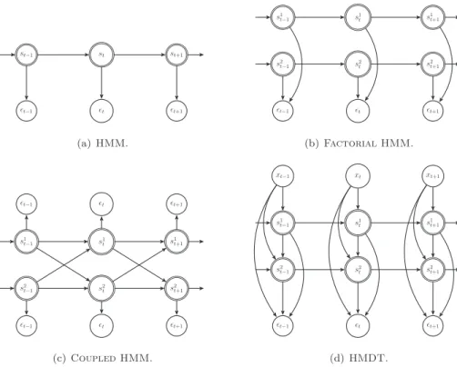
The factorial hidden Markov model (FHMM) was proposed byGhahramani and Jordan (1997). As an extension of the basic HMM, this model assumes that each state variable is factored into several state variables, each of them with its own independent Markovian dynamics, and that the output is the combination of the several processes that underlie the state variables (see figure1(b)). Because the model has various independent hidden Markov models in parallel, the resulting state space of the model is the cartesian product of the parallel sub-processes. The coupled hidden Markov model (CHMM) (seeBrand (1997)) is also an extension of the classical HMM and refers to a model with several HMMs whose Markov chains interact together (figure 1(c)).
st st−1 st+1 ǫt ǫt−1 ǫt+1 (a) HMM. s2 t s2 t−1 s 2 t+1 s1 t s1 t−1 s 1 t+1 ǫt ǫt−1 ǫt+1 (b) Factorial HMM. s2 t s2 t−1 s 2 t+1 ǫt ǫt−1 ǫt+1 s1 t s1 t−1 s 1 t+1 ǫt ǫt−1 ǫt+1 (c) Coupled HMM. s2 t s2 t−1 s 2 t+1 s1 t s1 t−1 s 1 t+1 ǫt ǫt−1 ǫt+1 xt xt−1 xt+1 (d) HMDT.
Figure 1: Hidden Markov model (1(a)), Factorial HMM (1(b)), Coupled HMM (1(c)) and Hidden Markov Decision Tree (1(d)) as graphical models. Here, st, s1t and s2t are variables follow an hidden Markov chain, ǫt the
observations and xt an (optional) variable in input.
In this framework, an HMDT provides a factorized state space that leads to a state space de-composition by level of Markov chain. Then the constraint of a level on the following is done via a coupling transition matrix which produces the ordered hierarchy of the structure. As the links between decision states are driven with Markovian dynamics, and the switch from one level to the following one is done via a coupling transition matrix, this architecture gives a fully probabilistic decision tree.
3.2. Hidden Markov decision tree for correlations 3.2.1. Starting point
The model we propose in this paper is based on the dynamic correlation class of models introduced byEngle and Sheppard (2001)). Given yt, a K dimensional time series of length T ,
the DCC class model assumes the form:
yt|Ft−1 iid
∼ N (0, Ht) (1)
where Ft−1 refers to the information set at time t − 1. The conditional variance-covariance
matrix of returns yt is expressed as follows:
Ht= DtRtDt (2)
where Rt is a K × K constant correlation matrix. The matrix Dt is a K × K diagonal matrix
containing univariate time-varying standard deviations:
Dt= diag{h1/2i,t } (3)
for i = 1, ..., K. Getting the matrix Dtis generally referred as the so-called degarching filtering
required to construct standardized residuals expressed as:
ǫt= D−1t rt (4)
The conditional correlations are simply the expectation of the standardized residuals:
Et−1[ǫtǫ′t] = Dt−1HtD−1t = Rt (5)
Many formulations have been proposed for Rt, and we refer to Bauwens et al. (2006) and
Silvennoinen and Ter¨asvirta (2009) for recent surveys in this field of research. The model we use in this study is a special case of the dynamic correlation model which allows one to classify the variances as low-regime or regime in a first step, to set up a rule to distinguish high-correlation regimes from the low-high-correlation regimes in a second step, while in a third step it links the state of the volatilities to the state of the correlations probabilistically.
3.2.2. Hidden tree structure
As pointed out in Section 3.1, an HMDT can be viewed as a factorial and coupled HMM. Decomposition of the factorial HMM is used to divide the space of the time series into low and high conditional variances for each series, and low and high for the sequences of correlations. The transition matrix used in our model can be either static or time-varying, and can depend on either endogenous or exogenous variables1. Each time series has its own conditional variance
1
To introduce time-varying transition probabilities, one can use the specification proposed byDiebold et al.
(1994). Then, transition probabilities are assumed to follow a logistic function of an endogenous or exogenous
driven by a transition matrix. As we partition the space of the univariate conditional variance in two subspaces, low and high variance, the transition matrix for the variance of the kth time
series is of size 2 × 2 and can be expressed as follows: Pkvol= pk 11 1 − pk22 1 − pk 11 pk22 (6)
Since all univariate volatility processes have the same Markovian dynamic specification, indi-vidual transition matrices can be aggregated to constitute the first level of the decision tree. Individual HMMs are aggregated in a factorial HMM representation. The dynamic of the uni-variate volatility level can be represented in a general transition matrix Pvolby the cross product
of the transition matrices of univariate volatility models Pk vol: Pvol= K p i=1 Pivol (7)
This factorial representation allows a representation of all the dynamics of the K univariate volatilities containing 2 states with a single transition matrix of size 2K× 2K.
The same specification is used for the second level. This level discriminates between low and high correlations. Thus, the decision step is represented by a 2-by-2 transition matrix written as: Pcorr= pc 11 1 − pc22 1 − pc 11 pc22 (8)
whose elements can be both static and time-varying. Given the transition matrices of the first and the second levels, the partition of the space is represented by transition matrix P expressed as:
P = Pvol⊗ Pcorr (9)
of size 2K+1× 2K+1.
Given this space partition the first and the second levels are then linked. This relation is fully probabilistic and attributes a weight to the decision related to the correlation given the decision of the univariate volatility. Formally, this link has been obtained with the use of a
coupling matrix, which is the 2-by-2 transition matrix of an abstract Markov chain that does not directly emit observations:
Pcoupl= c11 1 − c22 1 − c11 c22 (10)
To summarize the foregoing information on the probabilistic decision tree: the entire ordered hierarchy is based on a set of HMMs which partition the space. While the partitioning of space, as usually considered in binary tree models, is a recursive process following binary rules, our model has the sort which is static and defined a priori. The decision process occurs according to a cascade of ordered synchronous HMMs. The coupling process lacks the Markovian property, but can be treated as a vector of probabilities whose sum is equal to unity. By establishing a link between the HMMs, the coupling process captures the inter-process influences.
3.2.3. Specification for volatilities and correlations
In our decision tree, the first level distinguishes between low and high volatility. Thus, this decision step parameterizes a univariate regime-switching GARCH model (within the litera-ture on time series, many specifications have been proposed, e.g. Hamilton and Susmel (1994), Gray (1996),Dueker (1997),Klaassen (2002), andHaas et al. (2004)). The second level discrim-inates between low and high conditional correlations and therefore one can use a model among
those proposed in the literature (seeBillio and Caporin (2005),Pelletier (2006),Haas and Mittnik (2008)). For both volatilities or correlations there is no constraint on the choice of one specification rather
than another, and only depends on the wishes of the modeller in terms of the dynamics, parsi-mony, etc.
3.3. Estimation
Estimation of the model is done with maximum likelihood and this can be done in one or in more steps. However, as often happens in the multivariate GARCH literature, because of the high number of parameters induced by the number of series, the one step estimation remains at best challenging, if not impossible from a numerical point of view.
3.3.1. One step estimation
With the assumption of normality, the log-likelihood can be written:
L = −1 2 T Ø t=1 !K log(2π) + log(|Ht|) + yt′Ht−1yt" (11)
To be able to maximize the likelihood we need to make inferences on the state of the various Markov chains of the model. The strategy developed in our paper is to convert the complex dynamic of the factorial and coupled HMM into a simple regular HMM so that we can use standard tools for filtering and smoothing probabilities. A conversion relationship between coupled HMM and standard HMM has been proposed byBrand (1997). Given PS|S and PS′|S′
two transition matrices, PS|S′ and PS′|Stwo coupling matrices, the relationship ofBrand (1997)
is given by:
(PS|S⊗ PS′|S′).R(PS′|S⊗ PS|S′) (12)
where ⊗ denotes the Kronecker product and R is a row permute operator swapping fast and slow indices. In our case, because we use only one coupling vector in a downward direction, the regular HMM representation Preg of our model can be expressed as:
Preg= (Pvol⊗ Pcorr) ◦ (Pcoupl⊗ (ιι′)) (13)
where ◦ denotes the Hadamard product, with ι a vector of ones of length 2K+1. The conversion
into regular HMM allows us to use the standard tools for the inference of Markov chains. Let
ξjt be the probability to be in regime j given the information set available at time t − 1 and
ηjt the density under the regime j. The probability to be in each regime at time t given the
observations set up to t, written ˆξt|t, can be calculated using the following expression of the
so-called Hamilton filter:
ˆ ξt|t= ( ˆξt|t−1◦ ηt) 1′( ˆξt|t−1◦ ηt) (14) and: ˆ ξt|t+1= Preg× ˆξt|t (15)
Each state of the regular representation corresponds to a combination of possible cases, e.g. the first series in a high or a low volatility period, the second in high or low, and so on, and similarly for the correlations.
3.3.2. Multi-step estimation
Multi-step estimation is in fact composed of three steps. The parameter space θ is split into three subsets: θ1 for the parameters of the univariate volatility models, θ2 for the parameters
of the correlation model, and θ3 for the parameters of the coupling matrix. Following Engle
(2002), the log-likelihood can be written as:
L(θ1, θ2, θ3) = Lv(θ1) + Lc(θ1, θ2) + Lm(θ1, θ2, θ3) (16)
where Lv(θ1) refers to the volatility term, Lc(θ1, θ2) the correlation term, and Lm(θ1, θ2, θ3) the
coupling matrix term. Then the log-likelihood of the volatility component can be written as:
Lv(θ1) = −1 2 T Ø t=1 !K log(2π) + log(|Dt|2) + y′tD−2t yt" (17)
The correlation term is: Lv(θ1, θ2) = −1 2 T Ø t=1 !log(|Rt|) + ε′tR−1t εt− ε′tεt" (18)
and, finally, the coupling matrix term is:
Lm(θ1, θ2, θ3) = −1 2 T Ø t=1 !K log(2π) + log(|Ht|) + yt′Ht−1yt" (19)
For each step, we use Hamilton’s filter. The multi-step estimation reduces a complex estimation problem into a sequence of simple estimations. Although it seems advisable to test several initial conditions, the multi-step estimation procedure greatly reduces the time needed and the numerical complexity for the estimation of the model compared to the one-step estimation.
4. Data and empirical results
4.1. Descriptive statistics
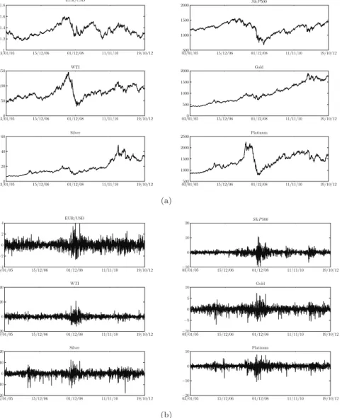
We use daily time series data (five working days per week) for WTI crude oil, euro/USD exchange rate, S&P500 index, gold, silver and platinum. All the data had been taken from the Bloomberg database2. The sample contains 1961 observations and covers the period 3 January 2005 to 19 October 2012. Thus, our dataset covers the period where the subprime crisis appeared, which is interesting for a better understanding of the dynamics and the comovement of major commodities during a financial crisis. The six series are plotted in figure 2(a). We use 100 times the difference of the logarithm of each series minus the sample mean to filter the series. The returns are plotted in figure2(b).
The main statistical features of the returns are described in table1. The daily returns have extreme maxima and minima. At the same time, each of variables has a very low mean, close to zero. Given the value of the median, variance and standard deviation, one can conclude at the presence of extreme variation of returns at certain times. All series are slightly skewed and exhibit a significant kurtosis. The Jarque-Bera test shows us that all series have fat tails with a non-normal distribution. Starting from the beginning of 2005 to 2012, our all series clearly exhibit extreme variation in the middle of the period, corresponding to the beginning of the financial crisis in August 2007. According to these basic statistics, returns of precious metals
2
The Bloomberg’s ticker for WTI is USCRWTIC, that is the West Texas Intermediate (WTI) Cushing Crude Oil Spot Price (closing price). The tickers for exchange rates and equity index are respectively EUR Curncy and SPX. For precious metals, the tickers for gold, silver and platinum are XAUUSD, XAGUSD and XPTUSD.
03/01/051 15/12/06 01/12/08 11/11/10 19/10/12 1.2 1.4 1.6 1.8 EUR/USD 03/01/05500 15/12/06 01/12/08 11/11/10 19/10/12 1000 1500 2000 S&P 500 03/01/050 15/12/06 01/12/08 11/11/10 19/10/12 50 100 150 WTI 03/01/050 15/12/06 01/12/08 11/11/10 19/10/12 500 1000 1500 2000 Gold 03/01/050 15/12/06 01/12/08 11/11/10 19/10/12 20 40 60 Silver 03/01/05500 15/12/06 01/12/08 11/11/10 19/10/12 1000 1500 2000 2500 Platinum (a) 03/01/05−4 15/12/06 01/12/08 11/11/10 19/10/12 −2 0 2 4 EUR/USD 03/01/05 15/12/06 01/12/08 11/11/10 19/10/12 −10 0 10 20 S&P 500 03/01/05 15/12/06 01/12/08 11/11/10 19/10/12 −20 0 20 40 WTI 03/01/05 15/12/06 01/12/08 11/11/10 19/10/12 −10 −5 0 5 10 Gold 03/01/05 15/12/06 01/12/08 11/11/10 19/10/12 −20 −10 0 10 20 Silver 03/01/05 15/12/06 01/12/08 11/11/10 19/10/12 −20 −10 0 10 Platinum (b)
Figure 2: Plots of EUR/USD, S&P500, WTI, Gold, Silver and Platinum series in level (subplot2(a)) and in returns (subplot2(b)).
indicate more complex dynamics, with sudden extreme variation at both the beginning and the end of the period. Engle’s LM1 test with five lags confirms the absence of serial correlation and the Engle’s DCC test strongly rejects the hypothesis of constant correlations.
4.2. Univariate volatilities
In our decision tree, the first level distinguishes between low and high volatility. Thus, this decision step parameterizes a univariate regime-switching GARCH model. In the time series
EUR/USD S&P500 WTI Gold Silver Platinum
Minimum -2.6329 -9.5798 -13.1039 -6.8348 -17.7812 -10.5209
Maximum 3.9291 10.7792 21.2380 7.3160 12.3984 7.7554
Mean 1.9061e-17 1.7984e-18 -8.4683e-17 -7.1371e-18 5.8910e-17 1.4795e-16
Median 0.0106 0.0664 0.0726 0.0382 0.1480 0.0821 Variance 0.4271 1.9407 6.3871 1.6602 5.3470 2.3769 Std deviation 0.6535 1.3931 2.5273 1.2885 2.3124 1.5417 Kurtosis 5.6800 12.3221 8.9224 6.5318 8.6123 8.4332 Skewness 0.2685 -0.2796 0.2553 -0.1754 -0.8026 -0.8287 Jarque-Bera 610.12 7122.53 2885.73 1028.75 2782.77 2635.14 KPSS∗ 0.0603 (0.1460) 0.0660(0.1460) 0.0480(0.1460) (0.1460)0.0200 (0.1460)0.0440 (0.1460)0.0648
Engle’s LM test (5 lags) 2.9535
(0.7072) 10.0055(0.0751) 6.1541(0.2915) (0.6456)3.3536 (0.9049)1.5700 10.1244(0.0718)
Engle’s DCC test (5 lags) 58.1879
(1.04e−10)
∗In brackets, critical values for the tests.
Table 1: Descriptive statistics of the returns.
literature, many specifications have been proposed. Most of them have the drawback that they require approximation schemes to avoid the path dependency problem (see Gray (1996) and Klaassen (2002)). Apart from this numerical aspect, specifications with approximations can involves difficulties in the interpretation of the processes corresponding to each regime. These considerations led us to use model ofHaas et al. (2004), which can be expressed as follows:
h1,t .. . hN,t = ω1 .. . ωN + α1 .. . αN y2t−1+ β1 .. . βN ◦ h1,t−1 .. . hN,t−1 (20)
where ◦ stands for the Hadamard product. The stationarity condition implies αn+ βn <
1 for each n = 1, ..., N . Besides its computational advantages, this approach has a clear-cut interpretation. It assumes that the conditional variance can switch between N separate (G)ARCH models that evolve in parallel. Based on the same idea, we also use a simple Markov-switching ARCH(1) model:
h1,t .. . hN,t = ω1 .. . ωN + α1 .. . αN yt−12 (21)
which is stationarity if ω > 0 and 0 < αn< 1 for each n = 1, ..., N .
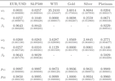
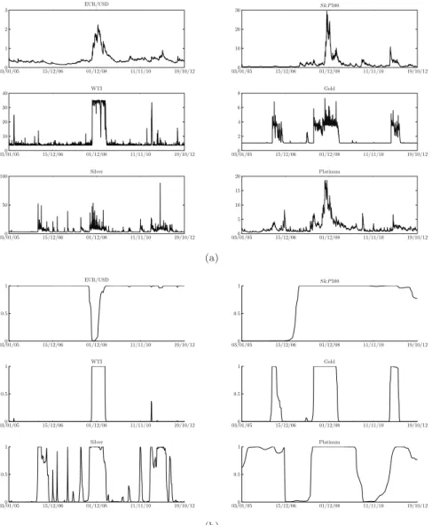
We first estimated the MS-GARCH(1,1) model for each series of returns. When this model did not give significant results, we applied the MS-ARCH(1) specification3. Both models were estimated using maximum likelihood and four random vectors of starting points. In addition to the value of the likelihood, the choice between MS-GARCH(1,1) or ARCH(1) model was conducted on the basis of the capacity of each specification to clearly identify two regimes. The total number of parameters for each series is either eight in the case of MS-GARCH(1,1) specifi-cation or six in case of MS-ARCH(1). Estimated parameters are reported in table2; estimated volatility and smoothed probabilities are plotted in figure3(a)and3(b).
EUR/USD S&P500 WTI Gold Silver Platinum
ω1 0.0031 (0.000006) (0.000044)0.0257 (21.216447)35.2410 (0.175824)3.6014 (2.327958)8.8684 (0.000217)0.0204 α1 0.0257 (0.000074) (0.000228)0.1040 (0.000017)0.0000 (0.002267)0.0698 (0.012960)0.2559 (0.000348)0.0671 β1 0.9643 (0.000209) (0.000205)0.8843 - - - (0.000541)0.9229 ω2 0.0260 (0.001190) (0.000205)0.0283 (0.029090)3.6287 (0.003588)1.0569 (0.064081)2.8845 (0.004677)0.2771 α2 0.0257 (0.005748) (0.000261)0.0310 (0.001508)0.1129 (0.001370)0.0000 (0.001502)0.0061 (0.001404)0.1446 β2 0.9643 (0.007179) (0.000646)0.9029 - - - (0.004409)0.5929 p11 0.9997 (0.000000) (0.000000)0.9997 (0.000129)0.9873 (0.000019)0.9936 (0.000073)0.9831 (0.000001)0.9989 p22 0.9850 (0.000150) (0.000001)0.9995 (0.000000)0.9999 (0.000000)1.0000 (0.000017)0.9934 (0.000009)0.9960
Table 2: Estimated parameters for Markov-switching ARCH(1) and GARCH(1,1) models. The standard errors are in brackets.
The results of the model specification appear to be quite clear-cut. The volatility of the ex-change rates, S&P500 index, and platinum was successfully modelled by the MS GARCH(1,1) specification, whereas the volatility of oil, gold, and silver was better modelled by the parsimo-nious MS ARCH(1) specification. By definition, the difference between the two models was that
3
The choice between MS-ARCH or MS-GARCH was not done using standard information criterions as AIC or BIC. As we must discriminate between two regimes, the selection was done by the ability of the model to correctly identify two regimes, with an order of preference from MS-GARCH to MS-ARCH.
03/01/050 15/12/06 01/12/08 11/11/10 19/10/12 1 2 3 EUR/USD 03/01/050 15/12/06 01/12/08 11/11/10 19/10/12 10 20 30 S&P 500 03/01/050 15/12/06 01/12/08 11/11/10 19/10/12 10 20 30 40 WTI 03/01/050 15/12/06 01/12/08 11/11/10 19/10/12 2 4 6 8 Gold 03/01/050 15/12/06 01/12/08 11/11/10 19/10/12 50 100 Silver 03/01/050 15/12/06 01/12/08 11/11/10 19/10/12 5 10 15 20 Platinum (a) 03/01/050 15/12/06 01/12/08 11/11/10 19/10/12 0.5 1 EUR/USD 03/01/050 15/12/06 01/12/08 11/11/10 19/10/12 0.5 1 S&P 500 03/01/050 15/12/06 01/12/08 11/11/10 19/10/12 0.5 1 WTI 03/01/050 15/12/06 01/12/08 11/11/10 19/10/12 0.5 1 Gold 03/01/050 15/12/06 01/12/08 11/11/10 19/10/12 0.5 1 Silver 03/01/050 15/12/06 01/12/08 11/11/10 19/10/12 0.5 1 Platinum (b)
Figure 3: Estimated univariate volatilities (subplot 3(a)) and smoothed probabilities (subplot3(b)).
the GARCH has a conditional variance that is a linear function of the lagged squared values of the series and those of its own lags. In our case, the problem arose with the estimation of the parameter β, associated with the lagged variance. Typically, when applying MS-GARCH(1,1) for oil, gold, and silver, the estimated value of the parameter β is close to 0.9 in one regime and 0.4 in the other regime. This means that it is difficult to represent the turbulent period with a GARCH model due to the extreme variations that might occur during a short period. When
the parameter β is near to unity, the impact of a shock on volatility appeared to be a persistent phenomenon. In the case where β is equal to zero (the ARCH model), the volatility can have a very sharp response to shocks. We can conclude from the foregoing that the volatility of oil, gold, and silver responded strongly to shocks, while shocks had a more persistent, lingering effect on the volatility of the exchange rate, S&P500, and platinum.
Another finding thrown up by the first level of our analysis relates to the periods during which changes in a regime occur. This information is provided by the smoothed probabilities. Hereafter, and for the sake of simplicity, we shall consider a variable to be in a given regime when the smoothed probability is at least equal to 0.99. We shall also refer to the regime as-sociated with low volatility as regime 1, and to the regime asas-sociated with turbulent volatility as regime 2. One can distinguish the three groups given the dating of the smoothed probabilities.
The first group included exchange rates and oil. For the exchange rates, the dating of the change in regime is very clear. The exchange rate started to fall into regime 2 on 9th July 2008. This occurrence is clear but relatively short, since the regime ended on 23rd September 2008 with the probability of being in regime 1 equal to 0.999. This result accords well with the timing of the exchange rate fluctuation. The value of one euro was 1.6038 US dollar on 15th July 2008, a value that was the currency’s maximum for the year, but it suffered a considerable fall on 24th October the same year to 1.2530 US dollar. Thus regime 2 of the exchange rate was characterized by two attributes: a globally high value (the constant ω in the GARCH process larger in regime 2 than in regime 1 by a factor of 10), and very high volatility. The timing was about the same in the case of oil, regime 2 arriving on 18th September 2008, and ending on 6th May 2009. As has been said before, the volatility of oil is best taken into account by an MS-ARCH(1,1) model. Once again, regime 2 showed a high volatility component with variation ranging from 120.92 USD on 19th September 2008 to 31.41 USD on 19th December 2008. The second group had only one series, namely the S&P500, and the dynamic of its volatility was comparatively simple. The index tumbled into regime 2 around 5th September 2007, and remained there until the end of the period. During regime 2, the stock market index rose to its maximum on 8th October 2007 at 1565.2, and dropped to its minimum at 676.03 on 6th March 2009.
The third group consisted of precious metals. The smoothed probabilities lent support to the notion of clubbing the metals into a single group, given their similar volatility patterns. Now,
while the three precious metals exhibited three phases of regime 2 in their responses to shocks, the durations of these responses varied considerably. The chart of the smoothed probabilities shows the onset of the first appearance of regime 2 with one month’s gap between gold (15th May 2006) and silver (19th April 2006). However, the duration of that phase of regime 2 is shorter in the case of gold than it is in the case of silver, ending respectively on 23rd October 2006 and 20th October 2006. In the case of platinum, the phase ended in late November. The second phase of regime 2 appeared during the Subprime crash, its timing varying with the specific metal. The turbulent period began on 18th March 2008 for gold, 29th August 2008 for silver, and 29th February 2008 for platinum. That period ended on 4th May 2009 for gold, 22nd June 2009 for silver, and 4th June 2010 for platinum. Clearly, platinum remained longer in regime 2 than did the other two metals. We observed a strong upward movement in precious metals with a delayed effect for silver and platinum in comparison with gold. Regime 2 appeared on 23rd August 2011 for gold, on 14th September 2011 for silver, and 28th October 2011 for platinum. As in the previous case, we observed that resistance to shocks was lower in the case of gold than it was in the case of the other two metals. The third phase of regime 2 ended on 12th January 2012 for gold, in late February 2012 for silver, and showed no end in the case of platinum. To sum up our results for the period under review, gold and silver showed themselves to be very reactive to economic shocks, while platinum responded slowly.
4.3. Correlations
The specification used for the correlation was that ofPelletier (2006), who proposes a Markov-switching structure for the correlation process by imposing constant correlations in each regime and establishing the switch of each other through a Markov chain of order one. Called Regime Switching for Dynamic Correlation (RSDC), the choice of the RSDC model was motivated by the idea of having an easily interpretable model from an economic point of view. Formally, the RSDC model assumes that the conditional correlation matrix Rt has the following form:
Rt= N
Ø
n=1
1{sn=i}Rn (22)
where {st}t∈N is a sequence of a homogeneous first order Markov chain with N states. Rn
is a conditional correlation matrix of size K × K where Rn Ó= Rn′ for n Ó= n′. In our
anal-ysis, we use two regimes that refer respectively to constant correlation matrices R1 and R2.
The model has been estimated using maximum likelihood and four random vectors of starting points. Standardised residuals have been computed given the de-garching filtering of the last
03/01/05 01/12/08 19/10/12 −0.0139
0.4645
EUR/USD and S&P 500
03/01/05 01/12/08 19/10/12 0.2256
0.4587
EUR/USD and WTI
03/01/05 01/12/08 19/10/12 0.3567
0.5115
EUR/USD and Gold
03/01/05 01/12/08 19/10/12 0.4359
0.4962
EUR/USD and Silver
03/01/05 01/12/08 19/10/12 0.3611
0.4544
EUR/USD and Platinum
03/01/05 01/12/08 19/10/12 0.0189
0.5738 S&P 500 and WTI
03/01/05 01/12/08 19/10/12 0.0161
0.1533 S&P 500 and Gold
03/01/05 01/12/08 19/10/12 0.0896
0.3065 S&P 500 and Silver
03/01/05 01/12/08 19/10/12 0.0652
0.3614 S&P 500 and Platinum
03/01/05 01/12/08 19/10/12 0.307
0.3368
WTI and Gold
03/01/05 01/12/08 19/10/12 0.3559
0.4117 WTI and Silver
03/01/05 01/12/08 19/10/12 0.2624
0.4445 WTI and Platinum
03/01/05 01/12/08 19/10/12 0.805
0.8264
Gold and Silver
03/01/05 01/12/08 19/10/12 0.5873
0.7162 Gold and Platinum
03/01/05 01/12/08 19/10/12 0.5835
0.7407 Silver and Platinum
Figure 4: Estimated correlations.
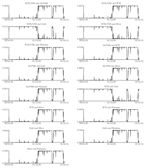
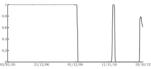
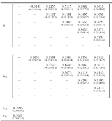
paragraph. Estimated parameters are reported in table3; estimated correlations and smoothed probabilities are plotted in figures4and 5.
The first result of the correlation level is about the dating of the regimes. The sample begins in non-crisis regime up to the end of January 2009. In our analysis, the break in the correlations occurs just after the last quarter of 2008 which is considered as the peak of the Subprime crisis. It is interesting to note that, for correlations, regime 2 began almost just when it was ending for the volatility of the univariate series of the exchange rates, oil prices, and the prices of gold
03/01/050 15/12/06 01/12/08 11/11/10 19/10/12 0.2 0.4 0.6 0.8 1
Figure 5: Smoothed probability for RSDC.
and silver. There was a short interval between these occurrences of regime 2 depending on whether the analysis was conducted at a univariate level or at a multivariate level. Therefore, while all the variables had their own timing for correlations, which sometimes differed from the chronology of the Subprime crisis, the break in the correlations coincided exactly with the crash that came at the end of 2008. The correlation dynamics also experienced a break from the middle of March 2011 to the end of that month, more precisely, from 14th March 2011 to 28th March 2011. One might assume that the shock behind that break was Tohoku earthquake of 2011, and the tsunami which resulted which caused massive damage to Japan’s economy. The effect of that happening is reflected in our series, but it might be interpreted as a statistical artifact. Equally interesting would be the thought that the tsunami might not have induced the break at the univariate level of analysis, but that it did have an effect at the multivariate level. The second result concerns the level of the correlations. Our results clearly point to the distinction between two main types of econometric relation: correlations that are quasi-constant or constant in time throughout the period under study, and correlations that increase while switching from regime 1 to regime 2. We only had a single correlation outside of these two main groups, which showed a significant decrease when switching from regime 1 to regime 2. The first type of relation implies stability across time, in times of crisis as in normal times. The correlation value in our study did not remain unchanged between the two regimes, but the variation was too marginal to be considered significant. That was the case for the correlations between oil and gold (0.33 to 0.30) and silver (0.35 to 0.41). It was not surprising that the correlations of gold and silver were constant during the sample period (0.80 to 0.82). This finding tended to confirm that the two precious metals move together on the commodities market. It was more difficult to explain the steady correlation between silver and the exchange rates (0.49 to 0.43). The second group showed the behaviour one encounters in the literature on econometrics, namely, an increase in the correlation for platinum and gold and silver remained steady: an increase of 0.13 for gold, and 0.16 for silver. It is also notable that platinum was highly correlated in regime
R1 − −0.0141 (0.003208) (0.000686)0.2255 (0.010841)0.5115 (0.002678)0.4962 (0.008185)0.3611 − − 0.0187 (0.001170) (0.001133)0.0161 (0.000497)0.0895 (0.001355)0.0651 − − − 0.3368 (0.000650) (0.000252)0.3558 (0.000417)0.2623 − − − − 0.8050 (0.000119) (0.001130)0.5873 − − − − − 0.5834 (0.000345) − − − − − − R2 − 0.4654 (0.019994) (0.113053)0.4591 (0.176734)0.3564 (0.144050)0.4358 (0.091147)0.4546 − − 0.5749 (0.016382) (0.068160)0.1536 (0.022561)0.3069 (0.117005)0.3619 − − − 0.3070 (0.100540) (0.034904)0.4118 (0.053340)0.4449 − − − − 0.8264 (0.000271) (0.010190)0.7165 − − − − − 0.7410 (0.003235) − − − − − − p11 0.9996 (0.000000) p22 0.9981 (0.000021)
Table 3: Estimated parameters correlation model RSDC. The standard errors are in brackets. The order of the columns (and rows) is as follows: exchange rate, S&P500, oil, gold, silver and platinum.
1 with gold and silver, with a value of 0.58 for both the metals. One would thus have two subsets in this group: gold and silver in one subset, and platinum in the other. Oil showed an increase in the correlation with macroeconomic variables, S&P500 (0.01 to 0.57) and exchange rates (0.22 to 0.45). Platinum was the only precious metal on which oil showed an increased dependence (0.26 to 0.44). The upward variations of S&P500 correlations with gold and silver were very close (0.01 to 0.15 and 0.08 to 0.30) respectively. The third group represents correlations which decreased between regime 1 and regime 2. There was only one pair of correlations, between gold and the exchange rate, which fell (from 0.51 to 0.35). The decrease of EURO/USD is consistent with those ofCiner et al. (2013) who argue that gold can act a safe haven against exchange rate movements.
4.4. The link between volatilities and correlations
The estimated results of the coupling transition matrix define the relationship between the first and the second levels, that is, the linkages between the univariate volatilities and the
correlations. We used a coupling transition matrix, with one given regime of volatility associated with each regime of correlation. From the previous results, this vertical relation needed only a single 2-by-2 coupling matrix for estimation. The model was estimated using maximum likelihood and four random vectors as starting points. The smoothed probabilities for a variable to be in regime 1 for correlations given that the univariate volatilities are in low or turbulent regime are plotted in figure6and estimated parameters are in table 4.
The first results are related to all series. Given regime 1 or regime 2 of volatility, what is the
03/01/050 15/12/06 01/12/08 11/11/10 19/10/12 0.2 0.4 0.6 0.8 1 Low volatility 03/01/050 15/12/06 01/12/08 11/11/10 19/10/12 0.2 0.4 0.6 0.8 1 Turbulent volatility
(a) All series
03/01/050 15/12/06 01/12/08 11/11/10 19/10/12 0.2 0.4 0.6 0.8 1 Low volatility 03/01/050 15/12/06 01/12/08 11/11/10 19/10/12 0.2 0.4 0.6 0.8 1 Turbulent volatility (b) Metals only 03/01/050 15/12/06 01/12/08 11/11/10 19/10/12 0.2 0.4 0.6 0.8 1 Low volatility 03/01/050 15/12/06 01/12/08 11/11/10 19/10/12 0.2 0.4 0.6 0.8 1 Turbulent volatility
(c) Oil and gold
03/01/050 15/12/06 01/12/08 11/11/10 19/10/12 0.2 0.4 0.6 0.8 1 Low volatility 03/01/050 15/12/06 01/12/08 11/11/10 19/10/12 0.2 0.4 0.6 0.8 1 Turbulent volatility
(d) EUR/USD, S&P500 and WTI
Figure 6: Smoothed probabilities to be in regime 1 for correlations given univariate volatilites are in low or turbulent regime.
probability of the variable being in regime 1 or regime 2 in the correlations? The smoothed probabilities of being in regime 1 of volatilities in a bear market, given low volatility (regime 1 of volatilities) and the smoothed probabilities of variable being in regime 1 of correlations in a bull market given the volatilities are turbulent are presented in sub-plot6(a). Low volatilities were clearly associated with low correlations up to the beginning of the year 2000. Thereafter the probability of regime 2 of correlations given low volatility was zero Turbulent volatilities are not associated in bull market correlations. From the beginning of the period to early 2009, the regime of turbulent volatilities was clearly linked to regime 1 of correlations (low level of correlations). The switch appeared with the Subprime crisis and the Tohoku earthquake. The results highlight dynamics with a succession of switches between regime 1 and regime 2 of
correlations when precious metals had low volatility (figure6(b)). This might mean that such metals have a very specific behaviour when the volatilities are low, and their correlations can switch from one state to the other independently of the prevailing economic trends. On the other hand, turbulent regimes in volatility are directly associated with regime 2 of volatility with a probability of one across the entire period. Put another way, high variations in the volatility of precious metals cause them to behave the same way.
The relationship of the volatility of oil and gold and the correlations could not be clearer. The case of low volatility is associated throughout the entire sample period with the low-correlation regimes. The state of turbulent volatility is linked to high-correlation regimes (figure6(c)).
The link between the exchange rates, S&P500, and WTI was not identified when all the series
All series Metals only Oil and gold EUR/USD, S&P500 and WTI
Low volatility p11 1.0000 (0.000000) (0.000299)0.9488 (0.000729)1.0000 (0.000000)0.0000 p22 1.0000 (0.000000) (0.000047)0.9884 (0.000000)0.0000 (0.002712)0.8450 High volatility p11 1.0000 (0.000000) (0.021182)1.0000 (0.000000)0.0000 (0.000000)0.9995 p22 0.9986 (0.000002) (0.000305)0.0000 (0.050136)1.0000 (0.000016)0.9966
Table 4: Estimated parameters for transition matrix linking the volatility and the correlations. The standard errors are in brackets.
had low volatilities. In the cases of turbulent volatilities, the probability of regime 1 for the correlation was equal to one from the beginning of the sample period to early 2009. This was also the case for the period covering the Tohoku earthquake (figure6(d)).
5. Conclusion
We have studied the relationship between univariate volatilities and correlations among euro/US dollar exchange rate, S&P500, WTI crude oil, and three major precious metals, namely gold, silver and platinum, over the period 3 January 2005 to 19 October 2012. The contributions of our paper are of twofolds: methodological and empirical.
Results were obtained using a model based on the Hidden Markov Decision Tree (HMDT). In-troduced byJordan et al. (1997), HMDT is in fact an extension of the Hidden Markov Model (HMM) and is the opposite of the classical deterministic approach based on a binary decision
tree. This specification allows one to quantify probabilistically the relationship inside a par-titioned space. The model is fully probabilistic. The tree used in this paper has two levels: the first discriminates between low and turbulent volatilities, the second between low and high correlations. At each level, the classification was carried out with a Markov-switching model. The two levels were then linked such that one would have the probability to be in a regime of correlation given the regime of volatilities. As far as we know, unlike deterministic binary tree models, stochastic tree specifications have not been used up until now in the study of the linkages beween volatilities and correlations.
The empirical results highlight several elements of the dynamic of our dataset. First, we found that the volatility of oil, gold, and silver responded strongly to shocks. Shocks had a more per-sistent effect on the volatility of the exchange rates, S&P500 indices, and platinum prices. The exchange rates, and oil plunged into the turbulent volatility regime at the peak of the Subprime crisis in the fall of 2008 to the spring of 2009. The S&P500 switched into the turbulent regime in the fall of 2007, and remained there until the end of the sample. Precious metals showed nearly the same dynamics with three periods in the turbulent regimes. While all precious metals were sensitive to the same shocks, the lengths of their reaction were not the same. Secondly, our model showed that the correlations slipped into regime 2 just after the last quarter of 2008, coin-ciding with the Subprime crisis. The correlations switched a second time, though briefly, during the Tohoku earthquake. Third, the vertical probabilities highlight the relationship between the volatilities and the correlations. We found that low volatilities were associated with low corre-lations from the beginning of the period to the early 2009. The conclusion was the same with a turbulent regime of volatilities, that was linked to a low regime of correlations, which again was linked to a probability of one with low correlations during the first half the period and the Tohoku earthquake. In the case of precious metals, turbulent volatilities were clearly linked to the rise of the correlations. How precisely the low volatility regime of precious metals is linked to the state of the correlations, would requiel a somewhat lengthy and complicated explanation of the phenomenon. The results for gold and oil threw up one of the most surprising findings of our study, specifically that a low-volatility regime had a probability of one of being associated with high correlations throughout the sample period. The turbulent-volatility regime is itself linked to low correlations. However, our model was unable to identify the relation between the correlation regimes and low volatility in the case of the group consisting of the exchange rates, the equity indices, and the oil prices. Nevertheless, the model provided an indication that turbulent-volatility regimes were linked to low-volatility regimes during the first half of the
sample period and particularly after the Japanese earthquake. Our results tend to contradict the findings of previous studies, specifically that correlations increase in bear markets, e.g. Ang and Chen (2002), Longin and Solnik (2001), and Campbell et al. (2002), all of which had fo-cused their attention on international equity returns or indices. A contradiction such as this could be a result of the choice of the series and the sample period. Our sample consisted of two macroeconomic variables and four commodities. Our results showed that within the group of commodities studied, oil and precious metals possessed their own distinct dynamics, and showed their own type of response to shocks.
The model developed in this paper could prove to be a useful tool with which to deepen our understanding of volatility and correlation. The specification that we used remains very simple, with only two levels and without introducing exogenous variables. It could be interesting to build complex Markovian tree-based structures to understand the determinant of correlations.
References
Adrangi, B., Chatrath, A., April 2002. The dynamics of palladium and platinum prices. Com-putational Economics 19 (2), 179–95.
Agnolucci, P., March 2009. Volatility in crude oil futures: A comparison of the predictive ability of garch and implied volatility models. Energy Economics 31 (2), 316–321.
Akgiray, V., Booth, G., Hatem, J., C., M., August 1991. Conditional dependence in precious metal prices. The Financial Review 26 (3), 367–86.
Ang, A., Bekaert, G., 2002. International asset allocation with regime shifts. Review of Financial Studies 15 (4), 1137–1187.
Ang, A., Chen, J., 2002. Asymmetric correlations of equity portfolios. Journal of Financial Economics 63 (3), 443–494.
Arouri, M. E. H., Hammoudeh, S., Lahiani, A., Nguyen, D. K., 2012. Long memory and struc-tural breaks in modeling the return and volatility dynamics of precious metals. The Quarterly Review of Economics and Finance 52 (2), 207–218.
Baffes, J., September 2007. Oil spills on other commodities. Resources Policy 32 (3), 126–134. Batten, J. A., Ciner, C., Lucey, B. M., June 2010. The macroeconomic determinants of volatility
Bauwens, L., Laurent, S., Rombouts, J., 2006. Multivariate garch models : a survey. Journal of Applied Econometrics 21 (1), 79–109.
Billio, M., Caporin, M., 2005. Multivariate markov switching dynamic conditional correlation garch representations for contagion analysis. Statistical Methods and Applications 14 (2), 145–161.
Bollerslev, T., 1986. Generalized autoregressive conditional heteroskedasticity. Journal of Econo-metrics 31 (3), 307–327.
Brand, M., 1997. Coupled hidden markov models for modeling interacting processes. Technical report 405, MIT Media Lab Perceptual Computing.
Cai, J., Cheung, Y.-L., Wong, M. C. S., 2001. What moves the gold market? Journal of Futures Markets 21, 257–278.
Campbell, R., Koedijk, K., Kofman, P., 2002. Increased correlation in bear markets. Financial Analysts Journal 58 (1), 87–94.
Cashin, P., McDermott, C. J., Scott, A., Dec. 1999. The myth of co-moving commodity prices. Reserve bank of new zealand discussion paper series, Reserve Bank of New Zealand.
Chen, M.-H., September 2010. Understanding world metals prices–returns, volatility and diver-sification. Resources Policy 35 (3), 127–140.
Cheong, C. W., June 2009. Modeling and forecasting crude oil markets using arch-type models. Energy Policy 37 (6), 2346–2355.
Cheung, Y.-W., Lai, K. S., May 1993. Do gold market returns have long memory? The Financial Review 28 (2), 181–202.
Christie-David, R., Chaudhry, M., Koch, T. W., 2000. Do macroeconomics news releases affect gold and silver prices? Journal of Economics and Business 52 (5), 405–421.
Ciner, C., 2001. On the long run relationship between gold and silver prices: A note. Global Finance Journal 12, 299–303.
Ciner, C., Gurdgiev, C., Lucey, B. M., 2013. Hedges and safe havens: An examination of stocks, bonds, gold, oil and exchange rates. International Review of Financial Analysis 29 (0), 202 – 211.
Cochran, S. J., Mansur, I., Odusami, B., 2012. Volatility persistence in metal returns: A figarch approach. Journal of Economics and Business 64 (4), 287–305.
Coudert, V., Mignon, V., Penot, A., 2007. Oil price and the dollar. Energy Studies Review 15 (2).
Deb, P., Trivedi, P. K., Varangis, P., May-June 1996. The excess co-movement of commodity prices reconsidered. Journal of Applied Econometrics 11 (3), 275–91.
Diebold, F., Lee, J., Weinbach, G., 1994. Regime switching with time-varying transition prob-abilities. In: Hargreaves, C. (Ed.), Non-Stationary Time Series Analysis and Co-Integration, advanced texts in econometrics Edition. The Clarendon Press & Oxford University Press. Diebold, F. X., Inoue, A., November 2001. Long memory and regime switching. Journal of
Econometrics 105 (1), 131–159.
Dueker, M. J., 1997. Markov switching in garch processes and mean-reverting stock-market volatility. Journal of Business & Economic Statistics 15 (1), 26–34.
Elder, J., Miao, H., Ramchander, S., 2012. Impact of macroeconomic news on metal futures. Journal of Banking & Finance 36 (1), 51–65.
Engle, R., 2002. Dynamic conditional correlation - a simple class of multivariate garch models. Journal of Business and Economic Statistics 20, 339–350.
Engle, R., Sheppard, K., 2001. Theoretical and empirical properties of dynamic conditional correlation multivariate garch. Working Paper 2001–15, UCSD.
Engle, R. F., 1982. Autoregressive conditional heteroscedasticity with estimates of the variance of united kingdom inflation. Econometrica 50 (4), 987–1007.
Escribano, A., Granger, C., 1998. Investigating the relationship between gold and silver prices. Journal of forecasting 17, 81–107.
Ghahramani, Z., Jordan, M. I., 1997. Factorial hidden Markov models. Machine Learning 29, 245–273.
Granger, C. W. J., Hyung, N., June 2004. Occasional structural breaks and long memory with an application to the s&p 500 absolute stock returns. Journal of Empirical Finance 11 (3), 399–421.
Gray, S., 1996. Modeling the conditional distribution of interest rates as a regime-switching process. Journal of Financial Economics 42, 27–62.
Haas, M., Mittnik, S., 2008. Multivariate regime-switching garch with an application to inter-national stock markets. CFS Working Paper Series 2008-08, Center for Financial Studies. Haas, M., Mittnik, S., Paollela, M., 2004. A new approach to markov-switching garch models.
Journal of Financial Econometrics 2 (4), 493–530.
Hamilton, J., Susmel, R., 1994. Autoregressive conditional heteroskedasticity and change in regime. Journal of Econometrics 64, 307–333.
Hamilton, J. D., 2009. Causes and consequences of the oil shock of 2007-08. Brookings Papers on Economic Activity 40 (1 (Spring)), 215–283.
Hess, D., Huang, H., Niessen, A., 2008. How do commodity futures response to macroeconomic news? Financial Markets and Portfolio Management 22, 127–146.
Hong, Y., Tu, J., Zhou, G., 2007 23 2006. Asymmetries in stock returns: Statistical tests and economic evaluation. Review of Financial Studies 20 (5), 1547–1581.
Jordan, M., Ghahramani, F., Saul, L., 1997. Hidden markov decision trees. In: Mozer, M. C., Jordan, M. I., Petsche, T. (Eds.), Advances in Neural Information Processing Systems (NIPS) 9. Cambridge MA: MIT Press.
Kang, S. H., Kang, S.-M., Yoon, S.-M., January 2009. Forecasting volatility of crude oil markets. Energy Economics 31 (1), 119–125.
Klaassen, F., 2002. Improving garch volatility forecasts with regime-switching garch. Empirical Economics 27 (2), 363–394.
Krugman, P. R., Jun. 1983a. Oil and the dollar. Nber working papers, National Bureau of Economic Research, Inc.
Krugman, P. R., 1983b. Oil shocks and exchange rate dynamics. In: Exchange Rates and Inter-national Macroeconomics. National Bureau of Economic Research, Inc, pp. 259–284.
Longin, F., Solnik, B., 1995. Is the correlation in international equity returns constant : 1960– 1990 ? Journal of International Money and Finance 14 (1), 3–26.
Longin, F., Solnik, B., 2001. Extreme correlation of international equity markets. Journal of Finance 56, 651–678.
Lucey, B. M., Tully, E., January 2006a. The evolving relationship between gold and silver 1978– 2002: evidence from a dynamic cointegration analysis: a note. Applied Financial Economics Letters 2 (1), 47–53.
Lucey, B. M., Tully, E., 2006b. Seasonality, risk and return in daily comex gold and silver data 1982-2002. Applied Financial Economics 16 (4), 319–333.
Lunde, A., Hansen, P. R., 2005. A forecast comparison of volatility models: does anything beat a garch(1,1)? Journal of Applied Econometrics 20 (7), 873–889.
Nomikos, N. K., Pouliasis, P. K., March 2011. Forecasting petroleum futures markets volatility: The role of regimes and market conditions. Energy Economics 33 (2), 321–337.
Pelletier, D., 2006. Regime switching for dynamic correlations. Journal of Econometrics 131 (1– 2), 445–473.
Pindyck, R. S., Rotemberg, J. J., December 1990. The excess co-movement of commodity prices. Economic Journal 100 (403), 1173–89.
Plourde, A., Watkins, G. C., September 1998. Crude oil prices between 1985 and 1994: how volatile in relation to other commodities? Resource and Energy Economics 20 (3), 245–262. Roache, S. K., Rossi, M., 2010. The effects of economic news on commodity prices. The Quarterly
Review of Economics and Finance 50 (3), 377–385.
Sari, R., Hammoudeh, S., Soytas, U., March 2010. Dynamics of oil price, precious metal prices, and exchange rate. Energy Economics 32 (2), 351–362.
Schwartz, E. S., July 1997. The stochastic behavior of commodity prices: Implications for valuation and hedging. Journal of Finance 52 (3), 923–73.
Silvennoinen, A., Ter¨asvirta, T., 2009. Multivariate garch models. In: Andersen, T., Davis, R., Kreiss, J., Mikosch, T. (Eds.), Handbook of Financial Time Series. Springer, New York.
Sjaastad, L. A., June 2008. The price of gold and the exchange rates: Once again. Resources Policy 33 (2), 118–124.
Sjaastad, L. A., Scacciavillani, F., December 1996. The price of gold and the exchange rate. Journal of International Money and Finance 15 (6), 879–897.
Throop, A. W., 1993. A generalized uncovered interest parity model of exchange rates. Economic Review, 3–16.
van Amano, R. A., Norden, S., November 1998. Exchange rates and oil prices. Review of Inter-national Economics 6 (4), 683–94.
Wang, Y., Wu, C., 2012. Forecasting energy market volatility using garch models: Can multi-variate models beat unimulti-variate models? Energy Economics 34 (6), 2167–2181.
Zhang, Y.-J., Wei, Y.-M., September 2010. The crude oil market and the gold market: Evidence for cointegration, causality and price discovery. Resources Policy 35 (3), 168–177.
Les Cahiers de la Chaire Finance rassemblent les documents de travail du LEMNA s'inscrivant dans des projets de recherche qu'elle soutient.
N° 2012-06
Are Islamic Indexes more Volatile than Conventional Indexes?
Evidence from Dow Jones Indexes
CHARLES Amélie, DARNÉ Olivier et POP Adrian
N° 2012-07
Large Shocks in the Volatility of the Dow Jones Industrial Average
Index: 1928-2010
CHARLES Amélie et DARNÉ Olivier
N° 2012-08
The Quality of Private Monitoring in European Banking: Completing
the Picture
POP Adrian et POP Diana
N° 2012-09
Effets socioéconomiques de la crise financière : implications pour le
Vietnam
LAUZANAS Jean-Marc, PERRAUDEAU Yves et POP Adrian
N° 2012-31
Efficiency Gains from Narrowing Banks: A Search-Theoretic Approach
TRIPIER Fabien
N° 2012-32
Volatility Persistence in Crude Oil Markets
CHARLES Amélie et DARNÉ Olivier
N° 2012-40
La modélisation en équilibre général et stochastique des cycles
économiques en Afrique Sub-saharienne : une revue de la littérature
NOUASSI Claude Francis et TRIPIER Fabien
Les opinions exposées dans ce document n’engagent que les auteurs. Ceux-ci assument la responsabilité de toute erreur ou omission.
La Chaire Finance est une initiative de la Banque Populaire Atlantique, la Caisse d’Epargne Bretagne-Pays de Loire, la Caisse des Dépôts, du Crédit Maritime et de l’Université de Nantes, sous l’égide de la Fondation de Projets de l’Université de Nantes.
Site web : http://www.univ-nantes.fr/fondation/chairefinance
Contact
Chaire Finance, Banque Populaire – Caisse d’Epargne IEMN-IAE, Chemin de Censive du Tertre – BP 52231
44322 Nantes cedex 3 Tél : +33 (0)2 40 14 16 60 Fax : +33 (0)2 40 14 16 50