Distributed construction of energy-efficient ad hoc wireless broadcast trees

Distributed Construction of Energy-Efficient Ad Hoc

Wireless Broadcast Trees

by

Ashwinder S. Ahluwalia

Submitted to the Department of Electrical Engineering and Computer

Science

in partial fulfillment of the requirements for the degree of

Master of Engineering in Computer Science and Engineering

at the

MASSACHUSETTS INSTITUTE OF TECHNOLOGY

Feb 2002

© Ashwinder S. Ahluwalia, MMII. All rights reserved.

The author hereby grants to MIT permission to reproduce and distribute

publicly paper and electronic copies of this thesis document in whole or in

part.

Author ...

17"" ..••••••••••••••••••••••••••.•••••••••••••••••••••••••••

Department of Electrical Engineering and Computer Science

Feb. 1,2002

Certified by ...

7 ' ... -...

< • • • • • • • • • • • •

E~~·

M~di;';'~

Assistant Professor, Department of Aeronautics and Astronautics

Thesis Supervisor

Certified by ...

T . . . .

Dr. Li Shu

Communications and Network Engineer, The Charles Stark Draper

Laboratory

Thesis Supervisor

Accepted by ... .

Arthur C. Smith

Chairman, Department Committee on Graduate Students

Distributed Construction of Energy-Efficient Ad Hoc Wireless

Broadcast Trees

by

Ashwinder S. Ahluwalia

Submitted to the Department of Electrical Engineering and Computer Science on Feb. 1, 2002, in partial fulfillment of the

requirements for the degree of

Master of Engineering in Computer Science and Engineering

Abstract

We address the energy-efficient broadcasting problem in ad hoc wireless networks. First we show that finding the minimum energy broadcast tree is NP-complete and develop an approximation algorithm, which computes sub-optimal solutions in polynomial time. We present a distributed algorithm that computes all N possible broadcast trees simultaneously with

O(N2 )

message complexity. We compare our algorithm's performance to the best known centralized algorithm, and show that it constructs trees consuming, on average, only 18% more energy. Finally, we introduce the multiple source broadcasting problem, and explore algorithms that address this problem.

Thesis Supervisor: Eytan Modiano

Title: Assistant Professor, Department of Aeronautics and Astronautics

Thesis Supervisor: Dr. Li Shu

Acknowledgment 2/1/02

This thesis was prepared at The Charles Stark Draper Laboratory, Inc., under IR&D, GCC group, charge

#

18542.

Publication of this thesis does not constitute approval by Draper or the sponsoring agency of the findings or conclusions contained herein. It is published for the exchange and stimulation of ideas.

Assignment

Draper Laboratory Report Number T -1420

In consideration for the research opportunity and permission to prepare my thesis by and at The Charles Stark Draper Laboratory, Inc., I hereby assign my copyright of the thesis to The Charles Stark Draper Laboratory, Inc., Cambridge, Massachusetts.

!J1tb.

(author's signature)

~{'/o,­

Contents

1 Introduction 1.1 Problem Formulation 1.2 Background . . . . 1.2.1 Complexity 1.2.2 Algorithms

1.2.3 The need for a distributed algorithm

2 Complexity

2.1 Relevant Background Work 2.2 Proof of NP-completeness .

3 Constructing Broadcast Trees

3.1 The Broadcast Incremental Protocol (BIP) 3.1.1 Improving BIP: Hybrid Algorithms 3.2 Computing Broadcast Trees Distributively 3.2.1 The formation of clusters. . . .

3.2.2 Synchronous Distributed Clustering Algorithm .

11

14

15

15

17 20 23 23

29

33 33 37

38

40 42

3.3 3.4 3.2.3 3.2.4 3.2.5 3.2.6 Implementation Considerations . An alternate clustering algorithm A Clustering Sweep Procedure. Joining Clusters Together Simulation Results . . . . Multiple Source Broadcast

4 Conclusion 45

48

50 55 56 63 69

List of Figures

1-1 The Multicast Advantage. . . .. 13

2-1 Example of Node Cover, Connected Node Cover, and Connected Dominating Set . . . .

2-2 Example of Planar Graph and Planar Embedding 2-3 Example of Planar Orthogonal Grid Drawing. 2-4 Example of Unit Disk Graph. . . .

2-5 Step 1 of the reduction used for CDSUDG

..

_{· .}

2-6 Step 2 of the reduction used for CDSUDG

_{· .}

2-7 Step 3 of the reduction used for CDSUDG

_{· .}

2-8 Step 4 of the reduction used for CDSUDG

_{· .}

2-9 Step 4 of the reduction used for CDSUDG, with a box around nodes nl 24 24

25

25

26 27 27 28 through n4 . . . • . . . . . 30

3-1 BIP example - starting configuration 3-2 BIP example - Node 1 is added to T. 3-3 BIP example - Node 3 is added to T.

34 34

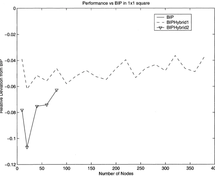
3-4 BIP example - Node 2 is added to T to and the BIP computation is complete. 35 3-5 Performance of B I P H ybrid1 and B I P H ybrid2 as compared to BIP.

3-6 Simulation Results at Infinite Range . . . . 3-7 Simulation Results at Limited range, 100 node networks 3-8 Simulation Results at Limited range, 200 node networks 3-9 Simulation Results of Multiple Source BIP . . . . 3-10 Simulation Results of Multiple Source Distributed Algorithm.

39 59 61 62 67 68

Chapter

1

Introduction

Over the past decade, research interest in the area of ad hoc networks has increased dra-matically. An ad hoc network can be described as a network that is built in the absence of preexisting infrastructure. Common examples include networks for emergency response, sensor networks and various military applications. In emergency communication networks, the following scenario is a good example: communication infrastructure has been destroyed by a natural disaster, so each rescuer is given a radio that can broadcast messages wirelessly (at some limited range), and we would like to route messages between radios that cannot directly transmit to one another. Because the infrastructure for this communication network was not built before the radios are used, this is considered an ad hoc network. Ad hoc net-works are most useful in environments where the cost of constructing a fixed communication network is too high, and too time consuming compared to deploying an ad hoc network in its place. Consequently, research in this field focuses on constructing networks that can function with minimal resources (to lower per-node cost), without sacrificing usability. Examples of

ad hoc networking issues include energy usage, wireless interference avoidance, and routing robust to mobility.

In this thesis, we are interested in the construction of energy-efficient one-to-all trees in ad hoc networks, as posed in [10]. Starting with a given source node s, the problem is to find a broadcast tree that allows s to send a message to all other nodes, using the minimum amount of energy. Although it is tempting to do so, we do not simultaneously deal with other issues such as channel contention and mobility - we believe that a well-formed solution to this problem can serve as an intuitive start to algorithms that also include other issues.

We focus on a specific type of ad hoc network where all nodes are stationary (usually referred to as a "static" ad hoc network), and equipped with an omnidirectional transmitter. We assume that the transmission range of the transmitter can be adjusted from 0 up to a maximum range

Rmax.

Although previous energy-efficient routing research has focused on environments where the transmitter can either be turned off, or transmitting at its maximum range ([11]), we adopt the model of more recent ad hoc networking research where transmit-ters are permitted to choose any range in between 0 and

Rmax

([13]-[17]). The transmitter is referred to as omnidirectional because it does not focus the message transmission in a particular direction. Therefore, when the omnidirectional transmitter sends a message at range r, all nodes within distance r can receive the message, regardless of their position. Naturally, when the node transmits a message at a higher range, it consumes more power. In analyzing the range-power tradeoff, we adopt a common communications model, where the power required to transmit the message is proportional to rCt (ex

2:

2 in all networks, and most typically is greater than 2).

2 4

Figure 1-1. The Multicast Advantage

Note that because each node can only transmit up to distance Rmax , it is possible that

the source s cannot reach all nodes in the network directly. Therefore, some nodes will have the responsibility to forward messages on the behalf of s. We can then rephrase the one-to-all problem as one of assigning each node, ni, a range ri at which to forward received messages. The total cost of the broadcast tree can then be expressed as

2:

rf.

This is a very atypical cost function for a graph connectivity problem, in that cost is

node weighted instead of edge weighted. Consider the example shown in Figure 1-1. In

this situation, we denote the cost incurred when node s transmits at a distance just large enough to reach b as Power(s, b), and define Power(s, a) analogously. If s attempts to send a message to node b, this message will not be received by node a because a's distance to s is larger than b's distance to s (das

>

dbs ). However, s could optionally transmit at Power(s, a), in which case the message would be received by both a and b (because d bs

<

das).

By transmitting to a, s can get a transmission to b for "free" because of each transmission's

omnidirectionality. In [10], this was referred to as the "multicast advantage." In general, the power required for a node s to transmit a message to a set of nodes N is max Power(s, n).

nEN

A transmission at this power will be received by all nodes in N.

prob-lem from other network connectivity probprob-lems. In the first part of this thesis, we characterize the complexity of this problem, and show it is NP-complete. Consequently, it is inefficient to find the optimal solution to this problem, as it may take exponential time. Hence, it is important to investigate the possibility of an approximation algorithm - a polynomial time algorithm that does not necessarily find the optimal solution, but constructs solutions that are not much more costly than optimal. We first look at a previously published global approximation scheme ([10)), and explore improvements to it. We then investigate a dis-tributed approximation algorithm, and show its performance is comparable to a centralized approximation ([10)) in the average case. We conclude by introducing the multiple source broadcasting problem, and explore the extent to which multiple sources can be used to save energy.

1.1 Problem Formulation

The ad hoc wireless broadcasting problem can be stated as follows: We are given a set of nodes N and a function ¢J : N -+ Z x Z, which gives us a set of coordinates for each node on the two dimensional plane. Each of these nodes represents a static (non-mobile) wireless-enabled device that is capable of both transmitting and receiving messages from its neighbors. Additionally, we are given a range

R

f Z+, which represents the maximum distance

any node can transmit a message, and a constant a

>

O. We construct the undirected graph G

=

(V, E) where V

=

Nand (i, j) f E ¢::::} dij ~ R. Assuming this graph is connected,

the wireless broadcasting problem can be stated as follows:

that connects

s

to every node in N -

{s}

via a directed path such that dij

:S

R V(i,j) tT. Given that f(x)

=

max{d~j : (x,j) tT}, we define the cost of T

as

2:

f(n).

nfN

Hereafter, we refer to the decision version of this problem, where we are asked to deter-mine whether there exists such a tree with cost less than l t Z+, as BCAST.

1.2 Background

1.2.1

Complexity

In [18], it was shown that the graph version of the BCAST problem is NP-complete. In the graph version of BCAST, we are given a directed graph with an arbitrary, nonnegative cost on each edge. Given a source s, the graph version of the BCAST problem is to construct a subset of edges E' with minimum cost (where the cost is

2:

f(n), and f(n) is the maximum

nfN

cost over all E' edges exiting node n) such that the subgraph induced by E' contains a path

s to every node. We refer to the graph version of BCAST as GENBCAST. The proof of GENBCAST's NP-completeness can be done via a simple reduction from the set cover problem ([18]).

Although the BCAST problem can be modeled as a GENBCAST problem, the NP-completeness of GEN BCAST does not necessarily imply that BCAST is NP-complete. For this to be true, we would have to prove that the G EN BC AST problem remains NP-complete for graphs that have a geometrically restricted cost function. This cost function must reflect positions of each node in the 2D plane, where the the cost of an edge

(i, j)

corresponds

to the power used in transmitting from i's position to j's position in the plane. To prove the problem remains NP-complete for graphs that are thus geometrically constricted is not trivial - as an exercise, consider the difficulty of extending GENBCAST's reduction from set cover to work for this class of cost function.

In considering the NP-completeness of BCAST, some insight can be drawn from other connectivity problems with similar cost functions. In [5], it was shown that the problem of constructing strongly connected subgraphs of minimum cost (with the same cost function as in GENBCAST) is NP-complete. That is, the problem of constructing a subset E' of directed edges, with minimum cost, such that there is a directed path from each node to every other node via edges in E ' , was proven NP-complete. Notably, the proof in [5] did not show that this problem, with geometrically restricted cost functions, was NP-complete. Rather, they proved only that the strongly connected version of GENBCAST was NP-complete.

Without further consideration, it is unclear whether or not the BC AST problem is NP-complete. On the one hand, one may argue that the geometric constraint makes the problem more tractable than the NP-complete G E N BC AST -this additional constraint can be used to eliminate many potential solutions. Quite possibly, this additional constraint might result in the existence of at most a polynomial number of feasible solutions (which would imply that BC AST can be solved in polynomial time). On the other hand, one might argue that this additional constraint has no effect on the problem's difficulty, or makes the problem more difficult than GENBCAST. Certainly, GENBCAST contains some similarities to the Steiner problem, in that "Steiner" points in a Steiner tree somewhat correspond to nodes of large transmission "radius"; both serve as points where the tree branches out to several

nodes at once. Notably, Steiner problems, when restricted to graphs in 2D, are still NP-complete ([7]). It is quite possible that GENBCAST behaves similarly when geometrically restricted.

Some understanding of how this geometric constraint affects the complexity of this class of connectivity problems was addressed in [6]; it was shown that the strongly connected version of this problem, when restricted to cost functions that reflect node positions in the plane, still remains NP-complete. Naturally, the reduction in [6] is much more complicated than the one presented in [5]. Unlike the reduction in [5], the reduction in [6] has to map each instance of an NP-complete problem to a set of node positions in the plane, which adds considerable difficulty to the proof.

In addition to constructing this mapping to node positions in the plane, the proof in [6] underwent a lengthy case-by-case analysis to demonstrate that the number of nodes being generated by their reduction is polynomially related to the size of the input (if this were not the case, the reduction would not be polynomial). Although this is an easier method of proof given the considerable complexity of any placement algorithm, the reading of the case analysis in [6] made it more difficult to ascertain exactly how the reduction was being performed. This gave us an appreciation both for the complexity of the role of the geometric constraint in BCAST, and the need for simplicity in any geometric reduction.

1.2.2

Algorithms

Most previous research on energy efficient messaging in ad hoc networks has not focused directly on problems similar to BCAST. The differences seem to lie in the model of the

energy-limited wireless environment.

For example, Das and Bhargavan adopted a model in which all nodes share a common maximum range, and a node can either not be transmitting at this maximum range, or not be transmitting at all (no range control). In [11], they look at the problem of finding a minimum sized subset of nodes that is a connected dominating set - this subset obeys that property that every node in the graph is either in this subset or in the range of a node in this subset, and that the graph induced by this subset is connected (this can be used as a "backbone" for unicast routing). Other research also adopted this model, but extended it to allow nodes to roam between several power modes, indicating their level of participation in network routing (see [12] for an example).

Later papers have extended this model to one where each node is able to transmit at any range between

a

and the maximum range. As opposed to the above model, this environment allows minimization of energy consumption at a finer granularity. Additionally, a model assuming range control allows the network designer to make the decision of providing a maximum range high enough to ensure connectivity without having to worry simultaneously about the effects on energy efficiency (granularity effects). This model is also more reflective of current low-energy transmitter technology ([13]), and many other papers have shown this model is useful for purposes other than energy savings, such as collision avoidance ([14], [16]) and quality of service ([15], [17]). For these reasons, this is the model that we have adopted in our analysis.

Work by Wieselthier, et. al. looked directly at the above broadcast problem ([10]), and proposed a centralized algorithm to construct energy efficient broadcast trees. They showed

that their algorithm, the Broadcast Incremental Protocol (BIP), performed well in practice compared to minimum spanning trees and shortest path trees. The BIP algorithm assumes the same model for power-range tradeoff that we assume in this thesis (power proportional to

rO),

so it is particularly relevant. Additionally, to our knowledge, BIP is the best known algorithm for this problem in the present literature ([18]). Consequently, we will use the performance of BIP as a measuring stick in judging our algorithms. As we will discuss below, BIP assumes that each node does not have a range limitation

(Rmax

=

(0). This is an important distinction from our problem, in which we assume that all nodes have some predefined range limit.

A year after BIP was introduced, [18] proved that the BIP algorithm has a constant approximation ratio of 12. That is, the power consumed by a broadcast tree generated by BIP is at most 12 times the power consumed by the minimum power tree. Although the value of the constant is not as important, the fact that this was a constant (i.e. not a function of the number of nodes) was significant. This differentiates the BCAST problem from other problems in wired networks that have similar characteristics, like the Directed Steiner Problem (in [8], it was proven that no polynomial time algorithm for this problem can achieve an approximation ratio better than O(lgn)). Furthermore, this gives hope that, although solving BC AST optimally is intractable, it can be approximated to within a small factor.

1.2.3 The need for a distributed algorithm

Although BIP has already been shown to construct energy efficient trees in practice ([18]), it's centralized nature requires one node to collect the position information of every node in the graph, compute the BIP tree, and distribute the solution to all other nodes in the network. This can result in considerable time, message complexity, and power consumption. Additionally, this requires that the node performing the computation also has considerable resources (energy, processor, and memory). In the low cost, resource limited environment that is typical in ad hoc networks, this may not always be feasible.

These reasons motivate a need for a localized, distributed algorithm that can compute broadcast trees without sacrificing performance. A localized algorithm is one in which nodes' decisions are based on network conditions within some limited distance. In this type of implementation, many nodes are simultaneously computing local parts of the tree, and use messages to coordinate activities with neighboring nodes. This results in considerably less computation time, message complexity, and power consumption as compared to a centralized algorithm. Such an algorithm would also use the collective resources of the network, avoiding the need to invest in costly high-resource nodes. For example, [19] presented a localized, distributed algorithm for the energy efficient unicast routing problem in networks with the same power-range tradeoff.

As part of our work, we have developed a localized, distributed algorithm that computes broadcast trees. In the first portion of the proposed distributed algorithm, nodes calcu-late a clustering on the graph. Clustering has been used as a strategy in many other ad hoc networking problems, including unicast routing, collision avoidance, and power control.

Clustering algorithms form groups of nodes, where each group contains one elected "cluster-head" node, responsible for coordinating activities on the behalf of the rest of the group. For example, clusterhead routing has been proposed to solve the unicast routing problem ([21], [11]) - packets are routed along a clusterhead "backbone" until reaching the clusterhead of the destination node's cluster. Once there, the clusterhead sends the message directly to the destination node.

In our distributed algorithm, we attempt to generate a clustering that uses minimum energy while still assigning each node to cluster. Once this clustering has been computed, clusterheads are connected together to form a broadcast tree via an extension of a well known distributed algorithm ([9]) for computing directed MSTs.

Chapter 2

Complexity

We attempt to prove the following theorem.

Theorem 1. BCAST is NP-complete.

2.1

Relevant Background Work

Before presenting the theorems and algorithms (from other papers) that we used to prove

BC AST's NP-completeness, we go over some preliminary definitions for the purposes of clarity.

Node Cover: Given an undirected graph G

=

(V, E), a node cover is a set of nodes

S ~ V such that for every edge (i, j) E E, i E S or j E S.

Connected Node Cover: A connected node cover of a graph G = (V, E) is a node cover S such that the graph induced by S on G is connected.

Connected Dominating Set: A dominating set of a graph G = (V, E) is a subset S ~ V such that every node in V is either in S or is a neighbor of a member of S. A connected

dominating set is a set S such that the subgraph induced by S is connected, and S

is a dominating set.

B

~

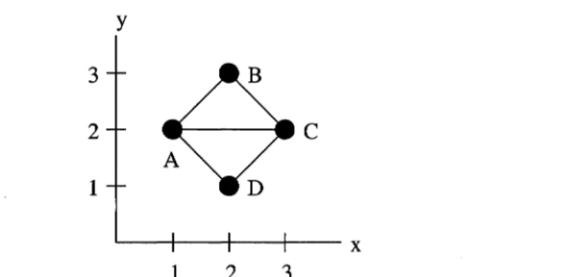
_D

Figure 2-1. The set {B, D} is a node cover of this graph G. {A, D} is a connected node cover of G. G also has a connected dominating set {C}.

Planar Graph: A planar graph G

=

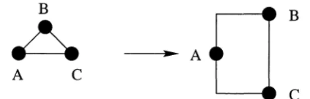
(V, E) is a graph that can be drawn in the plane without any edges overlapping. In other words, there exists a function 7rl : V -t JR x JR such that if we draw a point at 7rl (v) for all v E V, and then draw a straight line segment from 7rl (i) to 7rl (j) in the plane for all (i, j) E E, no line segments will cross. The function 7rl is referred to as a planar embedding of the planar graph G.

y 3 2

---4·c

1 '---I----I----I----x 1 2 3

Figure 2-2. G is also a planar graph. This demonstrates a planar embedding for the graph G.

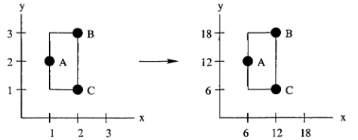
Planar Orthogonal Grid Drawing: Given a planar graph G = (V, E), a planar orthog-onal grid drawing (POGD) of G is a drawing on a grid such that each vertex is

to a sequence of horizontal and vertical grid segments, such that no two edges ever cross. y 18 B 12 6 D x 6 12 18

Figure 2-3. A POGD for the graph G.

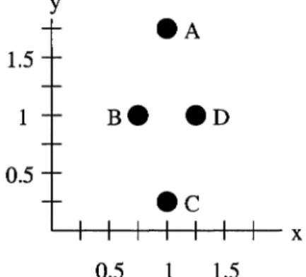
Unit Disk Graph: A graph G = (V, E) is considered a unit disk graph if there exists a mapping 1f3 : V -+ Q x Q to points on the two dimensional grid such that

(i, j)

E E 1f3 (i) and 1f3 (j) are less than distance 1 apart.

y 1.5 0.5

ec

L-.+-+-+--I-+--I--f-- X 0.5 1 1.5

Figure 2-4. An example showing G is also a unit disk graph. This is a demonstration of 11"3.

Having defined the terms above, we are now in a position to present the results of other papers used in our proof:

Theorem 2. - NP completeness of Planar Connected Node Cover Given a planar graph G

=

(V, E) of maximum degree less than or equal to

4,

determining the existence of a connected node cover V* ~ V of G such that

I

V*

I

:S k, for some given k E Z+, zs

B

A

-~ .. - A

B

A C

C

Figure 2-5. Constructing the POGD in Step 1 of the reduction.

Theorem 3. - Orthogonal Grid Drawings of Planar Graphs Given a planar graph

G = (V, E) of maximum degree less than or equal to

4,

an orthogonal grid drawing of this graph can be drawn in polynomial time, such that the size of the grid is polynomial in

IVI.

Proved in [3].

Theorem 4. - Connected Domination in Unit Disk Graphs Finding a minimum sized connected dominating set of a unit disk graph is NP-complete. We refer to the decision ver-sian of the connected dominating set problem (i. e. "does there exist a connected dominating set of size no more that k,?") as CDSUDG. We reproduce the reduction used in the proof of this theorem (from

!4])

below.

Proof of Theorem 4: We now describe the reduction used in Clark, et al. in [4] to prove Theorem 4.

Given an instance of PLAN AR, with graph G

=

(V, E), maximum node cover size k € Z+, we convert it to an instance of the C DSU DG problem as follows.

1. We first construct the POGD of G using the algorithm mentioned in Theorem 3 (this is done on an example graph in Figure 2-5).

2. We then multiply the size of the grid by 6 so that each line segment of length one is mapped to a segment of length 6. This illustrated in Figure 2-6.

y y 3 18 2 _{- - - 12} 6 '---+--f---+--x '---+--f---+-- x 1 2 3 6 12 18

Figure 2-6. Multiplying the grid size in Step 2 of the reduction.

Y node region of A y 20 \ • • • • • • • pL2(B)

::~{

6 C

-:: !!'!:

• •

I

•

•

i 2(A) • • x P - • • • • • • • pi_2(C) 12 18 5 10 15 20

Figure 2-7. Step 3 of the reduction. P is the set of nodes in the graph on the right. The end nodes in A's node region are at (6,11) and (6,13).

3. Place a node at every grid point in the POGD, and denote this set of nodes as P (For example, if the line segment from (0,0) to (0,2) is in the orthogonal grid drawing, P contains nodes at positions (0,0), (0,1), and (0,2)). Note that each vertex v E V in the instance of

PLAN AR maps to a node in PEP such that 7r2 (v)

=

P (where 7r2 is the function in the definition of a POG D). For each PEP such that 7r2 (v)

=

P for some v E V, we refer to p and all nodes in P that are within 1 grid length of p as the node region of v. Those nodes that are in the node region by virtue of being within 1 grid length of p are called the end nodes of that node region. The other node (the one that is mapped to from V via 7r2) is referred to as the center node of this node region. See Figure 2-7.

4. We then construct the set PI as follows. Construct the subset pI C P, which contains all nodes in P that are not in node regions. Also, for future reference, we denote the set

20 20 B o B

: .... ++

0 • • • • •

++

O. 000

•

•

O. O. 15

•

•

15 O. O.

•

•

O. O.

Ai

•

Ai

O.

•

O.

•

O. 10

•

•

10 .0 O.

•

•

.0 O.

•

•

.0 .0 : •••• +1= O. +1=

•••••

c 00000 c 5 W ~ 5 W ~ w

Figure 2-8. Step 4 of the reduction. Black nodes are nodes in pI, and Pl nodes are white. Nodes denoted with a "+" are in node regions.

that 1) each Pl node is placed at a grid point, 2) for each node in pI there is exactly one

node in

P"

located one grid length away, 3) for each node in

P"

there is exactly one node in pI located one grid length away, and 4) no node in

P"

is within one grid length of any node in P - P'. This operation effectively creates a "layer" of nodes around the original POGD's

edges, which is why we use the subscript l.

To complete the reduction, we construct a unit disk graph so that every node in P U Pl

corresponds to a node in the unit disk graph, and edge (i,

j)

exists in the unit disk graph iff i and j's corresponding nodes are within distance 1 of each other. This completes the reduction used in Theorem 4.

Denote

IVI

as the total number of nodes in the original PLANAR instance, and

lEI

as the total number of edges. In the last step of the reduction in [4], the following lemma was proved:

Lemma 1. There is a vertex cover of size no more than k in the original PLAN AR instance iff there is a connected dominating set in the corresponding unit disk graph of size no more than

IVI-IEI-1 +

k

+

IP"I·

2.2

Proof of NP-completeness

We construct a reduction from PLANAR to BCAST inspired by the reduction used in Theorem 4 ([4]), showing that we can convert any instance of PLANAR into an appropriate instance of BC AST in polynomial time. We confirm the correctness of our transformation by showing that every positive instance of PLANAR maps to a positive instance of BCAST,

and that every negative instance of PLANAR maps to a negative instance of BCAST. This demonstrates that BCAST is NP-hard. We go on to prove that it is NP-complete (thereby proving Theorem 1) by showing BCASTENP.

The reduction In proving the NP-hardness of BCAST, we can extend the reduction in [4] and use some of the properties derived there to prove the correctness of our reduction.

To extend the reduction in [4], we construct the BCAST instance from PLANAR in-stance as follows. First, we perform the reduction in [4] to an inin-stance of CDSUDG. We then modify this reduction as follows:

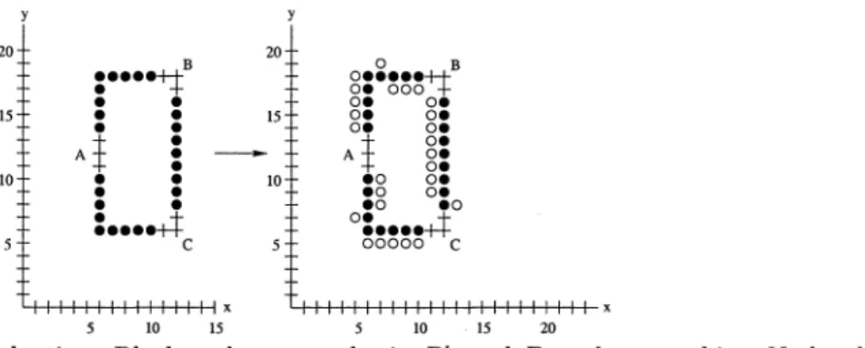
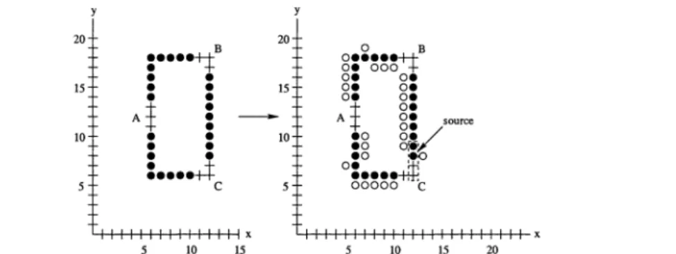
Choose an arbitrary magnified POGD edge segment such that one end of the segment corre-sponds to a center node position (note that the POGD is magnified six times, so it must be 6 grid units long, and contain 6 nodes). Denote the first four nodes in P along this POGD seg-ment (starting from the center node) as nI, n2, n3 and n4. Hence, nI corresponds to a center node, and n2 to an end node. Adjust the PI nodes corresponding to n3 and n4 so that they are not within one grid length of each other. Note that this adjustment to the CDSUDG

instance can be done for any

Il,

while still satisfying the other conditions required of nodes in Pl. Therefore, the CDSUDG instance is still valid after this adjustment has been made,

20 15 10

:····+l

•

•

•

•

•

•

Ai

:

•

•

•

•

•

•

: •••• 4

_c '-I+-H+-H+-H+-H-H x 20 15 10 o B O •••• e++ O. 000·+ O. O. O. O. O. O.

i

O. A O. source 0 • . / . 0 O. .0 oie' 0:0 :ep

~~~~~-ti:P.C

w ti W ti 20

Figure 2-9. Step 4 of the reduction, with a box around the nodes nl through n4. Black nodes are nodes in

pi, and Pt nodes are white. Nodes denoted with a

"+"

are in node regions.

and all proofs concerning the CDSUDG instance ([4]) still hold for this modified reduction.

We then extend the instance of CDSUDG to a corresponding BCAST instance as

fol-lows:

1. The nodes of the BCAST instance are the same as those in the modified CDSUDG

instance (note that this is valid because each node in the generated CDSUDG instance is

located at integer coordinates).

2. Set the source node of the BCAST instance, s, to be n3 from above. This is demon-strated in Figure 2-9, where the source is chosen to be at (12, 8).

3. The range of each BCAST node is set to 1 grid length.

Note that even with the addition of these steps, the total time for the reduction is still polynomial.

Proving NP-hardness from this reduction Assume that we have taken a PLAN AR

instance and converted it to an instance of CDSUDG, and then extended the CDSUDG

instance as noted above to construct an instance of BC AST. Then the following lemma

holds:

iff there exists a connected node cover of size no more than k in the original instance of PLANAR.

Proof: Note the following observations about the BCAST instance constructed:

Observation 1: All neighbors of a node in the instance of CDSUDG are at distance

exactly 1. Because the range of each node in the BCAST instance is 1, this implies that in any BC AST tree, a given node is either using 1 unit of power or 0 units of power. Therefore, we can consider a node in the BC AST instance as either being "on" or "off".

Observation 2: The source node must be included in any connected dominating set in the generated instance of CDSUDG (because it is the sole node within one grid length of its corresponding Pl node).

Observation 3: Any connected dominating set CDS for the instance of C DSU DG can be mapped to a valid tree in the matching BC AST problem. To do so, turn on only those nodes in the BCAST instance that are in CDS. This is a valid BCAST tree because it includes the source s as turned "on" (by Observation 2), and for a given node, n, in the

BCAST instance there is a path from s to n via "on" nodes (by virtue of CDS being a connected dominating set). Additionally, the number of elements in CDS is equal to the power used in the BC AST instance (by Observation 1). Therefore, every solution to the generated CDSUDG instance maps to a corresponding BCAST solution. We can also prove the converse statement. To prove this, note that the "on" nodes in a BC AST solution must constitute a dominating set (otherwise, there is a node which cannot be reached by the source in the BCAST solution, implying it is invalid). Additionally, in any valid BCAST

is also connected. Therefore, we can map a BCAST solution to a CDS in the matching

CDSUDC problem by selecting the set of "on" nodes. Note that the power used in the

BCAST solution is exactly equal to the cardinality of the CDS that it maps to.

Observation 3 implies that there exists a connected dominating set of size no more than

J in the CDSU DC instance iff the corresponding instance of BCAST contains a broadcast tree of power no more than J. This statement, taken together with Lemma 1, implies Lemma 2 . •

Lemmas 1 and 2 imply that we can map every instance of PLANAR to an instance of

BCAST in polynomial time, proving that BCAST is indeed NP-hard. Also, note that the coordinates of each BC AST node generated this way have size that is at most a polynomial function in the number of nodes (because in [3], the size of the POGD is polynomial in the number of nodes). This fact further implies that BCAST is strongly NP-hard (see [2] for a definition of strong NP-hardness).

We show BCAST is strongly NP-complete, by demonstrating that BCASTENP. We show this by demonstrating that there is a polynomial time verifier for BCAST. Given a

BCAST tree rooted at source s, with range R, and total power allotment l, we can compute whether this is a valid tree (no node transmitting beyond

R

distance, and all nodes reached via a directed path from

s),

and also compute its total cost, in polynomial time. This is all that we must do to verify that a given BC AST tree is a valid solution for a specific instance of BCAST. This completes the proof of Theorem 1. •

Chapter 3

Constructing Broadcast Trees

3.1

The Broadcast Incremental Protocol (BIP)

In light of the NP-completeness of BeAST, the fact that BIP achieves a constant approxi-mation ratio is remarkable. It is even more impressive given the algorithm's simplicity. BIP ([10]) performs much like Prim's algorithm for constructing MST's ([20]). BIP grows a tree from the source, and augments the tree with the node that can be added with the least

additional cost. It continues to add one node at a time until all nodes have been added to the tree. Once the tree is complete, a very simple "sweep" procedure traverses the tree and lowers power in cases of overlap, while still ensuring there is a path from the source to every node.

Throughout its execution, BIP maintains a set of nodes T that denote the tree made so far. Additionally, it maintains a power level Pi for each node in T (initially, T

=

{s}

and

node n E N - T. Specifically, BIP increases the power of the node

t

that requires the least

additional power to reach a node in N - T (the additional power for t to reach node n is Power(t, n) - Pt). Once the node pair (n, t) that requires the least additional power has been identified, n is added to T with Pn

=

0, and Pt is increased to Power(t, n). This process continues until T

=

N.

Consider the following example, where we assume the power to transmit at distance d is

exactly d2 : 4

02

sO 2

10

30

2 4

Figure 3-1. BIP example - the starting configuration.

Initially, T =

{s}

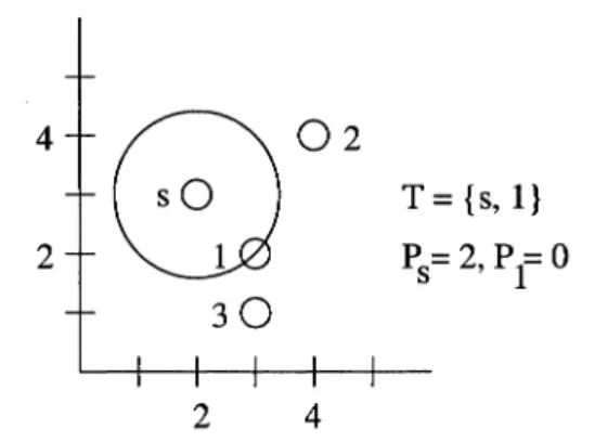
and Ps = 0, so the additional costs to add nodes 1, 2, and 3 from s are 2, 5, and 5 respectively. For this reason, node 1 is added to T and Ps is set to 2 (as shown in Figure 3-2) . 4

8°2

sO T = {s, I} 2 1 P_s=2,PtO

30

2 4

Figure 3-2. BIP example - Node 1 is added to T.

and 5 - Ps = 3 respectively. Similarly, the additional cost to add nodes 2 and 3 from node 1 are 5 and 1 respectively. The minimum of these four values is the additional cost to add 3 via a power increase at node 1. Therefore, this power increase is chosen (see Figure 3-3).

4

T

=

{s, 1,3}

2 _{Ps= 2,}

_Pt

_{1, P3=}

°

2 4

Figure 3-3. BIP example - Node 3 is added to T.

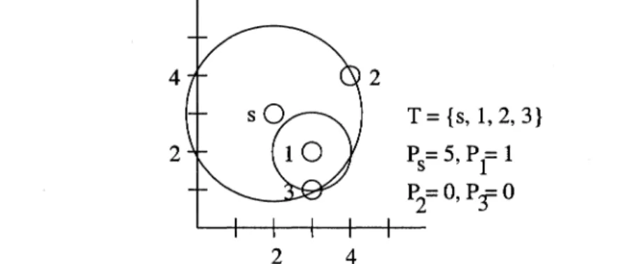
At this point, the additional cost to add node 2 from nodes s, 1, and 3 are 3, are 5-ps = 3, 5 - PI

=

4 and 10 - P3

=

10 respectively. Therefore node 2 is added by increasing the power of node s to 5, and the final tree is as represented in Figure 3-4.

4 2 2 2 4 T

=

{s, 1, 2, 3} Ps= 5,

Pt

1 P2=O, P:f 0

Figure 3-4. BIP example - Node 2 is added to T to and the BIP computation is complete.

Note that the tree we have made is a valid BeAST tree - there is a path from s to all

nodes in the graph. Additionally, note that we never specified the range Rmax - BIP assumes

that nodes do not have a range limitation. That is, each node can always transmit to any other node as long as it uses enough power. As we look at improving BIP, we will focus on algorithms where we assume the BIP environment (no range limitation). However, when

de-veloping a distributed algorithm for the purposes of feasibility in real-world implementation, we will include the range restriction, as this is more representative of real-world transmitter limitations.

In our example, notice that the cost of the BIP tree can be improved, by observing that the node 1 need not be transmitting. This is because node s is already able to reach node 3 and node 1. Therefore we can turn off node 1 and still have a path to node 3 from s. This "overlap" situation commonly occurs in trees constructed via BIP. Consequently, the authors of BIP introduced a "sweep" algorithm ([10)). After BIP has constructed a tree, the sweep algorithm looks for situations similar to the one in our example, and reduces the power of certain nodes in the tree without making the tree invalid. In particular, sweep looks for the following general condition: Let hi be the minimum number of hops needed to receive a message from s at node i in the given tree, and refer to the condition Pi ~ Power(i,j)

as i covering j. Then, if there are nodes i, j and k such that 1) hi

>

hj, 2) i covers k and 3) k is the farthest node from j such that j covers k, then reduce the power of j so it no longer covers k. In other words, if there is an upstream node i and a downstream node j

both covering the same node, then sweep checks to see if j's power can be reduced (note that the upstream/downstream requirements ensure that s will still have a path to this "doubly covered" node after the power decrease). This algorithm significantly improves the average cost of trees generated by BIP.

3.1.1

Improving BIP: Hybrid Algorithms

As said previously, BIP is an astonishingly simple greedy algorithm. Especially given the NP-completeness of the BeAST problem, it is surprising that BIP does not have to exhaustively tryout a series of choices at each step to determine which will be most beneficial at later iterations. Even without such behavior it still performs well. Consider what would happen if we performed a limited exhaustive search in the earlier stages of the algorithm, and then allowed BIP to continue with greedy choices after some point. This is the sort of algorithm we had in mind when constructing a BIP hybrid.

In this algorithm, which we call BIPHybrid1, an initial power assignment and partial

tree T is constructed, which is then "completed" by running BIP. To construct a tree, we assign the source a power level. Once this power level has been chosen, Ps is set to this power, and T is set to include the source and all nodes reached by the source at this power (all non-source nodes that are in T are set to have zero power initially). Then, BIP is run with this starting

T

and power assignment. Once the BIP algorithm terminates, we have constructed a tree. In BIPHybrid1, this procedure is repeated for all N -1 possible power

levels that the source may be set to. Then the minimum power tree (among the N - 1 trees thus generated) is returned.

We also looked at an extension of BIPHybrid1 , which we refer to as BIPHybrid2 • In this algorithm, a similar procedure is performed, except the initial tree

T

is made by setting the power of the source, and then setting the power of a node that is reachable from the source. Then BIP is run to "complete" this initial tree. This procedure is then repeated to for all possible initial trees (in which two nodes are on). The lowest energy tree is then

returned. Note that this means that the cost of the BI P H ybrid2 tree is never more than the cost of the B I P H ybrid1 tree (for the same problem instance).

By looking at these two algorithms, we can get a sense of how far BIP is from the optimal solution. If we notice that the cost savings (compared to BIP) grows very quickly going from

BI P H ybrid1 to BI P H ybrid2 , we have reason to believe that BIP constructs trees with cost

much higher than the optimal solution. Likewise, if the cost savings does not grow quickly, we have a rough "sense" that BIP performs close to optimal on average. We simulated the performance of BIP, BI P Hybrid1 and BI P Hybrid2 for various size networks confined to a lxl grid. After each algorithm was run, the BIP "sweep" algorithm was run on the tree.

As we can see from Figure 3-5, BI P H ybrid1 is a 5% improvement on BIP, and this does

not change as a function of instance size. This indicates that the power of the source's trans-mission can have a significant impact on power efficiency. Note that BI P H ybrid2 doesn't add

much additional improvement - it averages to about another 2% savings over BIPHybridl .

Unfortunately, due to the computational resources required, we couldn't measure the per-formance of B I P H ybrid2 for larger instances. However, the lack of additional savings going

from B I P H ybrid1 to B I P H ybrid2 seems to indicate that BIP does not significantly deviate

from optimal in the average case.

3.2

Computing Broadcast Trees Distributively

In this section, we describe a localized, distributed algorithm that computes broadcast trees. In the first portion of the proposed distributed algorithm, nodes calculate a clustering on the graph. Then, the clusters are joined together using a well known distributed algorithm

Performance vs SIP in 1 x1 square O~---.---.---.---.---r---'---.---~ -0.02 a.. -0.04 iii E

,g

c o

~

-0.06 Q) o Q) > ~ Q) a:: -0.08 -0.1 II ... / / ... / /

-/ / / / '" / \ \ \ / '" - S I P - - SIPHybrid1 ~ SIPHybrid2 I '\ I '\ I I _0.12L---L---L---L---~---~---~---~----~

o

50 100 150 200 Number of Nodes 250 300

Figure 3-5. Performance of BIPHybrid1 and BIPHybrid2 as compared to BIP.

for computing directed minimum spanning trees.

350

At the beginning of the algorithm we assume each node has the following information:

1. Each node i knows the distance to every node in i's neighborhood. A node's neigh-borhood is defined as the set of nodes that are within distance R (the maximum distance that a node can transmit a message). Nodes that are in i's neighborhood are referred to as neighbors of i.

2. Each node i also knows the distance of each neighbor to every node in the neighbor's 400

neighborhood. We refer to the set of i's neighbors, and i's neighbors' neighbors as i's

two-hop neighborhood.

As an example, this information could be gathered by determining pairwise node delay via timestamps. Notice that each node only requires localized information about some small portion of the network (the two hop neighborhood). This is a key difference from previous algorithms like BIP, which require each node to have global network information. Also, note that this is only meaningful in networks with limited range - if each node had unlimited range, having two-hop neighborhood information would be equivalent to having global information. In networks with limited range however, the two-hop neighborhood may constitute a small fraction of the graph. Of course, this also holds for networks in which the range of nodes is limited for reasons other than inherent transmitter limitations (like avoiding interference).

In our initial development of a distributed algorithm, we assume that the network is synchronized via a global clock, no messages are lost, and that there is no interference. We then extend the algorithm to work without the benefit of a global clock in networks where interference and packet loss is possible.

3.2.1

The formation of

cl

listers

In the first phase of the algorithm, a clustering is constructed on the nodes using the afore-mentioned distance information. Once this phase is complete, each node will be assigned to at least one cluster, and each cluster will have one "cluster head" node. We define the cost of a particular cluster as the power required for the clusterhead node to transmit to all other nodes in the cluster (in one transmission). In addition, we consider the cost of a particular

clustering to be the sum of the costs of its clusters. Given this cost function, we attempt to develop a minimum cost clustering.

Before describing our distributed clustering algorithm, we first describe a centralized clustering scheme. A simple centralized algorithm can be described as follows: Throughout the execution of the algorithm, each node i's range is referred to as ri, and each node is either unmarked or marked, reflecting its membership in a cluster. The algorithm begins with ri

=

0 for all i, and all nodes unmarked, and proceeds as follows:

1. For each node i, compute the function ai(r). If i was to increase its range to r, this function represents the average cost induced per unmarked node within distance r of i. More precisely,

a.(r) = P(r)-P(r;) t Ui(ri,r)

where P(x)

=

power to transmit at range x

Ui(XI, X2) = number of unmarked nodes in between distances Xl and X2 of i

ri

=

node i's present transmission range

2. For each node i, compute the range at which ai(r) is minimized. This is the most cost efficient range increase (in a greedy sense) for node i. Denote this range as rmini, and the value of a at this range as amini.

3. Find the node j that has the smallest value of amin - this is the node that (globally) has the most cost efficient range increase. Increase r j to rminj, and mark nodes j and

all nodes within distance rminj of j.

4. Repeat steps 1-3 until all nodes are marked.

Once the above algorithm terminates, the final ri values specify a clustering (because

nodes are only marked if they belong to a cluster). Each node with nonzero ri is considered

a clusterhead, and all nodes within distance ri of i are considered members of i's cluster

(note that, in our algorithm, a particular node may be a member of more than one cluster). Because we greedily choose the range increase that minimizes the average additional cost induced per node marked, we are hopeful that the clustering produced is cost-efficient.

Interestingly, the greedy behavior of the above algorithm can be implemented distribu-tively, with one important difference. In a distributed implementation it is very costly (in message complexity) to compute a global minimum - therefore, the distributed algorithm (described below) attempts to find local minima instead. Although this may result in less

power efficient clusterings, such inefficiencies are inherent to many localized algorithms.

3.2.2

Synchronous Distributed Clustering Algorithm

As in the global algorithm, each node i maintains a range value ri initially set to 0, and is

initially unmarked. Additionally, we ensure that each node i maintains up-to-date values of: 1) rj for all neighbors j, and 2) MARKED status of all nodes in the two-hop neighborhood. The algorithm we propose operates in stages. During each stage, local minima are computed, and the ranges of some nodes are consequently increased. Information about the range increases are then propagated. Once this has been completed, each node has updated its state information to reflect the last stage's changes, and the next stage begins.

Note that because we are assuming that all nodes are synchronized, we describe the algorithm in stages and substages where each stage and substage begin on predefined clock boundaries. In each stage, each node executes the following substages:

Substage 1. If i is unmarked, node i computes, for each neighbor j, the minimum value

of CYj(r) for r

2:

distance(i,j). That is, i finds the most cost efficient range increase

for j, looking only at those ranges that would allow i to be a member of j's cluster. Denote the value of the range and CY found through this computation as rminj-ti and

aminj-ti, respectively.

Each node i then finds the neighbor node k with minimum value of amink-ti, and sends

k a PREFERRED message containing range value rmink-ti. This message is sent at maximum power.

If i is marked already, it does not participate in this substage.

In addition each node i (marked or unmarked) executes the following steps:

Substage 2. At this substage, i has received all PREFERRED messages from its unmarked neighbors. If i receives a PREFERRED message with range value r' from all unmarked nodes within distance r' (indicating that i is a local minima), i increases ri to the value

r'o Upon increase, it transmits a RANGEJ:NCREASE message at maximum power, telling all neighbor nodes that i has increased its range to r'o If i is not already a member of a cluster, it also broadcasts a MARKED_STATUS message to its two-hop neighborhood, indicating that i has been marked (by virtue of becoming a clusterhead).

the distance from i to j is less than the new value of rj, i is a member of j's clus-ter. Consequently, if i is not already a member of another cluster, it broadcasts MARKED_STATUS message to its two-hop neighborhood, indicating that i has been newly marked. Additionally, at this substage, i may receive a MARKED_STATUS message from a neighbor that has just become a clusterhead (in the previous sub-stage). It forwards this message at maximum power (to ensure that it goes to all nodes two hops away from the clusterhead).

Substage 4. At this substage, each node i may receive a MARKED_STATUS message from a newly marked neighbor j. It retransmits this message at maximum power, to ensure that it reaches j's two hop neighborhood. At the next substage, all messages will have reached their intended receivers. Therefore, in the next substage, each node i will have up to date information on rj for all neighbors j, and the MARKED status of every node in the two hop neighborhood. After this substage, a new stage begins.

The algorithm terminates once all nodes have been marked (and hence no PREFERRED messages are being generated). Because nodes only mark themselves when they have become a member of a cluster, this also means that, upon termination, the final values of ri produce a clustering. Note the following properties of this algorithm:

A. The algorithm terminates in a linear number of stages. Consider any stage of the algorithm where not all nodes have been marked. We show that at least one new node will be marked in this stage. Let amini be the minimum value of O!i for node i. There must exist some node j for which aminj is minimum over all nodes. Because this is the global minimum, in the next stage, all unmarked nodes within distance rminj

of j will send j a PREFERRED message with range value rminj (if not, aminj would not have been the global minimum). Therefore, in the next stage, j will increase its range, and some set of previously unmarked nodes will be newly marked. This further implies that in every stage, at least one node is marked, completing the proof.

B. The algorithm uses

O(N2)

messages. In each stage, there is at most 1 PRE-FERRED message and 1 RANGEJ:NCREASE message per unmarked node, result-ing in

O(N)

messages per node per stage, and

O(N2)

messages total. Addition-ally, each node transmits a MARKED_STATUS message when it has been marked (this occurs once per node throughout the algorithm). Because each node has two-hop neighborhood information, it can compute a spanning tree upon which to for-ward this MARKED_STATUS message. Therefore, it takes at most

O(N)

messages to forward the MARKED_STATUS message to the two-hop neighborhood. Hence, we have at most

O(N2)

total MARKED_STATUS messages, and

O(N2)

total PRE-FERRED /RANG EJ:NCREASE messages.

3.2.3 Implementation Considerations

Although this synchronous algorithm works fine when there is a global clock and we assume no messages are lost or reordered, this is not at all a reasonable expectation of real-world environments. In the real world, keeping global clocks up to date requires considerable message complexity and node coordination. Additionally, messages can be lost in wireless communication, requiring retransmissions that cause arbitrary message delays.

arbitrary message delays (but not message loss) we can note the following. In the absence of a global clock, the sole difference from the synchronous case is that different nodes might simultaneously be at different stages of the algorithm (one node might be in stage 4, substage 2, while another is at stage 7, substage 1). Because nodes are "out of sync", this could lead to node decisions being made with incomplete or conflicting state information, resulting in a different tree (different from the synchronous algorithm). We can remedy this situation by using the receipt of a message as a virtual clock signal, implemented with the following rule:

Each node n is not allowed to enter a particular substage until all messages that could conceivably be destined for n (and sent off by other nodes as the result of a

previous substage) have been received.

This ensures: 1) each node doesn't make a decision until all state information from previous stages has been received, and 2) no node can be more than one stage ahead of its neighbors.

Note that in a network where all messages are guaranteed to arrive at their destination within 8 seconds, this rule would be equivalent to requiring each node to wait 8 seconds before proceeding to the next substage. In such a network, this behavior would ensure the algorithm constructs the same tree as in the synchronous case, solely because the message schedules are identical (and consequently, nodes are not out of sync). Furthermore, note that the implementation of this rule in any network (with any message delivery guarantee), would result in an identical message schedule, and consequently result in the same tree produced by the synchronous algorithm.

algorithm that obeys this rule. We can do this as follows. Assume that every node has up to date information from the previous stage (values of ri for each neighbor, and MARKED

status of each node in the two hop neighborhood). Then, each node does the following:

1. In the beginning of the stage, each unmarked node sends a PREFFERED message as in the synchronous algorithm. Marked nodes do not perform any operation. Each node is then not allowed to continue until it has received all PREFERRED messages from its unmarked neighbors.

2. Once this has occurred, if this node is going to increase its range, it sends off a RANGEJ:NCREASE message as in the synchronous algorithm. If it will not increase its range, the node sends a message to indicate this. As before, this node is not al-lowed to continue to the next step until a message is received from every neighbor node pertaining to the neighbor's range decision.

3. Once this node is allowed to continue, it sends off a MARKED_STATUS message

only if it was unmarked in the last stage. This message will indicate if this node was

marked in this stage. The node then suspends its operation until it has received a MARKEDJ3TATUS message from every unmarked neighbor.

4. Once its operation is allowed to continue, this node composes and sends a STA-TUS_SUMMARY message, which lists all nodes that have been marked in this stage (this ensures that a MARKED_STATUS update from a node travels two hops). Note that if we immediately forwarded the MARKEDJ3TATUS message without compos-ing a summary, this could potentially mean that each node sends off 0 (n) messages in

this step (increasing the overall message complexity to O(n3 )). However, if we com-pose a summary, this is reduced to 1 message sent per node, and an overall message complexity of O(n2 ).

5. This node is then not allowed to enter the next stage until a STATUS_SUMMARY message has been received from all neighbors (note that once this is done, the node has received all messages destined for it in this stage, and therefore has up to date information and is prepared for the next stage).

This algorithm ensures that no two neighbor nodes are out of sync by more than one substage, regardless of message delay. Note that the algorithm obeys the above rule, and therefore constructs the same tree as the synchronous algorithm.

Since the above algorithm tolerates messages delivered with arbitrary delay, it can further be extended to tolerate networks where messages can be lost through the use of a link-layer retransmission protocol (ARQ). Such a protocol guarantees the eventual delivery of packets, although the delivery time of the packet may vary based on the need for retransmission. However, since the above algorithm can tolerate packets that are arbitrarily delayed, we are assured that it will terminate successfully.

3.2.4 An alternate clustering algorithm

Although the above algorithm can tolerate interference and message loss, it may do so at the cost of many ARQ retransmits. This is especially of concern since most messages are being sent within each node's two hop neighborhood, increasing the likelihood for message interfer-ence and subsequent message loss. In addition to wasting energy resources via retransmits,