HAL Id: hal-01072160
https://hal.inria.fr/hal-01072160v2
Submitted on 20 Apr 2020
HAL is a multi-disciplinary open access
archive for the deposit and dissemination of
sci-entific research documents, whether they are
pub-lished or not. The documents may come from
teaching and research institutions in France or
abroad, or from public or private research centers.
L’archive ouverte pluridisciplinaire HAL, est
destinée au dépôt et à la diffusion de documents
scientifiques de niveau recherche, publiés ou non,
émanant des établissements d’enseignement et de
recherche français ou étrangers, des laboratoires
publics ou privés.
Efficient Low Cost Range-Based Localization Algorithm
for Ad-hoc Wireless Sensors Networks
Abdulhalim Dandoush, Mohamed Elgamel
To cite this version:
Abdulhalim Dandoush, Mohamed Elgamel. Efficient Low Cost Range-Based Localization Algorithm
for Ad-hoc Wireless Sensors Networks. [Research Report] Inria. 2014, pp.25. �hal-01072160v2�
Efficient Low Cost Range-Based Localization Algorithm for Ad-hoc
Wireless Sensors Networks
∗Abdulhalim Dandoush and Mohamed Elgamel
∗INRIA Sophia-Antipolis Méditerranée
2004 Route des Lucioles BP93 06902 SOPHIA ANTIPOLIS, France
[email protected] University of Louisiana at Lafayette
P.O. Box 43004 Lafayette, LA 70504 USA
Abstract
Building an efficient node localization system in wireless sensor networks is facing several chal-lenges. For example, calculating the square root consumes computational resources and utilizing flooding techniques to broadcast nodes location wastes bandwidth and energy. Reducing computa-tional complexity and communication overhead is essential in order to reduce power consumption, extend the life time of the battery operated nodes, and improve the performance of the lim-ited computational resources of these sensor nodes. In this paper, we revise the mathematical model,the analysis and the simulation experiments of the Trigonometric based Ad-hoc Localiza-tion System (TALS), a range-based localizaLocaliza-tion system presented previously. Furthermore, the study is extended, and a new technique to optimize the system is proposed. An analysis and an extensive simulation for the optimized TALS (OTALS) is presented showing its cost, accuracy, and efficiency, thus deducing the impact of its parameters on performance. Hence, the contribution of this work can be summarized as follows: 1) Proposing and employing a novel modified Manhattan distance norm in the TALS localization process. 2) Analyzing and simulating of OTALS showing its computational cost and accuracy and comparing them with other related work. 3) Studying the impacts of different parameters like anchor density, node density, noisy measurements, trans-mission range, and non-convex network areas. 4) Extending our previous joint work, TALS, to consider base anchors to be located in positions other than the origin and analyzing this work to illustrate the possibility of selecting a wrong quadrant at the first iteration and how this problem is overcome. Through mathematical analysis and intensive simulation, OTALS proved to be it-erative, distributed, and computationally simple. It presented superior performance compared to other localization techniques.
Keywords: Wireless Sensor Networks, WSNs, Range-based Localization, Distributed
Localization, Anchor-based Localization, Simulation, distance measure, Modified Manhattan, Performance Evaluation
1. Introduction and motivation
The advancement of embedded systems and wireless communication brought forth wireless sensor networks (WSN). These wireless sensor devices are deployed in plethora of applications ranging from civil solutions to military applications. Target localization and real time target tracking are widely adopted applications for wireless sensors networks. Possessing the knowledge
of the node’s location is a key parameter in these applications and in several routing algorithms [? ]. The ad-hoc nature of the sensor devices makes self-positioning an integral part of their applications.
The basic idea used in a node localization system is to measure a physical quantity, e.g. signal strength, that is proportional to distance and use the measured value to estimate the distance to a reference point. Once the distance to at least three reference points is known, the position of the tracked node can be determined.
Thus, the WSN localization process consists typically of three phases (𝑖) coordination (e.g. clock synchronization, notification of the need to localize a position) [? ? ], (𝑖𝑖) measurement of a physical quantity (and the transmission of a signal followed by signal processing), and (𝑖𝑖𝑖) position estimation [? ]. Initializing a localization process requires the coordination of some nodes. One or more nodes then emit a signal, and a property of the signal (e.g. arrival time, phase, signal strength, etc.) is observed by one or more receivers. Next, to determine the location of a node, signal measurements have to be transformed into position estimates by means of a localization algorithm. As mentioned previously, to achieve these phases correctly the existence of cooperating sensor nodes deployed into the environment at known positions a priori is essential. These nodes are called reference points or anchor nodes. The location of an anchor node can be defined through a Global Positioning System (GPS), or manually predefined, or calculated during localization system operations.
Building an efficient node localization system in wireless sensor networks is facing several chal-lenges. For example, reducing communication overhead in the two first phases of the localization process and computational complexity in the third phase is essential to reduce the power con-sumption, extend the lifetime of battery operated nodes and improve the performance of limited computational resources nodes. Typically, deployments of WSNs exist in harsh environments where nodes are subject to measurement errors due to instrumentation and communication noise. Moreover, WSN nodes are subject to destruction due to environmental effects and dead batteries. To address these challenges and be able to overcome the problems of measurements errors and communication noises of sensor nodes, the redundancy of sensor nodes and information fusion are of great use and are employed in several WSN applications. Node redundancy and information fusion techniques can enhance the quality of the estimates by avoiding outliers and substitute missing information caused by network congestion.
The following is a summary of the challenges faced in building a node localization system • Flooding: Anchor nodes flood the network with their positions, this wastes energy and
bandwidth communication [? ].
• Solving a linear system of equations: A system of linear equations is solved using the least square approximations which pose a huge computational overhead [? ].
• Finding shortest path: Computing the shortest path between anchor nodes to infer ranging estimates wastes communication bandwidth [? ].
• Square root operations: A computational intensive task that does not suit WSN devices. • High erroneous measurements: That poses a threat on the accuracy of the estimation process.
Therefore, proposing novel simple methods that can improve the localization accuracy with low cost is still a research challenge. In a preliminary joint work in [? ], TALS is proposed to address the above challenges. TALS is an anchor based localization system to address the current existing localization systems deficiencies. It utilizes ranging measurements, trigonometric functions and square distance comparisons. Moreover, a data fusion technique is applied to the different redundant estimates of each node to come out with one accurate estimate of the node location. Nodes that their location have been estimated are upgraded to become anchor nodes and aid in the localization algorithm. In this study we introduce a novel distance measurement technique to the TALS localization system, that can be seen as a modified Manhattan (MM) distance measurement technique. MM is used in calculating and comparing two distances as the
localization algorithm under consideration does not need the exact distance calculation for the comparison purpose. It does care about which estimated point is closer to the actual one in order to move to. The optimized TALS (OTALS) localization system is described and its performance is evaluated.
In this paper, we revise the mathematical model,the analysis and the simulation experiments of the Trigonometric based Ad-hoc Localization System (TALS), a range-based localization system presented previously. Furthermore, the study is extended, and a new technique to optimize the system is proposed. An analysis and an extensive simulation for the optimized TALS (OTALS) is presented showing its cost, accuracy, and efficiency, thus deducing the impact of its parameters on performance. Hence, the contribution of this work can be summarized as follows: 1) Proposing and employing a novel modified Manhattan distance norm in the TALS localization process. 2) Analysis and simulation of Optimized TALS showing its computational cost and comparing its accuracy with other related work. 3) Studying the impacts of different parameters like anchor density, node density, noisy measurements, transmission range, and non-convex network areas. 4) Extending our previous joint work, TALS, to consider base anchors to be located in positions other than the origin and analyzing this work to illustrate the possibility of selecting a wrong quadrant at the first iteration and how this problem is overcome. Through mathematical analysis and intensive simulation, OTALS proved to be iterative, distributed, and computationally simple. It presented superior performance compared to other localization techniques.
1.1. Paper Organization
The rest of the paper is organized as follows. In Section 2, the related work in sensor network localization problem is discussed. Section 3 discusses the TALS algorithm in details and presents the Modified Manhattan distance measurement technique to optimize the elimination process; the core process in TALS. This section proposes also a data fusion technique to Optimized TALS (OTALS) results. The analysis of OTALS and the effect of different parameters on the localization process are provided in Section 4. Section 5 describes the simulation environment and presents the results of extensive simulation of OTALS while showing its cost, accuracy and efficiency. The impact of the system parameters on the performance is deduced and the performance is compared with other previous algorithms. Section 6 presents the conclusion and future work.
2. Related Work
Although the literature on localization methods for WSNs is abundant, proposing novel simple methods that can improve the localization accuracy with low cost is still a research challenge and an important issue for several applications in many domains such as commercial, environmental, health, face recognition, image processing and military domains [? ? ? ? ? ? ? ? ].
Several localization algorithms exist in literature where many of them depend on variations of Lateration, Trilateration, Multilateration, Angulation or Cellular Proximity. Localization algo-rithms can be classified into range-free or range-based. Range-based algoalgo-rithms are more accurate but also more complex and need extra hardware. However, in applications such as target tracking, localization accuracy is important. Range-based methods require at least 3 localized nodes (4 in a 3-D setting) to enable localization of a fourth node with various degrees of quality. The position of wireless nodes can be determined using one of five basic techniques, namely time of arrival (TOA) [? ], time difference of arrival (TDOA) [? ? ? ? ], angle of arrival (AOA) [? ], Hop-count or received signal strength (RSS) [? ? ? ? ].
The range-free methods are based on the use of the topology information and connectivity whereas they ignore the use of range measurement techniques [? ]. These later methods may use variations of one hop distance victor (DV-HOP) [? ? ], an Approximate Point-In-Triangulation test (APIT) [? ], Centroid [? ], or multidimensional scaling (MDS-MAP) [? ]. Those localization schemes are characterized, on one hand, by their simplicity, and ease of implementation, but on the other hand, they have bad localization accuracy [? ? ]. J. Lee et al. have proposed in [? ] a range-free localization algorithm based on the multidimensional support vector regression
(MSVR). The localization problem is formulated as a multidimensional regression problem, and a new MSVR training method is proposed as a solution of the regression problem. In their method, each sensor node estimates its location using the MSVR model trained with anchor nodes. In the MSVR model,the location of the node is predicted by information related to the proximity of the node to all of the anchor nodes. Two kinds of optimization techniques were proposed to identify the optimal MSVR model. The proposed method was then applied to both isotropic and anisotropic networks and the simulation results justified its good performance.
Anchor-based range-based localization techniques estimate locations usually by solving a set of linear equations using least square approximation or any of its variants. Niculescu and Nath have proposed the APS system in [? ] that is an anchor based localization system that utilizes ranging measurements. APS estimates ranges across several hops from the node being localized by finding the shortest path between the anchor nodes and the positioning node. APS utilizes these computed ranges to compute the location of the nodes using a simplified version of the GPS algorithm (see [? ] for more details about GPS). The algorithm starts with an initial estimate, and iteratively solves a system of linear equations until the threshold is met. There are several disadvantages for using this technique. APS utilizes flooding techniques to compute the shortest distance from the anchor nodes to each node in the network and to broadcast their positions. This overhead in communications wastes power and time. Furthermore, APS iteratively tries to solve a system of linear equations using least square approximation which presents an overhead in computations. Savvides et al. used the iterative atomic multilateration technique based on TOA in [? ] to estimate the location of the nodes. The estimation is calculated by solving a system of linear equation using MMSE [? ], when a node has three or more anchor nodes as neighbors. Each node that has computed its estimated location becomes an anchor node and aids in the localization of the rest of the network in an iterative manner. This technique suffers from the
complexity residing in solving a system of linear equation which has a complexity of 𝑂(𝑛3) [? ].
The TOA and TDOA schemes can achieve high localization accuracy but they require extra hardware and therefore more energy consumption. Among the range-based measurement tech-niques, the RSS technique is the most common techtech-niques, cheapest and simplest, because it does not require additional hardware. However, it is very susceptible to noise and obstacles, particu-larly for indoor environment. It requires also more data compared with other methods to achieve higher accuracy as it should consider errors in the measured values, which can be obtained from multi-path propagation, fading effects and reflection. Moreover, extending a RSS-based technique for 3D localization can introduce higher complexity in computational cost and location accuracy [? ]. A. Coluccia and F. Ricciato have proposed in [? ] a Bayesian formulation of the ranging problem alternative to the common approach of inverting the Path-Loss formula (while consider-ing Received Signal Strength measurements). Numerical results show that the combination of the proposed approaches improves considerably the accuracy of range-based localization that use RSS with only a slight increase of computational complexity.
In [? ], the authors have proved first that location estimation variance bounds (Cramer–Rao bounds) decrease as more devices are added to the network. Next, they have shown in a testbed experiment that a sensor location estimation with approximately 1 meter RMS (mean square error) has been demonstrated using TOA measurements. However, despite the reputation of RSS as a coarse means to estimate range, it can nevertheless achieve an accuracy of about 1 m RMS. Fading outliers can still impair the RSS relative location system, implying the need for a robust estimator. The set of these real network measurements are reported in [? ] and we have used them for evaluation and comparison purposes with our work. V. H. Dang et al. in [? ] have proposed a new distributed algorithm so-called Push-pull position Estimator (PPE). In this algorithm, the differences between measurements and current calculated distances are modeled into forces, dragging the nodes close to their actual positions. Based on very few known-location sensors or beacons, PPE can pervasively estimate the coordinates of many unknown-location sensors. Each unknown-location sensor, with given pair-wise distances, could independently estimate its own position through remarkably uncomplicated calculations. Characteristics of the algorithm are examined through analysis and simulations to demonstrate that it has advantages, in terms of cost-reduction and accuracy improvement, over some previous works. Using a set of real network
measurements, the general performance of this algorithm is compared with our proposed scheme. The closest work to ours is presented in [? ]. In this work, J. Cota-Ruiz et al. have presented a distributed spatially-constrained localization algorithm for WSN (DSCL). Each sensor estimates its position by iteratively solving a set of local spatially-constrained programs. The constraints allow sensors to update their positions simultaneously and collaboratively after each iteration (this part is different from ours) using range and current position estimates to those neighbors within their communications range. Like our algorithm, they introduced a stopping criterion in order to limit the iterations number, and thus, reduce energy consumption with minimal impact on localization accuracy. They identify a square search region at the non-located sensor (as opposed to circular or some other shape) to achieve lower computational complexity on the actual implementation of the algorithm. However, we will show, in Sec. 5, that the performance of our proposed scheme is better than the algorithms introduced in [? ] and [? ] in terms of accuracy and energy consumption under similar settings.
In [? ], C. L. Wang et al. have introduced a recursive least-squares (RLS) optimization process to address localization in WSN, where a recursive-in-time cost function is first defined and then an iterative decentralized algorithm is derived. It is shown that the RLS scheme is equivalent to the incremental subgradient method with an appropriate variable step size for each iteration. To simplify and reduce the high computation cost of RLS, they replaced each gradient value by its ”sign” to form a reduced-complexity RLS (RCRLS) scheme. Simulation results show that RCRLS has some performance degradation as compared to RLS, but it is efficient in term of energy consumption. Both RLS and RCRLS require however an important number of iteration to converge to minimum position error. A. Simonetto et al. have proposed in [? ] a class of convex relaxations to solve the sensor network localization problem, based on a maximum likelihood (ML) formulation. They have derived a computational efficient edge-based version of this ML convex relaxation class. The solution allows the sensor nodes to solve convex programs locally by communicating only with their close neighbors. They have argued that employing convex relaxations based on a maximum likelihood formulation to message the original nonconvex formulation can offer a powerful handle on computing accurate solutions. Furthermore, they have discussed a distributed implementation of the resulting convex relaxation via the the alternating direction method of multipliers (ADMM).
In our previous joint work, Merhi et al. [? ], the 7 point trilateration technique is designed to perform acoustic target localization. Later, this technique has been used in our preliminary joint work in [? ] to perform reasonable low cost and accurate node localization. In fact, the 7 point trilateration technique is a range-based anchor-based localization scheme that solves the system of linear equations using geometric representations. As mentioned in Section 1, the objective of [? ] was to build a reliable, efficient, and low cost localization system that uses ranging measurements, trigonometric functions, square distance comparisons and a data fusion technique. In this work a novel modified Manhattan (MM) distance measurement technique is employed in TALS instead of the square distance comparison technique in order to provide a more lower cost and simple range-based anchor-based localization system ormance of the system is deeply analyzed and the effects of the different parameters on the efficiency and accuracy are assessed.
Distance measurement techniques (i.e. Euclidean, Cosin and Manhattan) are used in WSN during the estimation phase of the sensor locations [? ? ? ? ? ? ]. They are used also in many other fields such as image retrieval [? ], Gabor Jets-based Face Authentication (face recognition systems) [? ] similarity measurement for motion tracking in a video sequences, estimation of location in WSN , clustering analysis [? ], and in the localization process in WiFi AP range [? ]. R. Fonseca et al. have proposed in [? ] a practical and scalable technique for point-to-point routing in WSN. This method, called Beacon Vector Routing (BVR), assigns coordinates to nodes based on the vector of hop count distances to a small set of beacons, and then defines a distance metric on these coordinates. BVR routes packets greedily, forwarding to the next hop that is the closest (according to this beacon vector distance metric) to the destination. Weighted Manhattan distance functions is used to compute the distance for greedy forwarding. Jie Yu et al. in [? ] have first analyzed the relation between distance metric and data distribution. New distance metrics are next derived from harmonic, geometric mean and their generalized forms are presented and
discussed. Those new metrics are tested on several applications in computer vision and it was found that the estimation of similarity can be significantly improved. The evaluation of seven distances for Gabor Jets-Based Face Authentication was performed in [? ], where the authors concluded that the performance of a given distance strongly depends on the concrete pre-processing applied to jets and that Manhattan (or city block) distance can outperform cosine, euclidean and other measure distances in some contexts. In [? ], X. Wei et al. found that traditional distance functions, e.g., Manhattan and Euclidean, cannot accurately or effectively compute the distance for Routing protocols in Large WSN. Thus, they have presented XLR, a new, flexible and comprehensive framework that realizes important design principles for efficient landmark-based routing while using a parametric-p-norm distance function (PPN) to compute distances. The study [? ] presents a new method for off-line signature identification. Fourier Descriptor and Chain Codes features are used in this method for represent Signature image. Signature identification classified into two different problems: to recognition and verification. Different distance measurements to evaluate the results of the recognition process are used including Cosin, Euclidean and Manhattan distances, where Manhattan distance gave the best results. The authors in [? ] studied various distance measures and their effect on different clustering Algorithms (for Image Retrieval or Data Mining). They presented a comparison between them based on application domain, efficiency, benefits and drawbacks. In [? ], the authors develop a WiFi fingerprint-based localization system using ZigBee radio. They first collects fingerprints (RSS measurements of WiFi APs) from different pre-known locations, and then infers the location based on the observed RSS measurements, through finding the closest match of the collected measures. The authors apply and evaluate three different methods to measure the distance based on the Euclidean distance and the Manhattan distance. They conclude that using Manhattan gives a higher accuracy compared to the Euclidean distance in addition to the fact that Manhattan requires less computation resources and time. However, we claim that our Modified Manhattan formula is novel and specific for the addressed research domain; localization problem in WSN.
3. TALS Algorithm 3.1. Overview
In this section, we describe anchor based localization algorithm that utilizes range measure-ments, which is called TALS [? ]. Some formulas that should be used in the calculations will be corrected also. In particular, the nodes were reported in [? ] with their absolute positions and the base anchor node was considered to be located at the origin point (0, 0).
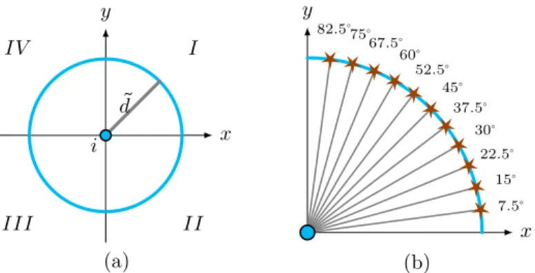
Initial Anchors have their pre-known accurate positions. They are either equipped with GPS or manually predetermined their exact positions. Each node is assumed to be capable of generating a distance estimate to any of its one-hop neighbors. However, nodes are only required to estimate ranges between its location and the anchor nodes. Typically, ranging estimates are performed by one of the four basic techniques. Initially, the algorithm starts by anchor nodes transmitting their own locations to their one hop neighbors. Each node that receives 3 or more anchor locations will start the localization process. Each node selects an anchor node at random to act as a base. The node’s estimated position lies on a circle centered at the base anchor node’s location with a radius
̃
𝑑 which is the estimated range to the node being localized as shown in Fig. 1(a). The challenge arises in determining which point on this circle is the estimated position and in which quadrant this point exist. Thus, an elimination process is proposed and employed as in the next sub-section. 3.2. TALS: basic elimination process
First, the basic simple, low cost and efficient TALS elimination process is described. Second, an additional enhancement and optimization in term of computation cost and complexity while conserving the accuracy level is introduced.
First of all, the circle is divided into points as shown in Fig. 1(b), where each point could be a potential estimate and we will refer to it as an estimate point. The division is done uniformly
𝑥 𝑦 ̃ 𝑑 𝑖 𝐼𝑉 𝐼𝐼𝐼 𝐼𝐼 𝐼 (a) 𝑥 𝑦 7.5∘ 15∘ 22.5∘ 30∘ 37.5∘ 45∘ 52.5∘ 60∘ 67.5∘ 75∘ 82.5∘ (b)
Figure 1: TALS generation of estimate points
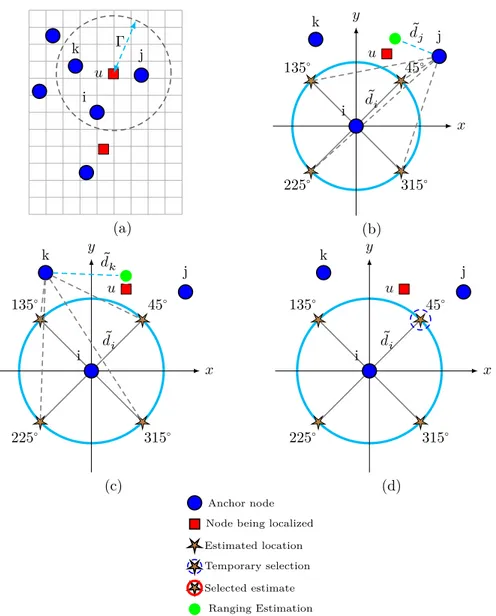
across all quadrants of the circle where only the division of quadrant 𝐼 is shown in Fig. 1(b). The angle degree for which the circle is divided is a design parameter that will be discussed in Sec. 4.2. To choose which point on this circle is the best estimate and eliminate the others candidate points, additional anchor nodes aid in the localization process. We define 𝔸 as the set of these additional anchor nodes. The elimination or the selection is done by comparing the squared estimated range of the node being localized to the squared distance from the additional anchor nodes to the points on the circle through multiple iterations. The elimination process starts by choosing which quadrant the estimate lies on. As shown in Fig. 2(a), consider the base anchor node 𝑖 and two other anchor nodes 𝑙 ∈ 𝔸 = {𝑗, 𝑘}. The algorithm starts initially by selecting four
points which lie on the circle of node 𝑖 at 45∘ from the x-axis as shown in Fig. 2(b,c).
The coordinates of the first estimate point in quadrant 𝐼 can be calculated using the following equations:
̃𝑥
45𝐼= 𝑥𝑖+ ̃𝑑𝑖𝑐𝑜𝑠𝛼, 𝑤ℎ𝑒𝑟𝑒 𝛼 = 45 (1)
̃𝑦
45𝐼= 𝑦𝑖+ ̃𝑑𝑖𝑠𝑖𝑛𝛼, 𝑤ℎ𝑒𝑟𝑒 𝛼 = 45; (2)
The three other estimate points that lie on the other three quadrants can be populated using the trigonometric properties:
̃𝑥 45𝐼𝐼= ̃𝑥45𝐼 , 45𝐼𝐼̃𝑦 = − ̃𝑦45𝐼 (3) ̃𝑥 45𝐼𝐼𝐼= − ̃𝑥45𝐼 , 45𝐼𝐼𝐼̃𝑦 = − ̃𝑦45𝐼 (4) ̃𝑥 45𝐼𝑉 = − ̃𝑥45𝐼 , 45𝐼𝑉̃𝑦 = ̃𝑦45𝐼 (5)
But as each sensor to be localized will take a basic anchor as the reference for its measurements, we need to adapt the previous equations as below:
̃𝑥 45𝐼𝐼 = ̃𝑥45𝐼 (6) ̃𝑥 45𝐼𝐼𝐼 = ̃𝑥45𝐼𝑉 = 𝑥𝑖− ̃𝑑𝑖𝑐𝑜𝑠𝛼 (7) ̃𝑦 45𝐼𝑉 = ̃𝑦45𝐼 (8) ̃𝑦 45𝐼𝐼 = ̃𝑦45𝐼𝐼𝐼= 𝑦𝑖− ̃𝑑𝑖𝑠𝑖𝑛𝛼 (9)
The node will compute (in the basic TALS) the squared distance from anchor 𝑗 and 𝑘 to the 4 points using the following equations (see Fig. 2(b,c)):
̃ 𝑑2 𝑗45𝑚 = (𝑥𝑗− 𝑥45𝑚)2+ (𝑦𝑗− 𝑦45𝑚)2 (10) ̃ 𝑑2 𝑘45𝑚= (𝑥𝑘− 𝑥45𝑚)2+ (𝑦𝑘− 𝑦45𝑚)2 (11)
The above values are compared against the estimated ranges ̃𝑑2
𝑗 and ̃𝑑2𝑘respectively by taking the
absolute difference as follow:
𝜏𝑚= | ̃𝑑2
𝑘− ̃𝑑𝑘45𝑚2 | + | ̃𝑑𝑗2− ̃𝑑2𝑗45𝑚| (12)
for m=I, II, III and IV, the name of a quadrant.
The point that has the lowest residue 𝜏 resulting from taking the sum of absolute differences is the point that is the nearest to the node and hence the quadrant is selected as shown in Fig. 2(d). This is due to the fact that for two-dimensional localization, we need usually three anchor nodes (three range measurements from known positions). Each range can be represented as the radius of a circle, with the anchor node situated at the center. Without measurement noise, the three circles would intersect at exactly one point, the location of the target node. Note that we do not solve a linear system of equations and we do not use square root functions.
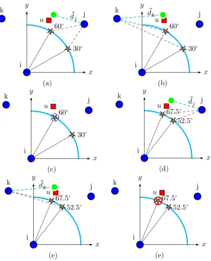
The reason why the squared distance is used in (10), (11) and (12) lies in the fact that square root functions are expensive in terms of computational complexity. In this way, these functions are eliminated and are substituted for them by squared functions that improves the performance without reducing the accuracy. As shown in Fig. 3, the second iteration of the elimination process starts by selecting two new estimate points on the circumference of the selected quadrant, e.g.
quadrant I in this example, located at ±15∘ to/from the first selected point that was lying on 45∘
in our example. That is, the two estimate points lie on the circle of node 𝑖 at 30∘ and 60∘ from
the x-axis as shown in Fig. 3. The coordinates of these two estimate points are calculated using equations (1) and (2) by substituting for 𝛼 by 30° and 60°. The squared distance to these two points are then computed using the following equations.
̃ 𝑑2 𝑎30 = (𝑥𝑎− 𝑥30)2+ (𝑦𝑎− 𝑦30)2, ∀𝑎 ∈ 𝔸 (13) ̃ 𝑑2 𝑎60 = (𝑥𝑎− 𝑥60)2+ (𝑦𝑎− 𝑦60)2, ∀𝑎 ∈ 𝔸 (14)
Subscript a in equations (13) and (14) refers to the anchor node aiding in the localization process. The computed values are again compared against the estimated range where the point with the lowest residual 𝜏 is selected. If at any time the residual 𝜏 is smaller or equal to the threshold 𝜉, the elimination process stops and the point with the lowest residual is selected as the final estimate. The process continues iteratively in a binary-search like manner until the threshold condition is satisfied. For an example, if point 60° is selected and the threshold condition is not met, the third elimination phase selects the two points (52.5° and 67.5°) such that the comparison will be between them as shown in Fig. 3(d,e,f). Therefore, in any new iteration (𝑖), the selection of the
two estimate points (𝑝𝑖1 and 𝑝𝑖2) is done based on the nearest estimate point computed in the
previous iteration (𝑝𝑖−1) using equation (15):
𝑝𝑖1= 𝑝𝑖−1+ 15∘
2𝑖−2
𝑝𝑖2= 𝑝𝑖−1− 15∘
2𝑖−2 (15)
where 𝑖 ≥ 2 stands for the iteration number of the elimination process, and the second term of
the right sides represents the degree of divisions so-called 𝛿𝑖 = 15∘
2𝑖−2 that is the smallest angle
with which the iterative division of the circle of the base anchor node is achieved. The algorithm stops when the threshold condition is met or when the divisions reach 0° or 90°. The effect of the parameter 𝛿 will be discussed in Sec. 4.2.
3.3. Optimization for the elimination process using a novel modified Manhattan distance
Several distance measurement techniques can be applied to measure the distance between two points (i.e. estimate and anchor nodes). One of the most popular is Minkowski distance that is expressed in Eq. (16). Given two vectors 𝑢 and 𝑣 of the same length 𝑁 ≥ 1, Minkowski distance is computed as follows:
k j 𝑢 i Γ (a) 𝑥 𝑦 45∘ 135∘ 225∘ 315∘ k j 𝑢 ̃ 𝑑𝑖 ̃ 𝑑𝑗 i (b) 𝑥 𝑦 45∘ 135∘ 225∘ 315∘ k j 𝑢 ̃ 𝑑𝑖 i ̃ 𝑑𝑘 (c) 𝑥 𝑦 45∘ 135∘ 225∘ 315∘ k j 𝑢 ̃ 𝑑𝑖 i (d) Anchor node Node being localized Estimated location Temporary selection Selected estimate
Ranging Estimation
Figure 2: TALS generation of estimate points.
𝑑𝑖𝑠𝑡(𝑢, 𝑣) = 𝑀𝑖𝑛𝑘𝑜𝑤𝑠𝑘𝑖𝑝(𝑢, 𝑣) =𝑝 𝑁
𝑖=1
𝑑(𝑢𝑖, 𝑣𝑖)𝑝=𝑝 𝑁 𝑖=1
|𝑢𝑖− 𝑣𝑖|𝑝 (16)
where 𝑝 is the order of Minkowski distance. Manhattan or city block distance is a special case of Minkowski when 𝑝 = 1 and when 𝑝=2, the Minkowski distance is so-called Euclidean distance. In fact, the Euclidean distance gives an accurate measure because it represents the length of the line segment connecting two different points. However, the cost is relatively high because of the use of the root square and the sum of squares as we will see in Sec. 5.9.
In this section, a novel distance measurement technique is proposed to compute the residue 𝜏 that indicates the nearest estimate point in each iteration to the real position of the node being localized. The novel Modified Manhattan Distance technique (MM) replaces the Euclidean distance employed in TALS through all the iterations of the elimination process. Our aim is to conserve the accuracy while reducing the cost and the complexity as explained in Sec. 3.4 and Sec. 5.
In fact, 𝜏 in (12) was based on equations (10), (11), (13), and (14) that use the Pythagorean theorem; it requires the square function. The new comparison will be given through the following
𝑥 𝑦 30∘ 60∘ k j 𝑢 i ̃ 𝑑𝑗 (a) 𝑥 𝑦 30∘ 60∘ k j 𝑢 i ̃ 𝑑𝑘 (b) 𝑥 𝑦 30∘ 60∘ k j 𝑢 i (c) 𝑥 𝑦 52.5∘ 67.5∘ k j 𝑢 i ̃ 𝑑𝑗 (d) 𝑥 𝑦 52.5∘ 67.5∘ k j 𝑢 i ̃ 𝑑𝑘 (e) 𝑥 𝑦 52.5∘ 67.5∘ k j 𝑢 i (e)
Figure 3: Example of the second iteration phase in TALS elimination process.
equation
𝜏𝑝=
𝑗∈𝔸
| ̃𝑑𝑗− ̃𝑑𝑗𝑝| , (17)
where 𝑝 represents an estimate point in a given iteration, ̃𝑑𝑗 denotes the estimated range of the
node being localized by the anchor 𝑗 ∈ 𝔸, and ̃𝑑𝑗𝑝 denotes the estimated distance between anchor
node 𝑗 and an estimate point 𝑝. This later distance will be computed using a modified Manhattan instead of the squared Euclidean distance, that was utilized in the basic elimination process, as shown in Eq. (18).
̃
𝑑𝑗𝑝= ̃𝑑𝑋𝑗𝑝+ ̃𝑑𝑌𝑗𝑝+ 𝜃| ̃𝑑𝑋𝑗𝑝− ̃𝑑𝑌𝑗𝑝| (18)
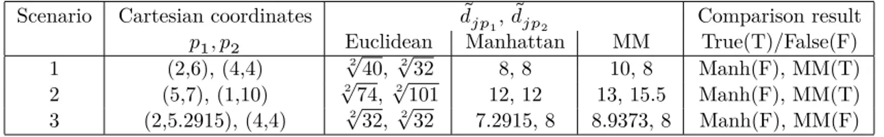
where ̃𝑑𝑋𝑗𝑝 = |𝑥𝑗−𝑥𝑝| and ̃𝑑𝑌𝑗𝑝 = |𝑦𝑗−𝑦𝑝| and 𝜃 is a real constant. The first and the second terms in (18) represent Manhattan distance and the third term represents a corrective factor that will ensure a higher accuracy level of the comparison. Manhattan sometimes gives wrong estimations as shown in the following examples where our modified Manhattan gives more accurate comparison results. The next sub-sections prove that a very good value 𝜃 can be set to, in terms of accuracy and complexity, 0.5.
In order to highlight the advantage of the proposed MM over Manhattan, in term of accuracy,
three different scenarios of the 3 nodes location (one anchor 𝑗 ∈ 𝔸 and two estimate points 𝑝1and
𝑝2) are considered and the Manhattan, MM, and Euclidean distances are applied to determine
Table 1: Scenarios settings and results
Scenario Cartesian coordinates 𝑑𝑗𝑝̃
1, ̃𝑑𝑗𝑝2 Comparison result
𝑝1, 𝑝2 Euclidean Manhattan MM True(T)/False(F)
1 (2,6), (4,4) √240, √232 8, 8 10, 8 Manh(F), MM(T)
2 (5,7), (1,10) √274, √2101 12, 12 13, 15.5 Manh(F), MM(T)
3 (2,5.2915), (4,4) √232, √232 7.2915, 8 8.9373, 8 Manh(F), MM(F)
anchor 𝑗 to be (0,0) and that the value of 𝜃 = 0.5 in (18) for the MM distance. Table 1 resumes the three scenarios settings and results.
In the first scenario, we consider the Cartesian coordinates of the estimate points to be (2,6)
and (4,4) respectively. The estimate point 𝑝2 is closer than 𝑝1 to the anchor node 𝑗 because
the Euclidean distances between 𝑗 from one side and 𝑝1 and 𝑝2 from the other side are √24 + 36
and √216 + 16 respectively. Using the Manhattan formula, these distances are equivalent because
dist(j,𝑝1) = 2+6 = 8 and dist(j,𝑝2) = 4+4 = 8. Therefore, Manhattan gives a wrong comparison
result in this scenario. However, our formula of MM (18) gives the right result because ̃𝑑𝑗𝑝1 =
2 + 6 +4
2 = 10 and ̃𝑑𝑗𝑝2 = 4 + 4 +
0
2 = 8. Let us presume a second scenario where 𝑝1 and 𝑝2 are
(5,7) and (1,10). Here, the estimate point 𝑝1 is closer than 𝑝2 to the anchor node 𝑗 because the
Euclidean distances are √274 and √2101 respectively. Using the Manhattan formula, we find the
opposite result; another wrong estimate. Now, using MM we find that ̃𝑑𝑗𝑝1 = 5 + 7 +2
2 = 13 and
̃
𝑑𝑗𝑝2= 1 + 10 + 9
2 = 15.5, and thus it gives an accurate comparison result.
We show now that MM gives in some particular scenarios wrong results as Manhattan. The frequency of such a wrong result is very low as demonstrated in the next subsection. We consider
𝑝1=(2,5.2915) and 𝑝2=(4,4). The Euclidean distances between 𝑗 from one side and the estimate
points are calculated as √24 + 28 and √216 + 16 respectively. Using the Manhattan formula, the
distances are dist(j,𝑝1) = 2+5.2915 = 7.2915 and dist(j,𝑝2) = 4+4 = 8. Similar to Manhattan in
such a particular scenario, MM cannot capture the true result because ̃𝑑𝑗𝑝1= 2+5.2915+3.2915
2 =
8.9373 and ̃𝑑𝑗𝑝2 = 4 + 4 +0
2 = 8 and thus Manhattan (resp. MM) decides that 𝑝1 (resp. 𝑝2) is
closer than 𝑝2 (resp. 𝑝1) to 𝑗.
In the next subsection, we first evaluate the comparison accuracy of our proposed MM formula as function of 𝜃. We quantify the error frequency made when using MM instead of the Euclidean distance. Second, we compare through simulating the relative error made by MM with respect to that made by Manhattan.
Fortunately , the elimination process does not depend on a single comparison result from one
anchor node. In Equ. (17), 𝜏𝑝depends on the comparison results of at least two anchor nodes. We
demonstrate through simulation in Sec. 5, which addresses the validation and the performance evaluation of the overall OTALS, that the optimized elimination process ensures a very good accuracy with less complexity than the basic process and other localization algorithms found in the literature (to the best of our knowledge).
3.4. Accuracy Evaluation of the Modified Manhattan technique
We will now analytically evaluate the accuracy of our enhanced version of the elimination process using intensive simulation through Matlab that will help to better understand the impact of the wrong result on the localization process.
3.4.1. Analytic analysis
Consider two points 𝐴 = (𝑎, 𝑏) and 𝐵 = (𝑐, 𝑑). We know that 𝐴 is closer (resp. farther) from the origin (0, 0) than 𝐵 if 𝑎2+ 𝑏2< 𝑐2+ 𝑑2 (resp. 𝑎2+ 𝑏2 > 𝑐2+ 𝑑2).
Question: when do we make a mistake if we replace the above criterion by the criterion “𝐴 is closer (resp. farther) from the origin than 𝐵 if 𝑎 + 𝑏 + 𝜃|𝑎 − 𝑏| < 𝑐 + 𝑑 + 𝜃|𝑐 − 𝑑| (resp. 𝑎 + 𝑏 + 𝜃|𝑎 − 𝑏| > 𝑐 + 𝑑 + 𝜃|𝑐 − 𝑑|) with 𝜃 ≥ 0?
−2 −1.75 −1.5 −1.25 −1 −0.75 −0.5 −0.25 0 0.25 0.5 0.75 1 1.25 1.5 1.75 2 0 2 4 6 8 10 12 14 16 18 20 22 24 26 28 30 32 34 35 The θ Parameter
Distances Comparisons Error percentage
Figure 4: Analysis of Accuracy of Modified Manhattan as function of 𝜃.
Define 𝑋 ∶= 𝑎2+ 𝑏2− (𝑐2+ 𝑑2) and 𝑌 ∶= 𝑎 + 𝑏 − (𝑐 + 𝑑).
It is easily seen that 𝑋 < 0, or equivalently 𝐴 is closer than 𝐵 from the origin, if and only if
𝑌 < 𝑎 + 𝑏 + 𝑐 + 𝑑2(𝑎𝑏 − 𝑐𝑑) . (19)
We therefore need to compare the criterion in (19) to the criterion
𝑌 < 𝜃|𝑐 − 𝑑| − 𝜃|𝑎 − 𝑏|. (20)
With (19) and (20) the answer to the question above is easy. If 𝜃|𝑐 − 𝑑| − 𝜃|𝑎 − 𝑏| < 2(𝑎𝑏−𝑐𝑑)
𝑎+𝑏+𝑐+𝑑 then using criterion (20) will give the wrong answer for all
points 𝐴 and 𝐵 such that 𝜃|𝑐 − 𝑑| − 𝜃|𝑎 − 𝑏| < 𝑌 < 2(𝑎𝑏−𝑐𝑑)
𝑎+𝑏+𝑐+𝑑. Similarly, if 𝜃|𝑐 − 𝑑| − 𝜃|𝑎 − 𝑏| > 2(𝑎𝑏−𝑐𝑑)
𝑎+𝑏+𝑐+𝑑 then using criterion (20) will give the wrong answer for all points 𝐴 and 𝐵 such that 2(𝑎𝑏−𝑐𝑑)
𝑎+𝑏+𝑐+𝑑< 𝑌 < 𝜃|𝑐 − 𝑑| − 𝜃|𝑎 − 𝑏|.
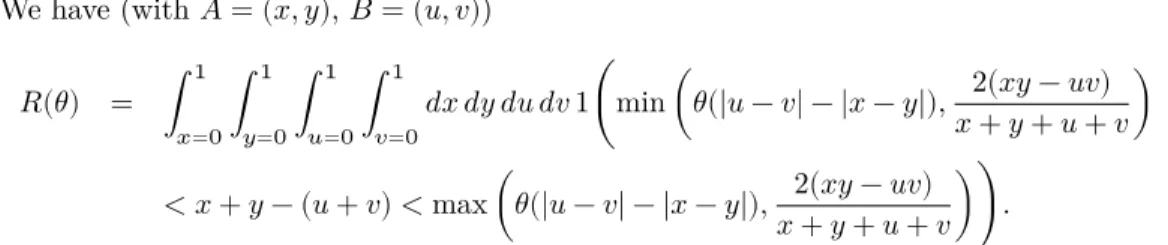
In summary, criterion (20) will give the wrong answer for all points 𝐴 and 𝐵 such that min 𝜃(|𝑐 − 𝑑| − |𝑎 − 𝑏|),𝑎 + 𝑏 + 𝑐 + 𝑑2(𝑎𝑏 − 𝑐𝑑) < 𝑌 < max 𝜃(|𝑐 − 𝑑| − |𝑎 − 𝑏|),𝑎 + 𝑏 + 𝑐 + 𝑑2(𝑎𝑏 − 𝑐𝑑) . Let us now quantify the error that is made when using the criterion (20) instead of the Euclidean distance. To do that, consider a square of size 1 and let us calculate the ratio 𝑅(𝜃) of pair of points in this square for which criterion (20) will return a wrong answer.
We have (with 𝐴 = (𝑥, 𝑦), 𝐵 = (𝑢, 𝑣)) 𝑅(𝜃) = 1 𝑥=0 1 𝑦=0 1 𝑢=0 1 𝑣=0 𝑑𝑥 𝑑𝑦 𝑑𝑢 𝑑𝑣 1min 𝜃(|𝑢 − 𝑣| − |𝑥 − 𝑦|), 2(𝑥𝑦 − 𝑢𝑣) 𝑥 + 𝑦 + 𝑢 + 𝑣 < 𝑥 + 𝑦 − (𝑢 + 𝑣) < max 𝜃(|𝑢 − 𝑣| − |𝑥 − 𝑦|),𝑥 + 𝑦 + 𝑢 + 𝑣2(𝑥𝑦 − 𝑢𝑣) .
Fig. 4 shows the ratio 𝑅(𝜃) for 𝜃 = −2 ∶ 0.1 ∶ 2. We notice that the best value of 𝜃 is equal to 0.4 (It corresponds to 2.0232% of error i.e. the minimum). However, from the practical point of view, setting the value of 𝜃 to 0.5 (the second best value that corresponds to 2.574% of error) allows the engineers as shown in the next subsection to replace the complex computations (roots, square, multiplication , division, etc) by a simple shift process (dividing over two in a binary representation) with a minor additional comparison error. Note that the MM becomes Manhattan when 𝜃 = 0. From Fig. 4 we see that Manhattan gives 6.325% of the wrong results. 3.4.2. Choice of 𝜃’s value
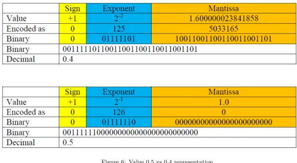
We introduce in this subsection the reason of setting 𝜃 to 0.5 instead of 0.4 since equations (17) and (18) do not give enough evidence of saving additional computational complexity with this setting. Multiplication and division operations require many instruction cycles to be performed. In the absence of a hardware multiplier, like a low profile sensor node, multiplication and division can be performed with shift and add operations. Shift-add-multiplication is the simplest way to perform multiplication (see [? ? ]). It is derived for binary (n-bits x n-bits) integer which can also be used for single precision floating point number with some minor changes. The number of intermediate addition operations for shift-and-add multiplication method is equal to the number of 1’s in the multiplier number. Real numbers are represented by different ways, but the IEEE floating point representation is the most used one. The single precision floating point representation is defined by the IEEE 754 and is represented by 32 bits. These bits are divided into three bit fields: sign bit (1-bit), biased exponent (8-bits), and mantissa (or fraction) (23-bits) as shown in Fig 5.
The positive and negative normalized numbers closest to zero are ±2−126 ≈ ±1.17949𝑥10−38.
The finite positive and finite negative numbers furthest from zero are: ±(1 − 2 − 24)𝑥2128 ≈
±3.40282𝑥1038. The sign is stored in bit 32. The exponent can be computed from bits 24-31 by
subtracting 127. The mantissa (also known as significant or fraction) is stored in bits 1-23.
Figure 5: Number representation
Figure 6 illustrates the representation of the values 0.5 and 0.4 using the IEEE 754 floating point representation. It is clear from the representation that multiplying by 0.5 only needs a one shift operation compared to multiplying by 0.4 which needs a larger number of shift operations and add operations and, as a result, a larger power consumption. Actually, there are 12 ones in the representation of the mantissa field for the value 0.4, which means 12 add and shift operations are needed, if a simple multiplication algorithm is employed.
3.4.3. Evaluation of MM through Simulation
We now evaluate the accuracy of our enhanced version of the elimination process using inten-sive simulation through Matlab while considering 𝜃 = 0.5. We assume a square area of dimensions 31x31 measurement unit, e.g. 𝑚. We take 10218313 random possible locations of two estimate points around an anchor node. The total numbers of the wrong estimations using Manhattan and Modified Manhattan are 623320 and 194704 respectively. The relative errors for both techniques are 6.1% and 1.91% respectively. To understand the reason of the wrong estimations, we first
Figure 6: Value 0.5 vs 0.4 representation
maintain two arrays of length equal to the number of wrong estimations using the Manhattan method and the Modified Manhattan method respectively. The value of each element in both arrays correspond to the absolute difference between the straight-line distances of the two esti-mate points to the anchor node. Then, we draw the histogram of those two arrays that shows the error frequency of the estimation results in both Manhattan and our modified Manhattan techniques with respect to differences between the straight-line distances of the estimate points as demonstrated in Fig. 7. We notice from the figure that the high error frequency occurs when the difference between the straight-line distances of the estimate points to the anchor node is equal to zero, and then to one and two (the estimate points are at the same distance or close to be at the same distance from the anchor node). In fact, with very high probability, this happen in the last iteration phases of the elimination process where the estimate nodes become so close to the right position, and then even if a wrong estimation is made by MM, a very close position is already found. However, and this is a very important remark, when both estimate points are from one distance of one anchor node, they will be with high probability at different straight-line distances from the second anchor nodes that participate in the elimination process. Therefor, the error fre-quency of the elimination process that depends on the comparison results from at least two Anchor nodes as shown in Eq. (17) will be highly reduced as we will see in Sec. 5. We conclude from the analysis and simulation results that the modified Manhattan is very efficient for hardware of embedded system environment of WSN. This conclusion will be justified and confirmed through accuracy comparison with other previous works and through complexity analysis in Section Sec. 5. It saves more than the 50% of the basic operations number (i.e. binary add operation) used in the calculation of the distance between two nodes similar to Manhattan. In addition, it is more accurate than the Manhattan distance and less complex than the Euclidean technique and other methods appeared in the literature, that require basically solving a linear system of equations via least square or its variant or require a high relative number of iterations for the distributed formulation in previous works.
3.5. Selection of base anchor
In this section, we show how a base anchor is selected. Initially, the ordinary node 𝑢 that is not localized yet finds 𝑛 surroundings anchors within its transmission range Γ as in Fig. 2(a). Only if (𝑛 > 2), node 𝑢 starts the localization process by selecting one of its surroundings anchors as its base. The highest priority of neighbor anchors to be a base will be given to the fixed anchors. Now, we define two methods to select a base anchor and describe each one in details. The two
0 5 10 15 0 0.5 1 1.5 2 2.5x 10 5
Manhattan Error Frequency (B)
Direct Distance between the estimate points
0 1 2 3 4 5 6 7 8 x 10⁴
Modified Manhattan Error Frequency (R)
Figure 7: Comparison between Modified Manhattan and Manhattan distances.
methods differ in the computational complexity and storage space.
Method 1: Selecting one base anchor randomly from all neighbor anchors. Fig. 2 shows an example in which node 𝑢 chooses anchor node 𝑖 to be its base anchor and then starts to compare
the estimated positions on the base anchor circle circumference with radius ̃𝑑𝑖 to the distance
from the other anchor nodes 𝑗 and 𝑘. Random selection may be useful for wireless networks with nodes having low computational power. However, it may result in significant errors in selecting the quadrant at the elimination process as we will see in Sec. 4.1.
Method 2: Repeat method one with each anchor, considering one anchor as a base at a time, then selecting the one that leads to the lowest residual. This means that the selection process repeats for all anchor nodes where the next anchor will act as a base and the remaining anchors will aid in the localization process. This way, for each anchor node received by the localizing node, an estimate will be produced. This redundancy will be of a great benefit where fusion techniques can be employed to combine the estimates into an accurate location as shown in Sec. 3.6.
Note that in case the sensor is surrounded by more than three anchors we can consider taking 𝑟 anchors at a time where (3 ≤ 𝑟 ≤ 𝑛), where 𝑛 is the maximum number of anchor nodes in the
range of the given sensor. In this case the total number of the combinations is (∑𝑛
𝑖=3 𝑛𝐶𝑖). a
key issue to be considered is the simplicity of the localization algorithm because it is crucial for implementation and efficiency purposes.
3.6. Data Fusion Technique and Accuracy Enhancement
As shown in Sec. 3.5, TALS repeats the location selection procedure for each anchor node by setting them as base nodes one at a time. Thus, for each anchor node location received, an estimate for the node being localized is calculated. This redundancy enhances the quality of the estimates and eliminates diverging measurements to a great extent. Since TALS computes the locations of the nodes iteratively, weights can be assigned to add confidence to anchor nodes.
The first step in TALS algorithm starts by anchor nodes broadcasting their locations. Each node that receives more than three anchor nodes’ location can start the estimation process of its own location. These nodes are upgraded to become virtual anchor node status and broadcast their locations to neighboring nodes and the localization process continues until all nodes are localized. Confidence is given according to two parameters: the number of fixed or virtual anchor nodes and the distance to the node being localized. Higher confidence is given for fixed anchor nodes since
they have accurate positions. Thus, given the set of fixed anchors 𝐹𝑎𝑛𝑐ℎ𝑜𝑟𝑠 and the set of virtual
anchors 𝑉𝑎𝑛𝑐ℎ𝑜𝑟𝑠, the probabilistic weight is given according to equation (21) where 𝜙 represents
an empty set. 𝑤𝑎(𝑖) = ⎧ ⎨ ⎩ 0.75 |𝐹𝑎𝑛𝑐ℎ𝑜𝑟𝑠| , if{i𝐹𝑎𝑛𝑐ℎ𝑜𝑟𝑠}&{𝑉𝑎𝑛𝑐ℎ𝑜𝑟𝑠≠ 𝜙} 1 |𝐹𝑎𝑛𝑐ℎ𝑜𝑟𝑠| , if{i𝐹𝑎𝑛𝑐ℎ𝑜𝑟𝑠}&{𝑉𝑎𝑛𝑐ℎ𝑜𝑟𝑠= 𝜙} 0.25 |𝑉𝑎𝑛𝑐ℎ𝑜𝑟𝑠| , if{i𝑉𝑎𝑛𝑐ℎ𝑜𝑟𝑠}&{𝐹𝑎𝑛𝑐ℎ𝑜𝑟𝑠≠ 𝜙} 1 |𝑉𝑎𝑛𝑐ℎ𝑜𝑟𝑠| , if{i𝑉𝑎𝑛𝑐ℎ𝑜𝑟𝑠}&{𝐹𝑎𝑛𝑐ℎ𝑜𝑟𝑠= 𝜙} (21)
As shown in equation (21), each anchor node belonging to the localizing node’s list of anchor
nodes is assigned a probabilistic weight 𝑤𝑎according to its status. The value 0.75 in the equation
means multiply by 3 and divide by 4, which is 2 shift operations in binary representation and not a real division. Thus, we keep the simplicity of the low computation cost of TALS. In fact, if the anchor node’s list contains only fixed or virtual anchor nodes, each anchor node will receive equal weight assignment. On the other hand, if the anchor list contains mixed fixed and virtual anchors, fixed anchor nodes are assigned higher weights than virtual anchors since the latter can have inaccuracies about their estimated positions. Moreover, low estimated ranges from the base anchor node to the node being localized should be assigned high weights since low ranges minimize errors. In this context, given the distance from the base anchor node to the node being localized
𝑑𝑖 and the maximum transmission range Γ, the probabilistic weight 𝑤𝑑 is assigned according
to equation (22). Consequently, each estimate computed from each anchor node is assigned the
normalized weight 𝑤𝑑𝑁 as shown in equation (23).
𝑤𝑑(𝑖) = 1 −𝑑𝑖
𝛾 (22)
𝑤𝑑𝑁(𝑖) = 𝑤𝑑(𝑖)
∑𝑛_𝑎𝑛𝑐ℎ𝑜𝑟𝑠𝑗=1 𝑤𝑑(𝑗) (23)
Since 𝑤𝑑𝑁 and 𝑤𝑎 are independent, their joint probability distribution is given by (24). The
final weight assigned for each estimate generated by an anchor node is given by (25). The final estimate is given by equation (26).
𝑃 (𝑤𝑑𝑁(𝑖), 𝑤𝑎(𝑖)) = 𝑤𝑑𝑁(𝑖) × 𝑤𝑎(𝑖) (24) 𝑤(𝑖) = 𝑃 (𝑤𝑑𝑁(𝑖), 𝑤𝑎(𝑖)) ∑𝑛_𝑎𝑛𝑐ℎ𝑜𝑟𝑠𝑗=1 𝑃 (𝑤𝑑𝑁(𝑗), 𝑤𝑎(𝑗)) (25) ( ̃𝑥, ̃𝑦) =𝑛_𝑎𝑛𝑐ℎ𝑜𝑟𝑠 𝑖=1 𝑤(𝑖) × ( ̃𝑥𝑖, ̃𝑦𝑖) (26)
4. Analysis
In this section, we analyzing the impacts of different parameters of the optimized TALS on the localization process. Additional parameters that are difficult to formulate analytically are studied using simulation.
4.1. Accuracy of Quadrant Selection
As stated before the elimination process starts by choosing which quadrant the estimate lies in. The algorithm starts initially by selecting four points which lie on the circle of node 𝑖 at 45° from the x-axis. The point that has the lowest residue resulting from taking the sum of absolute differences is the point that is the nearest to the node, hence the quadrant is selected. Next, we show by example that this step may lead to the wrong quadrant when anchors nodes roughly lie on a straight line. This problem is known in the literature as the collinear anchor problem (see [? ], [? ]). However, by deployment of Method 2 discussed in the previous section or applying a data fusion technique (presented in Sec. 3.6), we can easily overcome this possible wrong estimation. 4.1.1. Example of wrong estimation
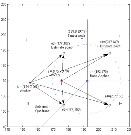
Figure 8 gives an example for the output of TALS/OTALS algorithm. In the figure, there are three Anchors 𝑖 = (192, 170); 𝑘 = (154.7, 169); 𝑗 = (175.2, 170) and a sensor node to be localized at (188.9, 197.7). The figure shows an example of the wrong estimation of the Quadrant when the anchor 𝑖 is selected to be the base anchor in the elimination process. The sensor node actually lies in quadrant II and OTALS wrongly evaluates it to lie in quadrant III. In other words, in the first iteration, instead of selecting the estimate point 𝑒2, the algorithm selects 𝑒3 as it is the point
that has the lowest residue 𝜏 computed from (17). 𝜏𝑒3= (|177-154.7|)+(|153-169|)+0.5*(|22.3-16|)
+ (|177-175.2|)+(|153-170|)+0.5*(|1.8-17|) = 41.45 + 26.4 = 67.85 is the lowest value, then 𝜏𝑒2
= (|177-154.7|)+(|187-169|)+0.5*(|22.3-18|) + (|177-175.2|)+(|187-170|)+0.5*(|1.8-17|) = 42.45 + 26.4 = 68.85 , then 𝜏𝑒4 and the last value 𝜏𝑒1.
4.2. Analysis of the effect of Degree of Divisions and Threshold Selection
The degree of divisions 𝛿 is defined as the smallest angle with which the iterative division of the circle of the base anchor node is achieved as shown in Eq (15). For example, the case shown in Fig. 1(b) has the smallest angle 𝛿 set to 7.5°. The number of estimate points 𝜅 is given by 𝜅 =
360
𝛿 . The selection of 𝛿 depends on an acceptable estimation error which is an application-based
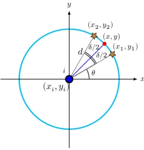
parameter. Finer granularity of 𝛿 will yield lower error which comes at the cost of increasing the iterative computations because the number of the elimination phases increase. Therefore, 𝛿 is related with the threshold 𝜉. It was stated in Sec. 3.1 that if at any time the residual 𝜏 is smaller or equal to the threshold 𝜉, the elimination process stops and the point with the lowest residual is selected as the final estimate. Thus, the selection of the threshold 𝜉 depends on two parameters: the degree of division 𝛿 and the maximum transmission range Γ. Higher ranges will yield larger radii which translate into bigger pores between the estimated points. The threshold selection is bounded by equation (27) which is given by Theorem 1 that is presented and proofed by Merhi et. al. in [? ].
Theorem 1. Given no errors are introduced on the ranging measurements between the localizing node and the anchor node in a one hop scenario, the maximum error is bounded by equation (27):
𝜉𝑚𝑎𝑥= Γ2(1 − 𝑐𝑜𝑠(𝛿2)) (27)
Figure 8: Example of wrong quadrant estimation
4.3. TALS Refinement
There is a trade-off between achieving higher accuracy of the localization algorithm, by reducing the degree of division 𝛿 and reducing the computational complexity. In fact, the sine and cosine operations used to determine the estimate points shown in equations (1) and (2) have non negligible computation cost. This section illustrates how computational complexity was decreased by offline pre-calculating the values of the sine and cosine and storing them in the memory of the sensor node. In addition, the trigonometric properties presented in equations (28) and (29) are utilized to further optimize the required number of entries to store the sine and cosine values.
Since the division points on the circle are static and the TALS algorithm tries to select the next point to consider and test for, the sine and cosine values for these points can be stored in a lookup table. However as 𝛿 decreases, the number of entries needed to store the sine and cosine values increases, and as a result the size of the look up table increases. Given the the fact that the four quadrants act like mirrors to each other, only 1/4 of the table entries need to be stored. In addition, equations (28) and (29) show that only one entry is needed for the sine or cosine functions. Thus, we need 0.25*360/𝛿. If 𝛿 = 7.5, we need only 12 entries compared to 96 (12 * 4 quadrants * 2 sine and cosine values) entries if the trigonometric properties are not taken into consideration. In fact the optimization can go further using the trigonometric laws and the total lookup table size for each sine and cosine value is given by 45/𝛿+2, which yield a, 87% saving in the required storage for 𝛿 = 7.5.
𝑥 𝑦 (𝑥, 𝑦) (𝑥2, 𝑦2) (𝑥1, 𝑦1)
(𝑥
𝑖, 𝑦
𝑖)
𝜃 𝑖 𝛿/2 𝛿/2𝑑
Figure 9: Maximum error in a one-hop scenario.
𝑠𝑖𝑛(𝛼) = 𝑐𝑜𝑠(90 − 𝛼) (29)
5. Validation and Performance Evaluation of the optimized TALS
The performance of the Optimized TALS (OTALS) localization system in term of accuracy is evaluated through a simulation study and a quantitative comparison with other known algorithms for the same localization task (push-pull estimator PPE [? ], Least-Squares localization algorithm based on the Levenberg–Marquardt methodology LM as discussed in [? ], and Distributed Spatially Constrained Localization-Local DSCL algorithm [? ]) using the set of real network measurements reported in [? ]. In addition, The computational complexity analysis of the proposed scheme shows the cost efficiency of OTALS. All the simulation scenarios are carried out in MATLAB (The source code is available in [? ] for academic use). The next subsection presents the simulation environment, the parameters settings, and the performance metrics.
5.1. Simulation settings
In our simulation, we assumed two different squares deployment areas with sides length 100x100 and 500x500 grid unit. We used a standard uniform pseudo-random generator to distribute the sensors in the deployment area. Note that there are no restrictions for the places where a sensor can be placed, it can be placed at any grid point. We run several simulation experiments using different sensor densities (from 80 up to 250 sensors) in the deployment areas and different percentage of the anchor nodes (from 5% up to 80%). In order to mitigate the randomness, we repeat each experiment 100 times and report the average of the outputs. We stop the simulation when all the nodes having enough neighbor anchors (or virtual anchor) nodes are localized. We consider scenarios with and without noisy range measurements. We assume in some scenarios nodes with homogeneous transmission range of 20, 25 and 35 distance units and in other scenarios with heterogeneous transmission ranges, randomly assigned between 5 and 35 distance units. The localization error is the average of the Euclidean distance between the actual and the estimated positions of sensors. Mathematically, as expressed in (30)
𝐴𝑣𝑔.𝐸𝑟𝑟𝑜𝑟 = ∑
𝑢
𝑖=1( ̃𝑥𝑖− 𝑥𝑖)2+ ( ̃𝑦𝑖− 𝑦𝑖)2
𝑢 (30)
where 𝑢 is the number of ordinary nodes, ( ̃𝑥𝑖, ̃𝑦𝑖) is the estimated node position, and (𝑥𝑖, 𝑦𝑖) is the actual node position. In all experiments and for any base node 𝑖, the degree of division 𝛿 is set to 7.5°.
5.2. Validation of OTALS
We will validate the global functionality of OTALS and show how it gives very accurate re-sults in different scenarios. A comparison between OTALS, TALS and other different previously published algorithms is provided and a complexity analysis is introduced. The accuracy and the performance evaluation of the optimized TALS with respect to the different system parameters are addressed.
Figure 10 shows an example of regular WSN topology in a deployment area of 500x500 units and 250 sensors. The number of anchors is 50 nodes (20%). The transmission range is randomly distributed between (10 and 35 unites) and we do not consider noise in the transmission mea-surements. The figure shows the comparison result between the exact and estimated locations of sensors. We can notice how good the accuracy of OTALS is (96% of the estimated locations overlap the exact ones). For this scenario, we calculated the absolute estimation error vector as the difference between the distance of the exact position of unlocalized nodes to the center and the distance of the estimated position to the center. We reported the mean value of the error and the variance and we depict in Fig. 11 the histogram of this metric. The mean value of the error is 0.3162 measurement unit and the variance is 4.7349 measurement unit. It is clear from the histogram that 246 sensors out of 250 are localized with absolute estimation error less than 2.5 measurement unit.
Figure 12 shows a different scenario where the grid is 100X100 units and the density is 80 sensors with only 10% Anchors (8 Anchors) with transmission range between (5 and 35 unites). The unlocalized nodes that have enough anchor neighbors (3 at least), will become later virtual Anchors and will aid in the localization process of the others. It is clear that OTALS is a very good algorithm even with small number of initial Anchors.
In the following sections, we carefully examine the effects of different parameters on the overall performance.
5.3. Impact of anchor density
The anchor ratio is one of the most important factors affecting the localization accuracy. Thus, we report accuracy and performance results with a varying number of anchor nodes. Since the ratio of the anchor nodes is controlled by the fixed number of sensor nodes deployed in the sensor field, the number of normal nodes decreases if the number of anchor nodes is increased. In this case we are more interested in the performance when the anchor ratio is small because in a practical system the number of anchor nodes will be much lower than the number of unlocalized nodes. Figure 13 shows that different anchor ratios will influence the location errors. One can see that with the same node density at the same deployment area, when the percentage of initial anchors is increased from 20% to 30%, the average localization errors decrease significantly. Our algorithm performs well as it manages to produce less error, even without large numbers of fixed anchors as clearly shown in Fig. 12.
5.4. Impact of node density
Our second goal from the simulation is to determine the effect of node density on the localization success ratio and on the average of the localization error. For this experiment, we gradually increase the number of nodes from 80 to 220 in the same deployment square areas. As the number of nodes grows, the node density increases, and the number of virtual anchors increases too. As depicted in Fig. 13(a), we find that as we increase the node density, the localization success ratio gets higher as expected. The question that has been answered here is: What is a good initial fixed anchor ratio to achieve certain accuracy level or localization error?. We conclude that nodes benefit from more neighbors and redundancy. Also, that the error propagation of ordinary nodes becoming derived anchors and aiding other nodes in the localization process is within an acceptable range.
5.5. Localization under noisy distance measurements
In this simulation, the noisy range measurements are generated randomly and the distance error variation has a maximum of 5% of the actual distance between nodes. As shown in Fig. 13(b), the localization error is plotted against the ranging measurements error. With the increase of ranging errors, the localization accuracy is affected. However, with small noise range measurements, the influence is still negligible in the proposed optimized TALS contradicting many known localization systems.
5.6. Impact of transmission range
Figure 14 shows that OTALS performs better at high transmission ranges where the unlocalized nodes benefiting from more fixed and virtual anchors. The percentage of fixed anchor nodes is kept fixed at 20% and the transmission range in the simulation varies between 10–50 units. Note that for the smallest transmission range available (10 units), the average error is small because many nodes will not be localized (less than three anchor or virtual neighbor nodes are found) and has no error to be calculated. With larger transmission range, more nodes (and potentially all) will be localized and their errors will start to be calculated. However, as we increase the transmission range (above the value that permits most nodes to be localized), average localization error decreases. In addition, with the increase of the network density, the error decreases in a slow rate.
5.7. Localization of non-convex networks
Finally, we evaluate OTALS in non-convex networks. Figure 15 illustrates two instances. The sensors are randomly deployed in a H-shaped, and a C-shaped regions, respectively. We repeat the simulations and the results are consistent to show the applicability and efficiency of OTALS in localization of non-convex networks as shown in Fig. 16.
5.8. Comparison with other previous algorithms
In this subsection, we evaluate the accuracy of OTALS using the set of real network measure-ments reported in [? ]. This data set has been used in other works [? ], [? ], and [? ], making it a good comparison reference. The data set presents a fully connected network (all devices are in range of all other devices) of 40 sensors randomly deployed in an office environment within a 14 by 13 area. Also, this WSN scenario uses four anchors located intentionally in the corners with the goal of increasing their quality [? ] and avoiding the collinear anchor problem (see [? ], [? ]). The data set consists of ToA and RSS measurements. However, we will consider only the case of range-based on ToA measurements. ToA measurement errors are Gaussian with a standard deviation around 1.84 m.
For comparison, we include localization results from the push-pull estimator PPE [? ], the Least-Squares localization algorithm based on the Levenberg–Marquardt methodology LM as dis-cussed in [? ], the Distributed Spatially Constrained Localization-Local DSCL algorithm [? ] and the basic TALS [? ]. All these algorithms will be tested using similar procedures. As explained
in [? ? ], a set of initial positions 𝐿0 is required for the three first algorithms (PPE, LM, and
DSCL). Each sensor can compute an initial position using an anchor-based localization scheme similar to the ones reported in [? ]. Note that this initial phase is not required for TALS and OTALS, and thus our algorithm economizes energy consumption of this step which is very ex-pensive as explained in [? ] and shown in the next subsection. Additional difference between our algorithm and the three algorithms mentioned above is that each sensor must know positions and range measurements to at least three non-collinear anchors and that at the end of each it-eration, each sensor transmits its position update to all its one-hope neighbors (this requires a large number of communication messages, and thus energy consumption). In our scheme, a sensor announces its last position estimate only and not the intermediate estimations. Once a position of a sensor becomes known, the node status is upgraded from a non-localized to a virtual anchor node and broadcasts its location to neighboring nodes to help in the localization process. So, if