A dynamic traffic assignment model
for highly congested urban networks
The MIT Faculty has made this article openly available. Please sharehow this access benefits you. Your story matters.
Citation Ben-Akiva, Moshe E., Song Gao, Zheng Wei, and Yang Wen. “A Dynamic Traffic Assignment Model for Highly Congested Urban Networks.” Transportation Research Part C: Emerging Technologies 24 (October 2012): 62–82.
As Published http://dx.doi.org/10.1016/j.trc.2012.02.006
Publisher Elsevier
Version Author's final manuscript
Citable link http://hdl.handle.net/1721.1/99219
Terms of Use Creative Commons Attribution-Noncommercial-NoDerivatives
A Dynamic Traffic Assignment Model for Highly Congested Urban Networks
Moshe E. Ben-Akiva
Massachusetts Institute of Technology
Edmund K. Turner Professor of Civil and Environmental Engineering Director, Intelligent Transportation Systems Program
Room 1-181, 77 Massachusetts Avenue, Cambridge, MA 02139
Phone: +1 (617) 253-5324 Fax: +1 (617) 253-0082 Email: [email protected]
Song Gao
Department of Civil and Environmental Engineering University of Massachusetts Amherst
214C Marston Hall
130 Natural Resources Road Amherst, MA 01003 Phone: +1(413) 545-2688 Fax: +1(413) 545-9569 Email: [email protected] Zheng Wei Caliper Corporation
1172 Beacon Street, Suite 300 Newton, MA 02461 Phone: +1 (617) 527-4700 Email: [email protected] Yang Wen Google Inc. 76 9th Avenue, 4th Floor, New York, NY 10011 Email: [email protected]
Abstract
The management of severe congestion in complex urban networks calls for dynamic traffic assignment (DTA) models that can replicate real traffic situations with long queues and
spillbacks. DynaMIT-P, a mesoscopic traffic simulation system, was enhanced and calibrated to capture the traffic characteristics in the city of Beijing, China. All demand and supply parameters were calibrated simultaneously using sensor counts and floating car travel time data. Successful calibration was achieved with the Path-size Logit route choice model, which accounted for overlapping routes. Furthermore, explicit representations of lane groups were required to properly model traffic delays and queues. A modified treatment of acceptance capacity was required to model the large number of short links in the transportation network (close to the length of one vehicle). In addition, even though bicycles and pedestrians were not explicitly modeled, their impacts on auto traffic were captured by dynamic road segment capacities. Keywords
Dynamic traffic assignment; Highly congested; Mesoscopic traffic simulation; Path-size Logit; Lane groups; Short links; Non-motorized traffic.
1 Introduction
1.1 Background
The design, operation and management of urban traffic systems call for network models that can replicate real traffic situations with reasonable computational resource requirements. Specifically this paper focuses on the modeling of highly congested urban traffic networks, which are
generally characterized by the following: 1) number of directional links in the order of thousands or more, 2) large number of relatively short links, at-grade intersections and separate-grade interchanges, 3) closely-spaced on- and off-ramps connecting elevated expressways and surface roads, 4) severe congestion with queues and spillbacks throughout the network, and 5)
potentially significant interferences from non-motorized traffic at intersections.
These characteristics pose challenges that only advanced models could handle. While the coarse estimates of traffic impacts from a conventional static traffic assignment model might be
adequate to analyze major infrastructure changes, the needs to evaluate demand management and traffic control strategies, such as high-occupancy-vehicle (HOV), high-occupancy-toll (HOT) lanes and congestion pricing, requires models that can realistically capture the dynamic nature of both the travel demand and the traffic flows.
As the result of a recent effort to model a highly congested urban network in the city of Beijing, China, this paper presents an equilibrium dynamic traffic assignment (DTA) model enhanced to address the challenges. Our first several attempts to calibrate a DTA model in the same Beijing network failed due to the high level of congestion and complicated network topology. Unrealistic queues formed and accumulated along the ring roads and arterials. Few cars could get to their destination, and most of the sensor counts reported by the simulator were close to zero. To overcome the problem, several critical issues in existing models were identified and the solutions were implemented. While some of the solutions (such as the use of Path-size Logit model for route choice and the lane-group queuing model) have been studied in earlier research, albeit sometimes in a different context, the problem cannot be solved by any single one of them. The synthesis of solutions on both the demand and supply sides is found to be crucial for the successful simulation and calibration in such a complicated traffic network.
1.2 Simulation-based DTA
Enabled by the ever-increasing computational power, high-fidelity DTA models are developed for large and complex networks. There have been a plethora of research on DTA models, and a recent comprehensive review can be found in Peeta and Ziliaskopoulos (2001). The focus of this paper is on the simulation-based DTA models, which, according to some existing literatures (see, e.g., Peeta and Ziliaskopoulos, 2001; Ziliaskopoulos et al., 2004; Balakrishna, 2006), are often more suitable for real-world applications. The main advantages of a simulation-based DTA
model over an analytical one come from two features: the realistic modeling of traffic dynamics through vehicle-to-vehicle interactions and the wide range of operational strategies that can be more adequately evaluated at the individual vehicle level, e.g., personalized traffic information provision, HOV and HOT lanes (especially when the tolls are set dynamically).
Generally, simulation-based DTA models consist of two main components: a method to determine time-varying path flow rates with a given level of service, and a network loading method to simulate traffic dynamics and derive time-varying network performance measures with given path flows (see, e.g., Florian et al., 2001 and Cascetta, 2001). They correspond to the “demand” and the “supply” side of the model, respectively. The demand model estimates and predicts the origin-destination (OD) flows and drivers’ decisions, then converts these aggregate OD flows into individual vehicles (also known as “packets”) as the input of the supply model. Typically, the OD flows are not directly observed and have to be estimated during the model calibration; they are generally assumed to be rigid in the short-term with within-day fluctuations. The supply model explicitly simulates the interaction between the demand and the network. Measurements such as time-varying flows, travels times, and queue lengths are generated from the supply model. It is through the interactions between demand and supply models that a DTA model captures the complicated traffic dynamics and replicates congestion.
Although traffic simulations are originally intended for evaluating operational strategies, with the fast development of computer hardware, simulation-based DTA models have gained popularity for transportation planning applications. Examples of simulation-based DTA models that have been applied to real-life networks include DynaMIT (Ben-Akiva et al., 1998; Wen et al., 2006b; Balakrishna et al., 2008), DYNASMART (Mahmassani and Hawas, 1997; Mahmassani et al., 2004), VISTA (Ziliaskopoulos et al., 2004), DynusT (Chiu et al., 2008), Dynameq (Florian et al., 2005, 2006), AIMSUN (Barcelo and Casas, 2002a, 2002b, 2006), TRANSCAD (Caliper
Corporation, 2009), INTEGRATION (Aerde et al., 1996) and METROPOLIS (de Palma and Marchal, 2002).
1.3 Modeling Congested Real-world Networks
While the idea of using DTA models to study transportation network was originated decades ago, it is till recent years that they have been applied on realistic and complicated networks, as the efficiency and accuracy of DTA models have been significantly improved.
To handle congested real-world networks, the computational efficiency of DTA models has become an important research topic, with approaches ranging from the design of more efficient data structures and algorithms (Wen et al., 2006a; Ziliaskopoulos et al., 2004) to the utilization of distributed computing resources (Wen, 2009). Additionally, DTA systems may choose to adopt various levels of compromise between the realism and computational efficiency in their demand and supply models, allowing them to deal with non-trivial networks yet still provide
mesoscopic supply simulation, which uses aggregate traffic flow relationships to model individual vehicle movements, and gains computational efficiencies over the time-consuming microscopic simulation.
Besides computational efficiency, the major difficulty in applying DTA to congested urban networks is how to realistically replicate the congestion. As previously mentioned, the characteristics of urban networks incur challenges in several aspects, including modeling complicated intersections, short links, and route choice. For instance, significant interferences from non-motorized traffic at intersections are not uncommon in developing countries. If a DTA model does not consider this phenomenon, congestion levels at intersections are likely to be underestimated. On the other hand, the model should not over-predict congestion. Inadequate modeling of short links (the link length is comparable to that of a car) could result in unrealistic queues and spillbacks. Frequent on- and off-ramps create a large number of weaving sections, and thus a model failing to distinguish lane-based movements might likely predict non-existing jams. Small errors in modeling route choice can also lead to a prediction of non-existing
congestion when the traffic is heavy and a slight overestimation of flows on a route could move the traffic from a stable to unstable stage. It is not surprising that unrealistic gridlocks occur in a DTA model if these complications are not addressed properly (Hughes et al., 2002; Ben-Akiva et al., 2001; Ziliaskopoulos et al., 2004).
A DTA model should be calibrated against historical surveillance data before applied to any transportation systems management, investment or policy evaluation. The variables to be calibrated usually include OD flows, socio-economic characteristics, and speed-density relationships for the segments or links. Peeta and Ziliaskopoulos (2001) pointed out that estimating (and predicting) time-dependent OD demand is among the most difficult tasks for applying DTA for planning applications. While the calibration itself has begun to receive more attentions (see, e.g., Kunde, 2002; Mahut et al., 2004; Balakrishna et al., 2006; Balakrishna, 2006), few in the literature have focused on specific issues in real-world congested urban networks. In fact, the lack of specific model features to deal with the full complexity of urban networks might cause additional problems for the calibration, as it became evident during the early stage of our calibration efforts.
1.4 Paper Organization
The remainder of the paper is organized as follows. First we discuss problems encountered during the simulation of a highly congested urban network and the corresponding solutions for each major challenge. What follows is a case study in the city of Beijing, China, where
DynaMIT-P, a state-of-the-art simulation-based DTA system with mesoscopic traffic (supply) simulator, was calibrated successfully by applying the model enhancements presented here. The off-line calibration methodology is discussed briefly and a traffic management case analysis is presented using the calibrated model. Finally conclusions and recommendations for future research are made.
2 Modeling Challenges and Solutions
The main contribution of the paper is the identification of an array of important modeling features that are required for the application of DTA models in real-world congested urban networks, including 1) a route choice model that can account for overlapping routes, 2) explicit representations of lane groups to properly model traffic queues and spillbacks, 3) the ability to handle a large number of short links, and 4) the impacts of bicycles and pedestrians on auto traffic modeled by dynamic road capacities. These features are discussed in the following subsections.
It should be noted that, while DynaMIT-P (as described in Section 3.1) was used for this study, the features and problems covered here are generally applicable to most simulation-based DTA models and by no means restricted to DynaMIT-P.
2.1 Path-size Logit
DTA models employ various types of route choice models to map OD flows into path flows, which in turn determine the link flows. We focus on probabilistic route choice models, as empirical evidence (see, e.g., Ben-Akiva et al., 2004) has shown that only a small percentage of travelers choose the minimum distance, minimum travel time or minimum generalized cost paths where the path attributes (travel time, cost and etc) are obtained from a network model.
The Multinomial Logit (MNL) model is a popular candidate for probabilistic route choice models. It has many desirable features including a closed-form formula to compute the
probability of choosing a path among a known set of paths that could be used by an individual vehicle. MNL route choice models have been successfully applied in a number of network models (see, e.g., Wen, et al, 2006a), and it was adopted to calculate path choice probabilities in the early stage of our study.
However we observed excessive congestion, usually with jam densities and speeds close to zero on the ring roads (elevated expressways), but little flow on the parallel roads in the initial
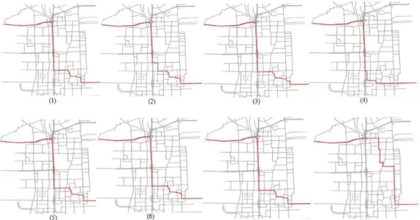
simulation results. Further analysis showed that route choices were biased toward the ring roads, yet the adjustment of the route choice model parameters had little effect in mitigating the bias. It was therefore suspected that an inherent limitation of MNL played an important role there. MNL has a critical limitation in terms of its assumption that the error terms are identically and independently distributed (i.i.d.). Such an assumption generally does not hold in an urban network with overlapping alternative paths. Specifically in the Beijing network, a large number of paths share the same expressway links. See an example in Figure 2-1 for a subset of the choice set for a certain OD pair (the average route choice set size is around 30). As a result, it was likely that the MNL route choice model significantly over-predicted the probabilities of choosing paths containing expressway links, which led to unrealistic congestion along those roads.
Figure 2-1 Overlapping Paths for OD Pair 1616-1584 (Note: The choice set has more than 8 paths.)
To tackle this problem, researchers have followed two major lines of research. One is to abandon the MNL model and consider the correlations among overlapping paths explicitly, e.g., Probit (Daganzo, 1977; Yai et al., 1997), Cross-Nested Logit (Vovsha and Bekhor, 1998), Error
Component (Bekhor et al., 2002; Frejinger and Bierlaire, 2007). The other approach, which is the focus of this paper, adds a deterministic correction term to the MNL utility function for
overlapping paths to take advantage of the simplicity of MNL and the resulting applicability to real-life networks. The first attempt was made by Cascetta et al. (1996). They added a
“commonality factor” (CF) term to the deterministic part of the utility function that captures the degree of similarity between alternatives in the choice set. The modified model is referred to as the C-Logit model, where Pn(i) , the probability of user n choosing path i among his/her
individual choice set Cn, is defined in Equation (2-1):
Pn(i)= e Vin−CFin eVjn−CFjn j∈Cn
∑
. (2-1)Here Vin is the systematic utility of path i for individual n, the deterministic part (before adjustment) of the total utility and CFin the commonality factor. Four different forms for the commonality factor correction were suggested, but no guidance was provided as to which form should be used.
Motivated by the C-Logit model, Ben-Akiva and Ramming (1998) proposed the Path-size Logit Model (PSL) (see also Ben-Akiva and Bierlaire, 2003), which had a similar form but used a “Path Size” (PS) attribute (instead of the CF term) as the correction for the utility for overlapping paths. The PS attribute was originally derived from the discrete choice theory for aggregate alternatives (Ben-Akiva and Lerman, 1985), and was intended to reflect the fact that an
overlapping path was perceived as less than an elementary alterative (with a “size” less than 1), in analogy to an aggregate alternative (e.g., a zone in a destination choice model) perceived as more than one elementary alternative (with a “size” greater than 1). Ben-Akiva and Ramming (1998) defined the correction term PSin as the “size” of the path i, as in Equation (2-2):
PSin = la Li a∈Γi
∑
1 δaj j∈Cn∑
. (2-2) where Γi is the set of links on path i, la the travel time on link a, Li the total travel time on pathi, Cn the choice set of paths for individual n, and δaj a binary variable which equals 1 if link a is a part of path j and 0 otherwise. Note that PS is not affected by link segmentation, as the
contribution of each link is proportional to its travel time to the path travel time. For a path not overlapping with any other path, the path size is 1, and the systematic utility is not adjusted. For a path partially overlapping with other paths, the path size is less than 1, and the systematic utility is downwards adjusted. For a path completely overlapping with J – 1 other paths (J being the size of the choice set Cn), the path size is 1/J. Note that static link travel times are generally used in the calculation, as the PS variable is designed to reflect a traveler’s perception of an alternative’s “size” that should not change in a within-day context (e.g., from 8:00am to 8:15am). Further empirical evidence is desired to validate the hypothesis.
Once the PS attribute is defined, the utility associated with path i for individual n is adjusted as
Vin+ lnPSin, and the path choice probability Pn(i) is computed as in Equation (2-3):
Pn(i)=
eVin+ln PSin
eVjn+ln PSin
j∈Cn
∑
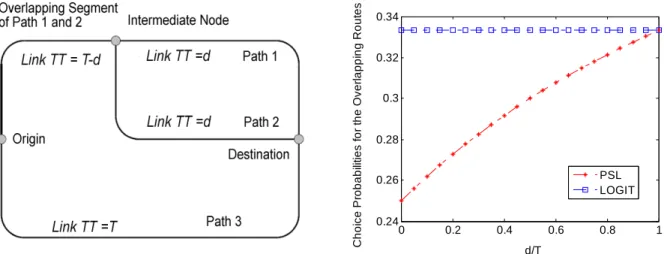
. (2-3) An example as shown in Figure 2-2(a) has been used in the literature (e.g., Cascetta et al. 1996; Ramming, 2002) to illustrate the overlapping path problem. Ramming (2002) has shown how the PSL choice probabilities compare with other model types, especially with MNL model. There are three paths with the same total travel time T. Paths 1 and 2 overlap from Origin to Intermediate Node with an overlapping travel time of T-d. The MNL model will predict equal shares for the three paths, one third each. This is correct only when d=T, i.e., there is no overlap. The choice probability as a function of non-overlapping fraction (d/T) for the overlapping path (Path 1 or 2) is presented in Figure 2-2(b). When the fraction approaches zero, Paths 1 and 2 are the same physical path with two separate "labels". In this case, we expect that the combined choice probabilities for Paths 1 and 2 are 50%, and Path 3, the other physical path, should have a choice probability of 50%. The PSL reflects our expectation, but the MNL model gives a flat choice probability at 33% that is not sensitive to the overlapping.0 0.2 0.4 0.6 0.8 1 0.24 0.26 0.28 0.3 0.32 0.34 d/T C h oi c e Pr ob ab ili ti e s f o r th e O v er la pp in g R o ut es PSL LOGIT
Figure 2-2 (a)The Overlapping Path Problem; (b) Choice Probabilities for the Overlapping Path Network
Consider a similar example in the context of complicated urban networks, where a traveler
makes route choice from home to work. The overlapping segments usually lie on the expressway, and there are N different paths to the work place after getting off the expressway. In addition, he/she has another alternative to use the arterial road right after leaving home. Suppose, in the simplest case, all the N + 1 paths have the same travel time. If the overlapping segment is sufficiently long, we can expect the probability of the freeway being chosen is approximately 50%, which is in accordance with the prediction given by the PSL model. However, the MNL model will give a probability of N
N+1 to the expressway, and a probability of 1
N+1 to the arterial. This indicates more demand will be allocated to the expressway when N is greater than one. In a dense urban network, N is potentially very large, and therefore the bias could cause serious congestion in the traffic simulation model.
Recognizing such an issue with MNL, we verified that this bias existed in the simulation of the Beijing network (Wei, 2010), and adopted PSL for modeling route choice. After the
enhancement, the gridlock situation was mostly resolved, and the route choice led to a more realistic traffic flow and density distributions on the network.
2.2 Lane Groups
In the supply models used by DTA systems, roads are typically modeled as links connected at intersections (modeled as nodes). In some models, it may also be possible to divide a link into multiple segments to capture within-link capacity changes due to, for example, changing section geometries such as the number of lanes. Each segment may contain two parts with distinct traffic behaviors: a “moving part” starting from the upstream side of the segment where vehicles
entering the segment can move at a relatively high speed and a dynamic “queuing part” at the downstream end of segment where stop-and-go traffic is present. The boundary of the moving
part and the queuing part depends on the traffic condition on the segment and may vary as the simulation proceeds. In the moving part, in-flow vehicles typically move at a certain speed governed by the speed-density relationship, while in the queuing part, (lane- or link-based) queues are formed following a queuing model. The ability to explicitly model queuing in its supply model is a crucial feature for DTA systems to realistically estimate congestion.
Without loss of generality, we assume the within-link supply model is defined at a segment level, i.e., each segment has its own set of supply parameters describing the speed-density relationship and the capacities. For those models that only have links defined but no explicit segment
representations, they can be thought of as a one-segment-per-link special case.
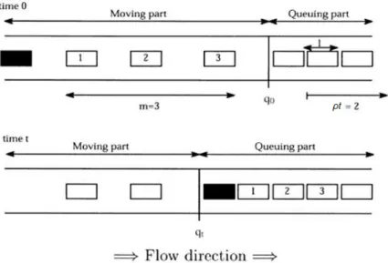
One of the simplest queuing models used by DTA is a deterministic queuing model illustrated in Figure 2-3 (see, e.g., Ben-Akiva et al., 2001 and the references therein). During a time period of length t (usually the simulation time step in the range of one to several seconds) starting at time 0,
ρt vehicles leave the queue, where ρ is the output capacity of the segment. At time t, given that
there is a vehicle reaching the end of the queue, the position of the end of the queue is calculated as: ) ( ) 0 ( ) (t q l m t q = + −ρ , ··· (2-4) where q(0) is the position of the end of the queue at time t = 0, l the average length of vehicles (including headways), and m the number of moving vehicles between the vehicle in question (in black in Figure 2-3) and the end of the queue at time t = 0. Here the position of the queue is measured from the downstream end of the segment.
Note that the model is relevant only when 0 ≤ q(t) ≤ L, where L is the length of the segment. If
q(t) < 0, it means that the queue has already dissipated by time t and q(t) should be set to 0. As
the segment storage capacity is explicitly accounted for when vehicles from upstream segments are entering, the number of vehicles on the current segment will never exceed its storage capacity and thus q(t) > L will never occur.
Figure 2-3 Deterministic Queuing Model
Different DTA models may treat the queue in different ways. Some models build a single queue for each segment, while others allow separate queues to form on individual lanes and vehicles in one lane does not block movements in others. Most existing mesoscopic simulation studies employ segment-level implementations of queues, ignoring the lane connection restrictions at the intersections. In other words, if two segments are connected at the intersection, all lanes on the upstream segment are connected to all lanes in the downstream segment. This is probably because networks and lane restrictions for many previous studies are not complicated enough (e.g., highway networks) to entail the non-trivial efforts required for the implementation of explicit lanes, such as coding lane connection restrictions and dynamically switch between a lane-based and segment-based representation according to the queue length. The segment-level queuing model also has the run-time efficiency compared to the more elaborate lane-based one. Segment-based queuing models are simple to implement yet they have drawbacks. One of them is the blocking effects between different movements. Specifically, queues spilled back from the downstream segment can be mistakenly allowed to form in all lanes in the upstream segment. For instance, the left turn queue may block the through and right turn traffic because the model will generate a single queue for the segment, regardless of the turning movement (Figure 2-4). In our study network of Beijing, lane restrictions at complicated intersections are commonly seen. Moreover, on- and off-ramps connecting the expressways and side roads are often highly
congested. Consequently, lane restrictions have significant impact on the throughput of those intersections. Unrealistic congestion caused by an exit queue blocking through traffic was found to be one of the major reasons of gridlock at the early stage of our study, as we initially used the segment-based queuing model in DynaMIT.
Liu et al. (2008) proposed a set of lane group-based macroscopic formulations to address such drawbacks. Chiu & Villalobos (2008) also presented the lane group structure in AMS, a
mesoscopic simulator. This structure is designed to account for spillbacks from downstream segments and ensure that vehicles located in turning bays do not artificially impede through traffic. DynaMIT was initially designed with capability in flexible network representation (Ben-Akiva et al., 2001). Its model allows both segment-based queuing as well as lane-based queuing, in which case the lanes serving the same direction can be put into lane groups.
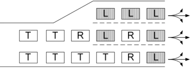
Figure 2-4 Left-turn lane block the through and right turn traffic
To address the aforementioned issue, a lane-based queuing model should be used and in our study “lane groups” are used to capture the lane restrictions. A lane group is defined as a set of lanes established at an intersection approach for separate capacity and level-of-service analysis (Transportation Research Board, 2000). In a lane group model, lanes are grouped according to their specific turning movements. For example, Figure 2-5 shows an approach to an intersection with the queuing part comprising of three lane groups: left only, through, and right only. Note that in a mesoscopic model lane groups are only relevant for the queuing part of the segment; there is no need to distinguish which lane a vehicle is on when it is in the moving part (i.e., there is only one lane group that contains all the lanes). This reduces the complexity of the moving part and helps improve the run-time efficiency.
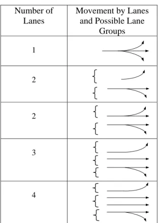
To effectively apply the lane group-based queuing feature, the construction of lane groups should take into account both geometry changes and lane restrictions at intersections. We generated the lane connections following the guideline given by Highway Capacity Manual (Transportation Research Board, 2000). Table 2-1 shows the typical lane groups for analysis.
Table 2-1 Typical Lane Groups for Analysis
Number of Lanes
Movement by Lanes and Possible Lane
Groups 1 2 2 3 4
Constructing the lane group information in the model required non-trivial work, especially if the lane restrictions information were initially missing as it was in our case. In addition to the manual work to verify lane restrictions at the intersections, extra care was paid to calibrate the capacities for the lane groups. The effort proved to be necessary in our Beijing network -- with a queuing part based on lane groups, the mistakenly formed queues due to the limited capacity from another lane group were removed, and a large number of unrealistic bottlenecks
disappeared. This feature combined with the Path-size Logit model contributed significantly in resolving the unrealistic gridlocks generated in the simulations.
2.3 Short links
Short links are not uncommon in real-world networks. The Beijing network, for example, has complicated interchanges (such as the one shown in Figure 2-6) with many short links, some of which are around the length of a car. Such links are often seen at an at-grade intersection
connecting two same-direction roadways separated only by a divider. For models whose network representation maintains high fidelity to the real-world road network, short links are kept as the
way they are, rather than removed to obtain simplified intersections. This in turn poses challenges for the model to replicate realistic traffic dynamics.
Figure 2-6 A complicated interchange with short links
During the early stages of our simulation study in the Beijing network, we observed excessive congestion originated from those short links. It turned out that the congestion resulted from two distinct types of problems: 1) vehicles moving unrealistically slowly on short links, and 2) vehicles queuing unnecessarily upstream of a short link. As the causes of the two problems are different, they are discussed separately in the rest of this section. The commonality between the two problems is that inaccuracies introduced by approximations in a mesoscopic supply model for it to run efficiently in a congested real-world network are magnified to an extreme extent on very short links.
Following the modeling terminologies introduced in Section 2.2, the discussion will be based on segments for the moving part problem in Section 2.3.1 as no lane group details are needed for the moving part, and based on lane groups for the queuing part problem in Section 2.3.2.
2.3.1 The unusual impact of the minimum speed on short segments
An abnormal phenomenon we observed was that vehicles moving at a normal/high speed on the relatively long segments might decelerate to an unnecessarily slow speed on the short segments. When investigating the cause of the problem, we realized that, for shorts segments, the length of a segment might play a significant role in the calculation of the speed of a moving vehicle, which is otherwise negligible in a network with relatively long segments.
In the mesoscopic traffic simulators of many DTA models, the speed of a vehicle at the moving part of a segment is governed by the segment’s speed-density relationship, which might take a form similar to the one in Equation (2-5) :
⎪⎭ ⎪ ⎬ ⎫ ⎪⎩ ⎪ ⎨ ⎧ ⎟ ⎟ ⎠ ⎞ ⎜ ⎜ ⎝ ⎛ ⎟ ⎟ ⎠ ⎞ ⎜ ⎜ ⎝ ⎛ − − − = α β min jam min max min ) 0 , max( 1 , max k k k k v v v (2-5)
where v is the speed, k the density, vmin the minimum speed on a segment, vmax the maximum
speed on a segment, kmin the density below which the speed is fixed at vmax and kjam the jam
density. Typically, vmin, vmax, kmin, kjam, α, and β are parameters to be calibrated.
As the speed-density relationship is originally developed for relatively long road segments with stable flows, its application to extremely short segments should be examined carefully. For a short segment, the density increases drastically from zero whenever a car enters the segment. For example, if the segment’s length equals to that of a typical car, then k could only be either 0 or
kjam, which results in two possible calculated speed following Equation (2-5):
⎩ ⎨ ⎧ = = = jam min max if , 0 if , k k v k v v (2-6)
In other words, the speed on this segment will drop to vmin whenever it is occupied, effectively
making the average simulated speed equal to vmin. Hence if vmin is lower than the average
observed speed, this segment would almost always cause unrealistic congestion.
Since the minimum speed vmin is to be calibrated, one possible solution is to increase the starting
value of the calibration variable to the average observed speed for each of those short segments, and restrict this value from deviating too far from the mean. This method was effective for the Beijing study.
2.3.2 The acceptance capacity at the absence of queuing
In mesoscopic traffic simulators, vehicle-to-vehicle interactions at the intersections are often modeled by simple constructs defined at an aggregate level. Specifically, the impacts of traffic signals are often implemented as “output capacities”. A lane group’s output capacity defines the maximum number of vehicles that can move out of the lane group at a given unit of time. Similarly, the rate at which vehicles can enter a lane group is sometimes referred to as the “acceptance capacity”. While output capacities are to be calibrated, the acceptance capacities are dynamically determined by the available space on the downstream lane groups and how fast the vehicles are moving out of these lane groups.
Capacities control various aspects (such as the spillbacks) of the queuing behavior in the
mesoscopic simulation models. A queue for a given turning movement is formed on a lane group when either the output capacity of the lane group or the acceptance capacity of the downstream lane group is binding. In other words, the “effective capacity” – the actual flow rate leaving lane group j at time t – can be computed as in Equation (2-7):
Ceff jt = min(C out jt , Cacc′ j t ) ··· (2-7)
where Coutjt is the output capacity of lane group j at time t, and Caccj t′ the acceptance capacity of lane group j’, the downstream lane group of lane group j, at time t. Note that for discrete time-based simulation models, “time t” actually means “time-step t”.
Caccj t′
is determined by the available space the downstream lane group j’ has. The more vehicles are on the downstream lane group, the less acceptance capacity it has. For time-based simulation models, the acceptance capacity at time t is often computed from the lane group’s available space at time (t- 1), as shown in Equation (2-8):
Cacc ′ j t =L ′ j • mj ′ / L − (nj (t′ −1)−Δnj t′ ) ΔT ··· (2-8)
where Lj ′ is the effective length of lane group j’, mj ′ the number of lanes in lane group j’, L the average effective vehicle length, nj (t′ −1) the number of vehicles on lane group j’ at time (t-1),
Δnj t′
the (expected) number of vehicles to move out of lane group j’ between time t-1 and t, and
T
Δ the time-step size.
Note that the number of vehicles moving out of lane group j’ depends on the speed and capacity of the current lane group and its downstream lane group. Therefore, at the beginning of time-step
t, Δnj t′
is generally unknown, unless the current and downstream lane groups have been
processed in the simulation. Typically, the simulator may need to “guess” the value of Δnj t′ . For example, one could use the value from the previous time-step (Δnj t′ −1), or even simply assume a value of zero.
When the assumed Δnj t′ is smaller than the actual value, the acceptance capacity is effectively underestimated. However, one may argue that the impact of Δnj t′ is not as significant as it appears. Roughly speaking, if the network is not too congested and lane group j’ has sufficient space, then the binding constraint in Equation (2-7) is likely to be Cout
jt
(as long as Cout jt ≤ C
acc
′
j t
). On the other hand, if the network is congested and lane group j’ does not have much available space, then Δnj t′ is likely to be small, as vehicles tend to move slowly and the downstream lane
group j’ may have queues preventing a fast discharge. Therefore, under most circumstances, the underestimation caused by Δnj t′ is insignificant.
While the above argument may hold when the lane group is sufficiently long, it is not the case for short links (and thus short lane groups). Suppose the downstream lane group j’ can only hold one vehicle, i.e., Lj ′ = L , and mj ′ =1. If we ignore Δnj t′ , then whenever there is a vehicle on it (i.e., nj (t′ −1)=1), its acceptance capacity computed from Equation (2-8) is zero, in which case “no more space is available on the lane group”. In reality, however, if the vehicle is moving, as soon as it moves out the lane group, another vehicle can be accepted.
Failing to recognize the inaccuracy in the calculation of acceptance capacities may over-predict congestion, especially for highly congested networks or real-time applications. In those
situations, for computational efficiency considerations, typically the acceptance capacity is not updated every time a vehicle is moved; instead, it may be assumed constant for a short period of time (such as a minute). In such cases, if there is a vehicle on the short lane group when the acceptance capacity is updated, the acceptance capacity stays zero during the whole period until the next update, and this effectively blocks the upstream traffic unnecessarily.
Our solution is to ignore the acceptance capacity constraint when there is no queue in the downstream segment (and thus the lane group is the segment), namely using Equation (2-9) instead of Equation (2-7): ) , min( accjt t j q jt out jt eff C M C C = δ ′ + ′ ··· (2-9) where δq ′ j t
is a binary variable which equals 1 if there is no queue on lane group j’ at time-step t and 0 otherwise, and M an sufficiently large positive number (a practical positive infinity). Equation (2-9) is equivalent to Equation (2-7) when there is a queue on lane group j’; however, when there is no queue, δq
′
j tM+ C acc
′
j t
is always greater than Coutjt, making the output capacity binding and thus ignoring the acceptance capacity.
After accounting for the vehicles’ moving state, a revised capacity model was implemented in the DTA model, and the abnormal queuing phenomenon was eliminated.
2.4 Variable output capacity
In urban networks (as often seen in developing countries), the mixed traffic condition is commonly seen. The impact of bicycles and pedestrians on road intersections, for example, cannot be ignored. To model this impact, we introduced the variable output capacity in the DTA model. Note that we only dealt with the impacts of non-motorized traffic on vehicular traffic, but not those of vehicular on non-motorized traffic. A more comprehensive treatment of the issue should include the two-way interaction between them.
As briefly described in Section 2.3.2, the output capacity is a parameter for each lane group (or segment) in the supply model, and it is typically calibrated and validated offline. In most previous studies, the output capacity was fixed during the whole simulation period, i.e., Cout
jt
in Equation (2-7) or Equation (2-9) was constant across all possible time-step t. We refer to it as static capacity.
Static capacity does not fully reflect the traffic situation with significant interferences from bicycles and pedestrians, which may cause capacity reductions for motorized traffic at the intersections, especially during rush hours. Since most bicycle and pedestrian trips are for commuting purposes, their flows are also time-dependent. Therefore, the conflicts between bicycles/pedestrians and vehicles are different during different times of the day. To capture such time-dependent capacity reductions, we should drop the static assumption on Coutjt and make it a time-dependent variable.
In our model with dynamic output capacity, for each lane group, the output capacity may assume different values at different time-of-day; those values are treated as parameters to the supply model, and can be calibrated during the off-line calibration process. This small relaxation brings the flexibility of variable output capacity to our model, and avoids the unnecessary constraints that would potentially reduce the fit of the calibration.
3 Case Study
3.1 DynaMIT-P
In this case study, we used the DynaMIT-P (Dynamic network assignment for the Management of Information to Travelers) DTA system to model a highly congested urban network in Beijing. DynaMIT-P is a simulation-based DTA system (Ben-Akiva et al. 1997, 2001, 2002) for planning applications. It uses a built-in microscopic demand simulator, which disaggregates the OD flows and simulates individual vehicles’ choices, a mesoscopic supply simulator, which simulates the moving of vehicles whose speeds are governed by macroscopic speed-density relationships instead of micro-level vehicle-to-vehicle interactions, and captures complex demand-supply interactions. It models travelers’ short-term and within-day decisions, such as choices related to trip frequency, destination, departure time, mode, and routes, assuming the long-term travel decisions (such as residential locations and auto-ownership) are given. Details about the features and framework of DynaMIT-P can be found in Appendix A of Balakrishna (2006). The travel decisions are modeled in the discrete choice framework (Ben-Akiva and Lerman, 1985), where the aggregate OD flows are converted into individual vehicles (packets) through DynaMIT-P’s demand simulator. The route choice set for each OD pair is generated in the pre-processing stage using a combination of the link elimination and simulation methods (Chapter 3.2, Ramming, 2002). The packets with the chosen routes are then simulated in the mesoscopic supply simulator to obtain the network performance measurements such as time-dependent flows, travel times,
to significantly shorten the running time for the simulation of the network in comparison to typical microscopic traffic simulators.
In previous studies, DynaMIT-P and its corresponding real-time version have been applied successfully in major cities in the United States. In Los Angeles, California, a real-time version was calibrated and deployed as a route guidance system in the South Park area for traffic state estimation and prediction (Wen et al., 2006a, 2006b). In Lower Westchester County, New York, DynaMIT-P was combined with NYSDOT’s ITS infrastructure for traffic condition
improvements (Rathi et al., 2008). In Boston, Massachusetts, DynaMIT-P was used for the evaluation of emergency evacuation plans (Balakrishna et al., 2008). The Beijing study is, however, the first highly congested urban network DynaMIT-P is applied to.
3.2 Network and Data
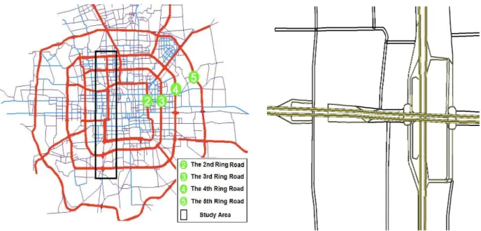
Beijing, China is one of the ten most populated megacities in the world. In recent years, the vehicle volume has increased at an annual rate of 20 percent. In 2008, there were reportedly 3.5 million registered motor vehicles (the number reached 4 million at the end of 2009), of which 2.3 million were private passenger cars. Urban trips within the Sixth Ring Road, the outermost ring road of the city, reached 35 million trips per day (including 8.8 million walking trips). The significant pressure on the transportation system results in severe traffic congestion and air pollution. As an illustration of the traffic problem, Figure 3-1 shows the link volume-over-capacity (V/C) ratios during morning peak hours on weekdays in 2007 from a static
transportation planning package, where red roughly indicates a level of service D (Transportation Research Board, 2000) or worse.
As shown in Figure 3-2, the skeleton of Beijing urban transportation network comprises a series of ring roads connected by arterial roads, and the area for our study is the West 2nd Ring Road network and its northern and southern extensions. Several major ring roads and arterial roads intersect the 2nd Ring Road within this area resulting in 14 interchanges. The ring roads are elevated roadways supplemented by parallel side roads with frequent on- and off-ramps. These ramps are generally spaced between 200 to 600 feet to ensure access to and egress from the ring roads (Figure 3-3). The network under study passes the center of the city and it is not
uncommon for the northern part of the West 2nd Ring Road to be in a complete jam condition extending several miles. The situation is further complicated by the presence of unusually short links – some as short as 20 feet, which could cause unexpected problems for the simulation model. Modeling such conditions is difficult because the congestion is so severe that a small over-estimation in the demand or a small under-estimation in the supply capacity would result in a gridlock.
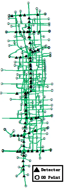
The computer representation of the study network consists of 1,698 nodes connected by 3,180 directed links (Figure 3-4) in an area of around 18 square miles. The historical dataset includes static demand during the AM peak hours for 2,927 non-zero OD pairs, derived from the most recent household surveys and calibrated against counts and speeds from Remote Traffic
Microwave Sensors (RTMS) and travel times from Floating Car Data (FCD). The static demand was processed to derive an initial time-dependent demand in 15 minutes intervals. The
simulation ran from 6:00am to 10:00am. The demand was assumed fixed and approximately 630,000 vehicles were simulated.
3.2.1 Surveillance Data
Surveillance information used in the Beijing case study includes traffic counts and link travel times from six weekdays during December 2007 between the hours of 6:00am and 10:00am. The traffic counts were obtained from RTMS. Within the study area, there were altogether 154 RTMS detectors deployed. Most of them (the triangles shown in the Figure 3-4) were on the expressways. It was reported that 140 of those sensors were functioning normally, providing 24-hours traffic flow information continuously.
The link travel times are extracted from the FCD, which was obtained from GPS (Global
Positioning System) equipped taxi fleets. Nearly 90% of all the major roads in Beijing, including expressways, ramps, arterials, secondary roads and local roads, are covered by the FCD, which can partially make up for the lack of count observations on arterials and local roads.
Both count and travel time data were processed by Beijing Transportation Research Center (BTRC); we did not have access to the raw data. Particularly, the observed counts were
aggregated in 1minute intervals, while the link travel time data were provided as averages at 5-minute internals. Additionally, some initial pre-processing was done to remove observations from malfunctioning sensors. Over the four-hour study period, we eventually received 1,694 traffic count observations, and 52,545 link travel time observations.
Figure 3-4 Network of the study area
3.3 Calibration
3.3.1 Calibration variables
the Beijing network before we can use it for further applications and analysis. Specifically, a total number of 69,093 variables were identified, and these include
• 46,832 time-dependent OD flows from 2,927 OD pairs over the 16 time periods, each of which corresponds to a 15-minute interval from 6 AM to 10 AM.
• one coefficient of travel time βTT in the route choice model to compute the path utility
Vi=βTTTTi, where Viis the systematic utility of path i and TTiis the travel time on path i. In
an ongoing study, a more elaborate route choice model is estimated with individual GPS traces and then incorporated into the DTA model. The results will be reported in a succeeding paper.
• 19,080 speed-density parameters (6 parameters, vmax, kmin, kjam, α, β and vmin for each
segment); and 3,180 segment capacities of ring roads and arterials. Lane group capacities are not calibrated separately, and calculated as fractions of the segment capacities based on the number of lanes in the lane group. Note that given the study period is during the AM peak when the bicycle and pedestrian interferences are constantly high, the segment capacities are treated as static, although the time-dependent capacity feature is implemented in DynaMIT-P.
3.3.2 Methodologies for calibration
All the demand and supply parameters of DynaMIT-P are calibrated simultaneously. The calibration problem is formulated as a constrained minimization problem. Let the time period of interest be divided into intervals h = 1,2,...,H. Let xh denote the vector of OD flows departing from their respective origins during time interval h. Let
β
h be the vector of simulation model parameters that must be calibrated together with the OD flows. The objective function is a weighted sum of distances between time-dependent location-specific simulated measurements and field measurements (both counts and link travel times) and distances between calibrated variable values and their respective a priori values.∑
= ⎥⎦ ⎤ ⎢⎣ ⎡ − + − + − + − H h a h h a h h t h t h c h c h x x H H 1 w B F w B F w x x w 2 4 2 3 2 2 2 1 ,..., , ,... 1 1 minimize β β β β (3-1)subject to the following constraints:
{
H}
h g g g u l u x l G G x x f F F h n h h h h h x h h x h h h h t h c h ,... 2 , 1 , 0 ) ( , , 0 ) ( , 0 ) ( ) ,..., , ..., , ..., ( ) , ( 2 1 1 , 1 , 1 ∈ ∀ ⎪ ⎪ ⎭ ⎪ ⎪ ⎬ ⎫ = = = ≤ ≤ ≤ ≤ =β
β
β
β
β
β
β β K , (3-2)where Bh c
and Fh c
are the observed and fitted counts for interval h respectively, Bh t
and Fh t
the observed and fitted link travel times for interval h respectively, xh
a
and βh a
the a priori values of OD flow xh and model parameters βh for interval h respectively. f( ), the simulation-based
DTA model, takes as arguments the OD flows xh, the network Gh and model parameters
β
h up tointerval h. lhx and uhx are the lower and upper bound of OD flow xh, and lh
β
and uhβ the lower and upper bound of model parameters
β
h. gi( ) is a function that specifies the physical relationshipbetween the model parameters, e.g., the free flow speed, vmax cannot be smaller than the
minimum speed, vmin, and n is the number of such physical relationship expressions. The weights
w1, …, w4 depend on the relative confidence one can attribute to the corresponding
measurements and a priori values. For example, if sensors are not reliable, a lower weight might be put on counts. The weights also depend on the order of magnitude of the measurement in order to avoid a situation where a parameter with a bigger magnitude or more observations dominates the others in the fitting function.
Initially, we attribute a weight of 1 (w1) to the sensor count measurements, 0.05 (w2) to the
floating car travel times due to the high volume of observations, and 1 (w3) to the a priori values.
These weights are adjusted dynamically during the calibration in response to the performance of the SPSA iterations to accelerate the optimization process.
Note that to avoid the potential problem of over-fitting with the large number of calibration variables, the distances from the a priori values of the OD flows and model parameters are included in the objective function, where the a prior values are the best results achieved through manual adjustment whose reasonableness has been checked. The bounds on the parameters and their physical relationships in Equation (3-2) also ensure that the variables will not take
unrealistic values.
The optimization problem is solved using the Simultaneous Perturbation Stochastic
Approximation (SPSA) algorithm, originally developed in Spall (1992, 1998, and 1999) and applied to DTA calibration in Balakrishna (2006) and Balakrishna et al. (2006). The SPSA algorithm is attractive for large problems because of its efficient gradient approximation by perturbing all variables at once. It is also designed for stochastic problems and allows for inputs corrupted by noise, which is usually the case in simulation-based DTA models.
In each SPSA iteration, DynaMIT-P is run three times. Two runs are needed to generate the gradient approximation, and a third run to produce traffic conditions with the adjusted
parameters. Output link travel times from this run are then used as input link travel times to the demand simulator of DynaMIT-P for the next SPSA iteration. The difference between the input and output link travel times measures the convergence of the fixed-point problem of demand-supply interaction and is monitored over iterations. On a computer with an Intel Core 2 Duo processor at 2.00GHz, each DynaMIT-P run takes around 8 minutes and uses around 1GB
3.3.3 Results
The quantification of errors in the model performance is important for the evaluation of the calibration. The fit of counts and travel times are computed across all reliable sensors and all available floating car observations. The following two error statistics have been adopted to measure the discrepancies between observed (yi) and simulated ( ?y i) quantities, where S is the
dimension of the unknown vector:
• Root mean square error (RMSE) (Pindyck and Rubinfeld, 1997)
RMSE= (yi− ?y i) 2 i=1 S
∑
S (3-3)• Normalized root mean square error (RMSN) (Ashok and Ben-Akiva, 2002)
RMSN= RMSE yi i=1 S
∑
⎛ ⎝ ⎜ ⎞ ⎠ ⎟ /S (3-4)The first 30 minutes of the study period (6:00am-10:00am) is used to warm up and load the network. Thus the calibration and evaluation is limited to 6:30am to 10:00am.
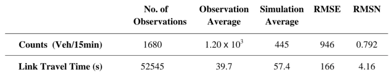
A lower value of RMSE or RMSN indicates a lower discrepancy between the simulation results and the observations. The calibration starting point in terms of error statistics is given in Table 3-1:
Table 3-1 Model fit before the calibration
No. of Observations Observation Average Simulation Average RMSE RMSN Counts (Veh/15min) 1680 1.20 x 10³ 445 946 0.792
Link Travel Time (s) 52545 39.7 57.4 166 4.16
The parameters for the SPSA algorithm and objective function weights are adjusted during the calibration to accelerate the process. The objective function value usually changes significantly right after an adjustment. Figure 3-5 shows the last 530 iterations of SPSA, where the weights and SPSA parameters are kept constant. The objective function value does not always decrease over iterations, since the problem is stochastic and the gradients are approximated. The
improvement in the objective function value at the end of calibration indicates that the SPSA algorithm is appropriate for this particular problem (note that it is not guaranteed the global minimum has been found). The RMSN between the time-dependent input and output link travel
times from these iterations is stable and about 0.08, which suggests that an equilibrium state has been reached.
The calibrated model reflects the high congestion level in the study area. Over the course of the simulation, queues appear on 591 links, among which there are 33 spillbacks (one spillback is a set of concatenated links where the queue on the most downstream link spillbacks to all upstream links). The longest spillback extends 3.20 kilometers (1.99 miles) and the average length of spillback is 441 meters (0.274 miles).
Figure 3-5 The trend of objective value for the last 530 iterations Table 3-2 Overall calibration results
No. of Observations Observation Average Simulation Average RMSE RMSN Counts (Veh/15min) 1680 1.24 x 10³ 1.23 x 10³ 384 0.308 Link Travel Time (s) 52545 39. 7 38.7 17.3 0.436
Table 3-2 contains the error statistics on the fit to counts and fit to link travel time across all time horizons.
Figure 3-6 Calibration results for the peak periods (left: 8:30-8:45; right: 8:45-9:00)
An intuitive illustration is given in Figure 3-6 for the fit-to-counts during the peak periods from 8:30 to 9:00AM. The x-axis is the observed sensor counts and the y-axis is the calibrated sensor counts. The 45-degree line indicates a perfect match between the simulated counts and the observed counts. The sensors with counts deviating more than 50% from the observed values were marked with sensor numbers. Most of the observed and simulated sensor counts fall around the 45 degree line, indicating that most of the deviations between the simulated and observed counts are within an acceptable range.
Figure 3-7shows the RMSN and RMSE of counts at different flow rates. The first group gives the overall calibration result, and the remaining ones are by flow rate levels: high
(>1400veh/15min), medium (1000-1400 veh/15min), low (0-1000 veh/15min). Each group contains three bars, indicating the data average, simulation average and RMSE respectively. The RMSN for each group is noted above the bars. The small difference between the data and simulation averages suggest that the calibration is unbiased. It is also found that the high and medium groups have better fits than the low-flow group. The best fit to count exists in the high-flow group with a RMSN around 25%.
A previous DynaMIT application in Los Angeles, CA (Wen et al., 2006a, 2006b) had RMSN for counts in the range of 20% to 24% depending on the road type. The Beijing case study has a more complicated network, higher demand, more calibration variables, and smaller number of count stations, and it is not surprising that the model fit cannot achieve the previous levels. Similar analysis on floating car travel time was conducted and is shown in Figure 3-8. The floating car data are grouped into four categories according to link travel time: 0-20 seconds, 20-40 seconds, 20-40-60 seconds and longer than 60 seconds. The best fit for travel time is reached in the range of 40-60 seconds, with a 26% RMSN.
In-depth analysis was also performed on the path travel time in order to better evaluate the model capability of replicating realistic traffic situation. Since the floating car data are given in the form of link by link travel time, not every link in an OD path has floating car data available. In order to carry out this analysis, given a set of paths for an OD pair, we have to check the data
availability in the floating car data first. In our case, we found 3996 paths with floating car data available. The comparisons between simulated and observed path travel time is given in Figure 3-9. Most of the red dots are around the 45 degree line, indicating a good match of the simulated path travel time with the observed data.
Given the large number of calibration parameters, it is likely that there are multiple local minima to the optimization problem. The SPSA algorithm is generally notable for its ability to find the global minimum for problems corrupted by noises (Spall, 1992; Spall, 1998; Balakrishna, 2006), yet we still checked the reasonableness of the calibrated parameters manually with engineering judgment to gain more confidence on the results.
Figure 3-7 Fit to counts
Overall 0-1000 1000-1400 >1400 0 200 400 600 800 1000 1200 1400 1600 1800 2000 Cou n ts (v eh / 15 min u te s ) Sample Size:1680 Sample Size:459 Sample Size:657 Sample Size:564 RMSN=0.30 RMSN=0.45 RMSN=0.31 RMSN=0.25 Data Average Simulation Average RMSE
Figure 3-8 Fit to link travel times 0 100 200 300 400 500 600 700 0 100 200 300 400 500 600 700
Observed Path Travel Time
S im u lat ed P a th T ra v el T im e Observed average = 65.17s Simulation average = 63.20s RMSE = 13.16 RMSN = 0.20
Figure 3-9 Fit to path travel time analysis
Overall 0-20 20-40 40-60 >60 0 20 40 60 80 100 120
Group by link travel time (seconds)
L ink T ra v e l T ime( s e c onds) Sample Size: 52545 Sample Size: 21165 Sample Size: 12945 Sample Size: 7410 Sample Size: 11021 RMSN=0.436 RMSN=0.492 RMSN=0.305 RMSN=0.268 RMSN=0.329 Data Average Simulation Average RMSE
3.4 Application Analysis
DTA systems like DynaMIT-P, once calibrated, can be used to evaluate various types of traffic management strategies and scenarios. We demonstrate this by conducting an analysis for the short-term benefit evaluation of the “Rotating No-Driving Day restriction” scenario in Beijing. This restriction is a strategy proposed by the Beijing municipal government to reduce pollution and relieve traffic. Implemented as part of a six-month trial that took effect after the 2008 Olympics, it prevents private cars from being on the roads one weekday per week according to a rotation schedule based on license plate numbers. For example, cars with a license plate number ending with 1 or 6 are not allowed to be driven on Mondays. Those with plate numbers ending in 2 or 7 are banned from road on Tuesdays, and so on. This restriction has reduced Beijing’s 3.5 million car network demand significantly.
The initial demand for the base case is estimated from the field observations in the calibration process described in Section 3.3. To model the above mentioned scenario, we decrease the initial demand by 20%, assuming that the last digit of the license plate number is randomly distributed. Note that this is only appropriate for short-term analyses, as it does not account for the long-term demand increase caused by reaction to this restriction strategy if it became a long-term policy. We then compare the simulation results of different scenarios with a control case that does not have the restriction. First, we focus on the two most congested areas of interest for transportation management. The GuangAnMen area (Figure 3-10) and XiZhiMen area (Figure 3-11) are two areas that typically experience bottlenecks on the West 2nd Ring Road during the AM/PM peak hours. The pictures below are screenshots of the simulation results during the same time period, for different scenarios, in each location. The pictures on the left correspond to the results of the Rotating No-Driving Day restriction. The pictures on the right present the control case without any restriction (base-case). As shown in the legend, the color of the segment denotes its density, with red indicating high density and thus severe congestion. It is found that the reduction of demand resulted in significant drops in link densities.
Quantitative analyses have also been performed, and several criteria are considered as summarized in Table 3-3:
(1) Number of vehicles reaching the destinations. In the scenario with restrictions, the number of vehicles that reach their destination during the simulation time period (i.e., 550,588, as shown in Table 3-3) is only 8.4% less than the control (base) case, although the overall traffic demand is 20% less. This implies that the Rotating No-driving Day restriction improved the network throughput significantly.
Figure 3-10 GuangAnMen Area, 7:00AM, Restricted Case (left) vs. Base Case (right)
Figure 3-11 XiZhiMen Area, 7:15AM, Restricted Case (left) vs. Base Case (right)
(2) Average travel time. Under the restriction scenario, the overall average travel time, aggregated from the travel time of every vehicle that reaches its destination within the simulation time period, is about 2 minutes less (or 17.9%) than the control scenario. The average travel time for some major OD pairs is also calculated individually, and
consistent reduction is observed. For example, the average travel time from the south end to the north end of the study area is about 45 minutes, which is 20% less than the base case.
(3) The number of links with long queuing time. The queuing time of a link is defined as the amount of time during which the link has one or more lanes containing queues. The
number of links with queuing time longer than 30 minutes is reduced by 50% under the restriction scenario.
Overall, based on the simulation results, imposing such a restriction policy on demand could significantly increase road efficiency and reduce congestion in the short term. This case study demonstrates the enhanced DTA model’s ability to evaluate traffic management strategies.
Table 3-3 Analysis of Rotating No-Driving Day Restriction
With Restriction No Restriction Number of vehicles reaching destinations (veh) 5.51 x 10⁵ 6.02 x 10⁵ Average travel time for all OD pairs in the case
study network (seconds)
497 606
Average Travel Time for OD pairs from South end to North end (seconds)
2.70 x 10³ 3.39 x 10³
Number of links with queuing time > 30 min 58 112
4 Conclusion and Future Directions
In this study, we identified important features required for the accurate replication of traffic conditions in highly congested urban networks. Such networks are characterized by large number of short links, complicated intersections and interchanges, frequent on- and off-ramps and
significant interferences from non-motorized traffic. These features include 1) a route choice model which can account for overlapping routes, 2) explicit representations of lane groups to properly model traffic queues and spillbacks, 3) the ability to handle short links, and 4) the impacts of bicycles and pedestrians on auto traffic modeled by calibrated dynamic road segment capacities.
These features were implemented in DynaMIT-P and applied to a highly congested area in Beijing. We calibrated the model using surveillance data including traffic counts from traffic sensors and travel times from floating car data. An application case study demonstrated the ability of the enhanced DTA model to evaluate management strategies for transportation planning.
To further improve our model, we plan to develop and calibrate a new route choice model for Beijing using vehicle trajectory data. In addition, higher quality input including enhanced
network coding and more accurate surveillance data are expected to improve the model accuracy.
Acknowledgements
The authors would like to acknowledge the Beijing Transportation Research Center for providing data and financial support. The authors are also grateful for Lu Lu’s contribution in running some of the simulations.
Bibliography
Aerde, M. V., Hellinga, B., Baker, M., & Rakha, H. (1996). INTEGRATION: An Overview of Current Simulation Features. Transportation Research Board 75th Annual Meeting Compendium
of Papers. Washington, DC, Jan. 7-11.
Ashok, K., & Ben-Akiva, M. (2002). Estimation and prediction of time-dependent
origin-destination flows with a stochastic mapping to path flows and link flows. Transportation Science 36(2):184-198.
Balakrishna, R. (2006). Off-line Calibration of Dynamic Traffic Assignment Models. Ph.D. Dissertation. Massachusetts Institute of Technology, Cambridge, MA.
Balakrishna, R., Koutsopoulos, H., & Ben-Akiva, M. (2006). Simultaneous Off-line Demand and Supply Calibration of Dynamic Traffic Assignment Systems. Transportation Research Board
85th Annual Meeting Compendium of Papers. Washington, DC, Jan. 22-26.
Balakrishna, R., W. Y., Ben-Akiva, M., & Antoniou, C. (2008). Simulation-based framework for transportation network management for emergencies. Transportation Research Record: Journal
of the Transportation Research Board 2041:80–88.
Barcelo, J., & Casas, J. (2002a). Dynamic network simulation with AIMSUN. International
Symposium Proceedings on Transport Simulation, Yokohama. Kluwer Academic Publishers.
Barcelo, J., & Casas, J. (2002b). Heuristic dynamic assignment based on microscopic simulation.
Proceedings of the 9th Meeting of the Euro Working Group on Transportation. Bari, Italy, Jun.
10-13.
Barcelo, J., & Casas, J. (2006). Stochastic heuristic dynamic assignment based on AIMSUN microscopic traffic simulator. Transportation Research Record: Journal of the Transportation
Research Board 1964:70–80.
Bekhor, S., Ben-Akiva, M. & Ramming, M. (2002). Adaptation of logit kernel to route choice situation, Transportation Research Record 1805: 78–85.
Ben-Akiva, M., & Bierlaire, M. (2003). Discrete choice models with applications to departure time and route choice. In Handbook of Transportation Science, 2nd edition: 7-37. Boston: Kluwer Academic Publishers.
Ben-Akiva, M., & Lerman, S. R. (1985). Discrete Choice Analysis: Theory and Application to
Travel Demand. Cambridge, Massachusetts: MIT Press.
Ben-Akiva, M., & Ramming, S. (1998). Lecture notes: ‘Discrete choice models of traveler behavior in networks’. Capri, Italy.