Ionospheric currents estimated simultaneously from CHAMP satelliteand IMAGE ground-based magnetic field measurements: a statisticalstudy at auroral latitudes

(1)

HAL Id: hal-00317227

https://hal.archives-ouvertes.fr/hal-00317227

Submitted on 1 Jan 2004

HAL is a multi-disciplinary open access

archive for the deposit and dissemination of

sci-entific research documents, whether they are

pub-lished or not. The documents may come from

teaching and research institutions in France or

abroad, or from public or private research centers.

L’archive ouverte pluridisciplinaire HAL, est

destinée au dépôt et à la diffusion de documents

scientifiques de niveau recherche, publiés ou non,

émanant des établissements d’enseignement et de

recherche français ou étrangers, des laboratoires

publics ou privés.

Ionospheric currents estimated simultaneously from

CHAMP satelliteand IMAGE ground-based magnetic

field measurements: a statisticalstudy at auroral

latitudes

P. Ritter, H. Lühr, A. Viljanen, O. Amm, A. Pulkkinen, I. Sillanpää

To cite this version:

P. Ritter, H. Lühr, A. Viljanen, O. Amm, A. Pulkkinen, et al.. Ionospheric currents estimated

simultaneously from CHAMP satelliteand IMAGE ground-based magnetic field measurements: a

sta-tisticalstudy at auroral latitudes. Annales Geophysicae, European Geosciences Union, 2004, 22 (2),

pp.417-430. �hal-00317227�

(2)

Annales Geophysicae (2004) 22: 417–430 © European Geosciences Union 2004

Annales

Geophysicae

Ionospheric currents estimated simultaneously from CHAMP

satellite and IMAGE ground-based magnetic field measurements: a

statistical study at auroral latitudes

P. Ritter1, H. L ühr1, A. Viljanen2, O. Amm2, A. Pulkkinen2, and I. Sillanpää2 1_{GeoForschungsZentrum Potsdam, Telegrafenberg, D-14473 Potsdam, Germany}

2_{Finnish Meteorological Institute Geophys. Res. Div., P.O.Box 503, FIN-00101 Helsinki, Finland}

Received: 31 January 2003 – Revised: 28 May 2003 – Accepted: 23 June 2003 – Published: 1 January 2004

Abstract. One important contribution to the magnetic field

measured at satellite altitude and at ground level comes from the external currents. We used the total field data sampled by the Overhauser Magnetometer on CHAMP and the hori-zontal magnetic field measurements of the IMAGE ground-based magnetometer network to study the ionospheric Hall current system in the auroral regions. For the CHAMP data a current model consisting of a series of lines and placed at a height of 110 km is fitted to the magnetic field signature sampled on the passage across the polar region. The derived current distributions depend, among others, on season and on the local time of the satellite track. At dawn/dusk the auroral electrojets can be detected most clearly in the auroral regions. Their intensity and location are evidently correlated with the

AEactivity index. For a period of almost two years the re-sults obtained from space and the currents determined from ground-based observations are studied. For the full IMAGE station array a newly-developed method of spherical elemen-tary current systems (SECS) is employed to compute the 2-D equivalent current distribution, which gives a detailed picture of an area covering latitudes 60◦−80◦N and 10◦−30◦E in the auroral region. Generally, the current estimates from satellite and ground are in good agreement. The results of this survey clearly show the average dependence of the au-roral electrojet on season and local time. This is particularly true during periods of increased auroral activity. The corre-lation coefficient of the results is close to one in the region of sizeable ionospheric current densities. Also the ratio of the current densities, as determined from above and below the ionosphere, is close to unity. It is the first time that the method of Hall current estimate from a satellite has been val-idated quantitatively by ground-based observations. Among others, this result is of interest for magnetic main field mod-elling, since it demonstrates that ground-based observations can be used to predict electrojet signatures in satellite mag-netic field scalar data.

Key words. Ionosphere (auroral Ionosphere; electric fields

and currents; ionosphere-magnetosphere interactions)

Correspondence to: P. Ritter (pritter@gfz-potsdam.de)

1 Introduction

The most intense current system in the ionosphere is that of the auroral electrojets in the auroral oval. The strength and latitudinal position of these current flows depend on many factors, for example, on the solar zenith angle, solar wind activity and magnetospheric convection and substorm pro-cesses. The characteristics of the auroral electrojet have been of interest, since they reflect the dynamics and the processes at the magnetopause and in the outer magnetosphere. Tradi-tionally, ground-based observations at auroral latitudes have been interpreted in terms of equivalent ionospheric currents. In case of additional information the different current com-ponents could be determined independently (e.g. Kamide and Richmond, 1982; Untiedt and Baumjohann, 1993, and refer-ences therein). A recent refinement of equivalent ionospheric current estimates from ground-based data has been presented by Amm and Viljanen (1999).

A detailed picture of the ionospheric current distribution can also be derived from satellite measurements, in particu-lar from those in low Earth orbits. As an example, Zanetti et al. (1983) were the first to combine Magsat magnetic field and ground-based data from the IMS magnetometer array to determine the 3-D configuration of the ionospheric currents. The possibility of deriving horizontal ionospheric current es-timates from the magnetic field scalar data was first demon-strated by Olsen (1996), who also employed Magsat data. In a later study, Moretto et al. (2002) applied this technique to data from other satellites.

In this paper we are presenting ionospheric currents which have been estimated independently from the ground and from satellite. The purpose of the study is (1) to present the statisti-cal properties of the electrojet currents, (2) to cross-statisti-calibrate and verify these two interpretation techniques, and (3) to show how to use these methods to improve main field mod-elling results at high latitudes. As space data we used the highly accurate magnetic field measurements of the CHAMP satellite. The satellite was launched on 15 July 2000 and cir-cles the Earth on a nearly circular orbit with an inclination of 87.25◦. The orbit period is ≈ 93 minutes. The satellite

(3)

418 P. Ritter et al.: Ionospheric currents from satellite and ground

2 Ritter et al.: Ionospheric currents from satellite and ground

circular orbit with an inclination of 87.25◦. The orbit period

is ≈ 93 minutes. The satellite performs more than 15 or-bits each day. During the first two years the average height above the Earth’s surface decreased from 455 km to 400 km. This time window, August 2000 - May 2002, is chosen for a comparison of ground/satellite results. The drift of the orbit plane in local time (LT) is about 3 hours per month. Con-sequently, the LT of the ascending node of the orbit moved through 24 hours twice in those 22 months. As the period for repeat orbits is approximately 3 days during that time, the satellite passed the region chosen for the comparison with ground magnetometers at least twice in 72 h, alternately on ascending and descending tracks.

0° 10° 20° 30° 40° 50° 350° 75° 70° 65° 60° NAL LYR HOR HOP BJN SOR TRO AND LEK RVK DOB OUJ HAN NUR TAR UPS LYC KIR PEL SOD ABK MUO MASKEV IVA LOZ KIL NOR WAY SWEDEN FINLAND ESTO NI A R US S I A

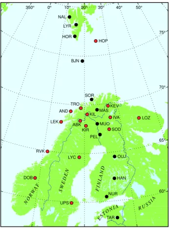
Fig. 1. IMAGE magnetometer network in 2002. Stations marked

with black dots are used in the 1-D upward continuation.

The ground-based observations have been obtained from the IMAGE magnetometers. The IMAGE array (L¨uhr et al., 1998) consists of 27 magnetometer stations maintained by 10 institutes from Estonia, Finland, Germany, Norway, Poland, Russia and Sweden. The site locations are depicted in Figure 1. For most recent information on the programme the reader is recommended to visit the IMAGE website (http://www.geo.fmi.fi/image). Together with other ground-based recordings (by radars, riometers, all-sky cameras of the MIRACLE network) and satellite observations, IMAGE is an essential part in the investigations of high-latitude magnetospheric-ionospheric physics. IMAGE evolved 1991 from the earlier EISCAT Magnetometer Cross, which was set up in 1982, and provides high-quality data useful for studies

of auroral current systems, geomagnetic induction and long-term geomagnetic activity in the auroral region. The long profile covering geographic latitudes from 58 to 79 degrees is especially favourable for auroral electrojet studies. The complete array is used in this case to compute also the spatial variation and direction of the ionospheric current densities.

The average auroral electrojets are observed mainly in a narrow region between approximately 65◦and 70◦N of

geo-magnetic latitude. They are directed anti-sunwards i.e. east-wards at dusk and westeast-wards at dawn in both hemispheres. The return currents cross the polar caps in an opposite direc-tion, from the night to the day side, and their lateral extension covers a larger region. Here, we focus on the auroral electro-jet, because the station array covers the return current only marginally.

In this paper we briefly describe the methods used to deter-mine the currents from space and from ground magnetic field data. Some typical examples show the general characteristics of the respective estimates. In chapter 4 we present a statis-tical study of the electrojet characteristics and then compare the current estimates from CHAMP and the IMAGE array for a time period of 22 months. Some selected current den-sity curves and contour maps of the results are shown. For a more quantitative comparison we perform a correlation anal-ysis and compute the amplitude ratio of the obtained current densities independently for all latitudes and for specified lo-cal time intervals. Finally we interpret the obtained results in the discussion section and compare them with earlier publi-cations.

2 Ionospheric Hall Current determined from CHAMP data

The ionospheric currents at high latitudes comprise Hall, Pedersen and field-aligned currents (FACs). All three con-tribute to the magnetic fields measured by satellites. Ground-based observations respond primarily to the Hall currents at these latitudes. The magnetic effects of the FACs and Ped-ersen currents cancel each other below the E region, if the ionospheric conductances are uniform (Fukushima, 1976). In order to distinguish between the different types of currents we assume the Hall currents to close entirely in the iono-sphere, whereas Pedersen currents are diverted into FACs. Under these conditions, and assuming vertical field-aligned currents, which is reasonable at high latitudes, only Hall cur-rents contribute to the total field and can be determined from the scalar magnetic data of the Overhauser magnetometer on CHAMP. This topic will be addressed in more detail in the discussion section.

For the estimation of the electric current density from sin-gle satellite magnetic field measurements the geometry of the current has to be known. We assume that in the polar regions the Hall currents can be approximated by a series of infinite line currents. This method has been developed and tested with Magsat and Ørsted data (Olsen, 1996), (Moretto et al., 2002). For our computations the line currents are placed at a

Fig. 1. IMAGE magnetometer network in 2002. Stations marked

with black dots are used in the 1-D upward continuation.

performs more than 15 orbits each day. During the first two years the average height above the Earth’s surface decreased from 455 km to 400 km. This time window, August 2000– May 2002, is chosen for a comparison of ground/satellite re-sults. The drift of the orbit plane in local time (LT) is about 3 h per month. Consequently, the LT of the ascending node of the orbit moved through 24 h twice in those 22 months. As the period for repeat orbits is approximately 3 days during that time, the satellite passed the region chosen for the com-parison with ground magnetometers at least twice in 72 h, alternately on ascending and descending tracks.

The ground-based observations have been obtained from the IMAGE magnetometers. The IMAGE array (L¨uhr et al., 1998) consists of 27 magnetometer stations maintained by 10 institutes from Estonia, Finland, Germany, Norway, Poland, Russia and Sweden. The site locations are depicted in Fig. 1. For the most recent information on the programme the reader is recommended to visit the IMAGE website (http://www.geo.fmi.fi/image). Together with other ground-based recordings (by radars, riometers, all-sky cameras of the MIRACLE network) and satellite observations, IMAGE is an essential part in the investigations of high-latitude magnetospheric-ionospheric physics. IMAGE evolved in 1991 from the earlier EISCAT Magnetometer Cross, which was set up in 1982, and provides high-quality data useful

for studies of auroral current systems, geomagnetic induc-tion and long-term geomagnetic activity in the auroral re-gion. The long profile covering geographic latitudes from 58 to 79 degrees is especially favourable for auroral elec-trojet studies. The complete array is used in this case to also compute the spatial variation and direction of the iono-spheric current densities. The average auroral electrojets are observed mainly in a narrow region between approximately 65◦ and 70◦N of geomagnetic latitude. They are directed anti-sunwards, i.e. eastwards at dusk and westwards at dawn, in both hemispheres. The return currents cross the polar caps in an opposite direction, from the night to the dayside, and their lateral extension covers a larger region. Here, we focus on the auroral electrojet, because the station array covers the return current only marginally.

In this paper we briefly describe the methods used to deter-mine the currents from space and from ground magnetic field data. Some typical examples show the general characteristics of the respective estimates. In Sect. 4 we present a statisti-cal study of the electrojet characteristics and then compare the current estimates from CHAMP and the IMAGE array for a time period of 22 months. Some selected current den-sity curves and contour maps of the results are shown. For a more quantitative comparison we perform a correlation anal-ysis and compute the amplitude ratio of the obtained current densities independently for all latitudes and for specified lo-cal time intervals. Finally, we interpret the obtained results in the discussion section and compare them with earlier pub-lications.

2 Ionospheric Hall Current determined from CHAMP data

The ionospheric currents at high latitudes comprise Hall, Pedersen and field-aligned currents (FACs). All three con-tribute to the magnetic fields measured by satellites. Ground-based observations respond primarily to the Hall currents at these latitudes. The magnetic effects of the FACs and Ped-ersen currents cancel each other below the E-region, if the ionospheric conductances are uniform (Fukushima, 1976). In order to distinguish between the different types of currents, we assume the Hall currents to close entirely in the iono-sphere, whereas Pedersen currents are diverted into FACs. Under these conditions, and assuming vertical field-aligned currents, which is reasonable at high latitudes, only Hall cur-rents contribute to the total field and can be determined from the scalar magnetic data of the Overhauser magnetometer on CHAMP. This topic will be addressed in more detail in the Discussion section.

For the estimation of the electric current density from sin-gle satellite magnetic field measurements the geometry of the current has to be known. We assume that in the polar regions the Hall currents can be approximated by a series of infinite line currents. This method has been developed and tested with Magsat and Ørsted data (Olsen, 1996; Moretto et al., 2002). For our computations the line currents are placed at

(4)

P. Ritter et al.: Ionospheric currents from satellite and ground 419 a height of 110 km and they are separated by 1◦ _{in latitude}

over an interval of ±80◦_{, centered at the closest approach}

of the satellite track to the geographic pole. Olsen’s method (1996) additionally includes mirror currents to simulate in-duction effects; this issue is discussed further in the Discus-sion section. The magnetic field at orbital altitude caused by an eastward directed line current can be written as

bx= − µ0I 2π h x2₊_h2, bz= − µ0I 2π x x2₊_h2, (1)

where bx and bz are the northward and downward

compo-nents of the generated magnetic field, respectively. I is the current strength, µ0is the susceptibility of free space, h

de-notes the height above the current and x is the northward dis-placement of the measurement point. The magnetic signature of the current in the field magnitude can be represented as

1F = |B + b| − |B|, (2)

where B is the unperturbed ambient magnetic field in a cor-rected geomagnetic coordinate system. Since b is much smaller than B, it is justified to replace Eq. (2) by the nor-malized dot-product between B and b

1F = B · b

|B| . (3)

With this equation we obtain a linear relation between the to-tal field deflection and the current strength, I . The intensity of each of the 160 line currents considered for the modelling can be derived from an inversion of the observed field resid-uals using a least-square-fitting approach.

For these calculations a static current system is assumed. Since CHAMP crosses the region at a speed of 4◦per minute, a certain smoothing occurs. At the orbital altitude, some 300 km above the atmosphere, we have a correlation length for a line current (here defined as the distance x from the current centre to the location where bz/bxo =0.25) of about

±1000 km. This corresponds to an averaging effect of ap-proximately 5 min.

For the inversion the magnetic data over a 160◦wide or-bit segment are used. The scalar magnetic field readings are available at a rate of 1 Hz, which is equivalent to 16 measure-ments per degree of latitude. In order to isolate the magnetic effect of the currents in the CHAMP measurements, the con-tributions from all other sources have to be subtracted from the scalar field readings. The main field is removed with the help of the recent CO2 model (Holme et al., 2003) employed up to degree and order 14. The lithospheric magnetisation is accounted for by subtracting the recent model by Maus et al. (2002). To eliminate the ring current effect, a DST

cor-rection, according to Olsen (2002), is applied. Additionally, linear trends over the entire orbital arc are removed, to avoid effects due to asymmetric ring current distributions on the day and nightsides. To suppress any currents showing up spuriously at lower magnetic latitudes (θm < 40◦), we

ap-plied a parabolic damping of the current density at the edges of the interval.

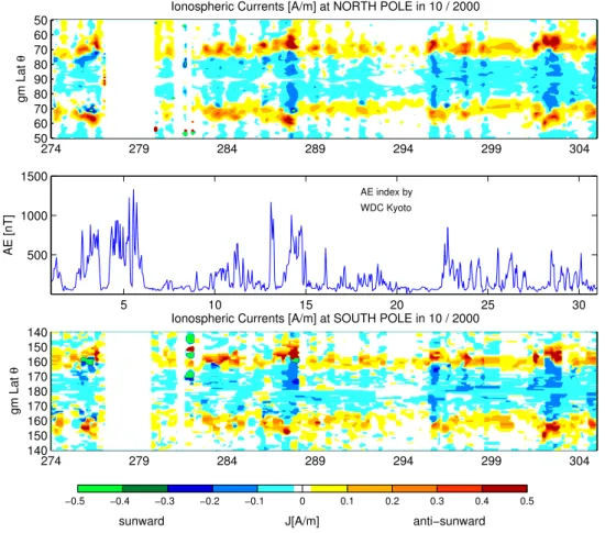
Figure 2 shows as an example of current estimates in the polar regions of the Northern and Southern Hemispheres over a period of 1 month. During that time, in October 2000, CHAMP was in a dawn/dusk orbit, thus crossing the auroral electrojets almost perpendicularly. The displayed time inter-val includes all 31 days of the month. The satellite tracks can be imagined as crossing the contour plots from top to bottom for each orbit. The auroral electrojets are prominent along two ribbons of enhanced current density at magnetic latitudes of about ±70◦. The positive amplitudes mark anti-sunward directed currents. The currents in the polar cap region are weaker and directed oppositely, from the night to the day-side, as expected. Strength and latitudinal extension of the current flow are correlated in general with the amplitudes of the AE index.

In the subauroral regions (equatorwards of the auroral electrojets) the amplitude levels of the currents are small. At these latitudes a systematic difference for dawn and dusk is evident, as indicated by the light blue and yellow colors, re-spectively. This is not an edge effect of the model, since the considered orbit arcs are much longer than those shown in the contour plots and tapering is applied at the ends. The systematic difference in amplitude is rather a hint to a non-sufficient, standard DST correction, which does not take into

account the asymmetric ring current.

3 Analysis methods for IMAGE data

The simplest way to explain variations of the ground mag-netic field is to assume that ionospheric currents flow in a fixed direction, for example, transverse to a magnetometer chain. Then it is possible to determine the ionospheric sur-face current density using the component of the field which is aligned with the chain. Typically, the auroral electrojet cur-rent flow is assumed to be in the east-west direction, and then the northward component of the field is used. We applied in this study the method based on the Fourier expansion to con-tinue the field observed on the ground to the ionospheric level (Mersmann et al., 1979).

Two-dimensional equivalent currents can be determined with the method of spherical elementary current systems, as derived by Amm and Viljanen (1999), and validated in de-tail by Pulkkinen et al. (2003). In that case we obtain both the northward and eastward components of the surface cur-rent density at ionospheric level. Because IMAGE is quite a dense array, we could always use the 2-D method, but for reference we applied the 1-D approach to show that it is also often reasonable. The 1-D method is also of importance, if the same approach is to be carried out in an area where there is only a 1-D chain of stations available (for example, Green-land).

Induction effects due to the conducting Earth could be included by setting up an additional current system below the Earth’s surface, but this is omitted here. We are mostly interested in disturbed events, and then the primary iono-spheric contribution to horizontal magnetic variations close

(5)

420 4 P. Ritter et al.: Ionospheric currents from satellite and groundRitter et al.: Ionospheric currents from satellite and ground

−0.5 −0.4 −0.3 −0.2 −0.1 0 0.1 0.2 0.3 0.4 0.5

sunward J[A/m] anti−sunward

274 279 284 289 294 299 304 50 60 70 80 90 80 70 60 50 gm Lat θ

Ionospheric Currents [A/m] at NORTH POLE in 10 / 2000

5 10 15 20 25 30 500 1000 1500 AE [nT] AE index by WDC Kyoto 274 279 284 289 294 299 304 140 150 160 170 180 170 160 150 140 gm Lat θ

Ionospheric Currents [A/m] at SOUTH POLE in 10 / 2000

Fig. 2. Ionospheric currents in the polar regions of the northern and southern hemispheres (θm: geomagnetic latitudes). For comparison the

AE index is plotted in the middle panel. The horizontal scale spans one month, given as day numbers in MJD2000 format, i.e. the Modified Julian Days are counted from 01.01.2000, 0:00:00 UT.

to electrojet centres may be about 80 % of the total varia-tion (Tanskanen et al., 2001). Neglecting inducvaria-tion means that the ground-based observations provide slightly overes-timated amplitudes of equivalent currents, but the geometric pattern of the current systems remain practically unchanged. Before determining ionospheric currents from the ground-based observations, contributions from all other field sources have to be removed. For this study a particular effort was undertaken to derive reliable base values for all the stations. We used two criteria to select quiet days for the baseline de-termination. First, the global Kpindex must be equal or less

than 1+ during the last three hours of the day. Second, the lo-cal AE index derived from IMAGE data during the last two hours of the day has to be less than 100 nT. There are 202 days fulfilling both conditions in the period January 2000 to May 2002.

After correcting some instrumental effects on magnetic

readings during this period (e.g. recalibrations of the mag-netometers or installations of new instruments), the secular variation correction is accounted for by the global satellite magnetic field model CO2 (Holme et al., 2003). No visible long term trend (< 2 nT per year) was left after that. Finally, a linear correlation between the Dst index and the field val-ues seemed to exist somewhat different for each station. A Dstcorrection thus derived was applied. The resulting base-line value Bbaseat time t is

Bbase(t) = B0+ CSV · t + CDst· Dst + f (t) (4)

where t is counted in days from Jan 1, 2000 (00:00 UT), B0

is the baseline value at t = 0, CSV is the secular variation

coefficient taken from the CO2 model, and CDstis the Dst

coefficient. Due to intentional baseline changes or due to instrumental malfunctions, an additional, individual correc-tion term f(t) is necessary at some stacorrec-tions. A check was

Fig. 2. Ionospheric currents in the polar regions of the Northern and Southern Hemispheres. For comparison the AE index is plotted in

the middle panel. The horizontal time scale spans one month, given as day numbers in MJD2000 format, i.e. the Modified Julian Days are counted from 01.01.2000, 0:00:00 UT.

to electrojet centres may be about 80% of the total varia-tion (Tanskanen et al., 2001). Neglecting inducvaria-tion means that the ground-based observations provide slightly overes-timated amplitudes of equivalent currents, but the geometric pattern of the current systems remains practically unchanged. Before determining ionospheric currents from the ground-based observations, contributions from all other field sources have to be removed. For this study a particular effort was undertaken to derive reliable base values for all the stations. We used two criteria to select quiet days for the baseline de-termination. First, the global Kpindex must be equal or less

than 1+ during the last three hours of the day. Second, the lo-cal AE index derived from IMAGE data during the last two hours of the day has to be less than 100 nT. There are 202 days fulfilling both conditions in the period January 2000 to May 2002.

After correcting some instrumental effects on magnetic readings during this period (e.g. recalibrations of the mag-netometers or installations of new instruments), the secular variation correction is accounted for by the global satellite magnetic field model CO2 (Holme et al., 2003). No visible longterm trend (< 2 nT per year) was left after that. Finally, a linear correlation between the Dst index and the field values

seemed to exist, somewhat different for each station. A Dst

correction thus derived was applied. The resulting baseline value Bbaseat time t is

Bbase(t ) =B0+CSV ·t +CDst ·Dst+f (t), (4)

where t is counted in days from 1 January 2000 (00:00 UT),

B0is the baseline value at t = 0, CSV is the secular

varia-tion coefficient taken from the CO2 model, and CDst is the

Dst coefficient. Due to intentional baseline changes or due

to instrumental malfunctions, an additional, individual cor-rection term f (t ) is necessary at some stations. A check was made excluding some stations with outliers not covered by f (t ). A more detailed description of the baseline deter-mination method and correction terms f (t ) can be found in Sillanp¨a¨a et al. (2003). A visual inspection of the field sig-natures showed that the automatic baseline selection is rea-sonable, if the magnetic effects caused by the currents are at least several tens of nT.

For 1-D equivalent current estimates, Bxfrom the stations

along the chain TAR-NAL in Fig. 1 can be used (TAR started to operate in September 2001, and it was not considered here). Equivalent current densities were given at the height of 100 km along a geographic meridian from about 60◦to 79◦

(6)

P. Ritter et al.: Ionospheric currents from satellite and ground 421

Ritter et al.: Ionospheric currents from satellite and ground 5

made excluding some stations with outliers not covered by f (t). A more detailed description of the baseline determina-tion method and correcdetermina-tion terms f(t) can be found in Sil-lanp¨a¨a et al. (2003). A visual inspection of the field signa-tures showed that the automatic baseline selection is reason-able, if the magnetic effects caused by the currents are at least several tens of nT.

For 1-D equivalent current estimates, Bxfrom the stations

along the chain TAR-NAL in Figure 1 can be used (TAR started to operate in September 2001, and it was not con-sidered here). Equivalent current densities were given at the height of 100 km along a geographic meridian from about 60◦to 79◦geographic latitude with a spacing of about 0.7◦.

This meridian is not precisely aligned with the magnetome-ter chain, but it can be imagined to cross the central parts of IMAGE. Due to the 1-D assumption the zonal location of the meridian does not matter.

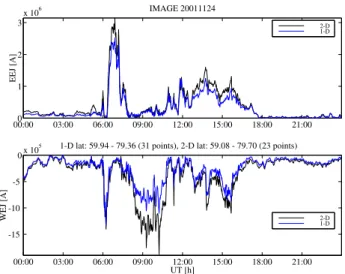
00:000 03:00 06:00 09:00 12:00 15:00 18:00 21:00 1 2 3x 10 6 EEJ [A] IMAGE 20011124 2-D 1-D 00:00 03:00 06:00 09:00 12:00 15:00 18:00 21:00 -15 -10 -5 0x 10 5 UT [h] WEJ [A]

1-D lat: 59.94 - 79.36 (31 points), 2-D lat: 59.08 - 79.70 (23 points)

2-D 1-D

Fig. 3. Total eastward and westward electrojet equivalent

iono-spheric currents over IMAGE on 24 November 2001. The blue curve corresponds to the 1-D upward continuation, whereas the black curve shows the result by the 2-D method of spherical ele-mentary current systems.

For the 2-D equivalent current estimates, we used a set of about 1600 elementary current systems at a height of 100 kmin a regular grid (54◦_{− 84}◦N, 2.5◦_{− 42.5}◦E)

cover-ing the whole IMAGE array with a sufficient outward exten-sion. Amplitudes of the elements were determined by using the horizontal components Bx and By of all available

IM-AGE sites. We considered CHAMP footpoints in the area of 60◦_{− 78}◦N and 10◦_{− 30}◦E, where edge effects do not cause

artefacts.

Although at certain times 1-D and 2-D equivalent currents may be quite different, the overall agreement is reasonably good, as shown in Figure 3. The total amplitudes of the elec-trojets are underestimated by the 1-D method.

This can be understood when considering the horizontal magnetic field of a line current of finite length with vertical currents at both ends. Assume for simplicity that the observa-tion point is just below the centre of the horizontal segment.

Keeping the amplitude of the current fixed, but increasing the length of the horizontal part, the horizontal field increases, as can be easily deduced by applying the Biot-Savart law. Con-sequently, the 1-D method underestimates the amplitudes, because real currents are never infinitely long. However, at times the electrojet seems to be very long, as around 06 UT for the WEJ case in Figure 3, where both methods yield very much the same total current.

4 Comparison of satellite and ground based measure-ments

After having presented the techniques for estimating iono-spheric Hall currents both from space and from ground we will apply them for auroral current studies.

4.1 An event study

We are going to inspect an active period. As an example we selected the strong magnetic storm of 5/6 Nov. 2001. It reached DST values of -277 nT. The storm commences, as

can be seen on Figure 4, shortly after 20 UT on 5 Nov. The event start is also evident from the decrease of DST. The

tual main phase, however, starts only on the next morning ac-companied by a large SSC at 01:53 UT. The electrojet centre moves as far south as 58◦ around 03 UT. During the

subse-quent hours the auroral electrojet retracts poleward reaching 68◦ at 05 UT. The activity stays high until 06 UT reaching

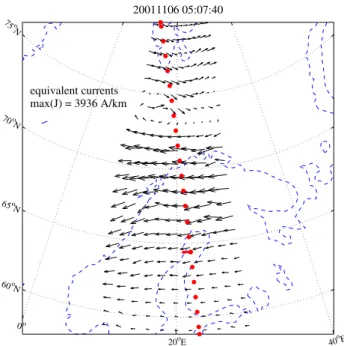
amplitudes of up to 2400 nT and decays only after that time. At about 05:07 UT CHAMP passed the IMAGE array from north to south (dashed vertical line in Figure 4). At that time the magnetic field is still strongly deflected. Fig-ure 5 shows the equivalent current distribution as derived by the 2-D method for the time of the CHAMP overflight. There are very strong westward currents, reaching almost 4 A/m in northern Scandinavia. Poleward of Bear Island we find weaker eastward currents. A direct comparison be-tween the ground and satellite estimates is presented in Fig-ure 6. The blue curve represents current densities derived from ground-based data and the red currents denote those from satellite readings. Both curves track each other quite closely. Ground-based estimates are slightly higher, on aver-age by 15%.

In the same diagram we also show the field aligned cur-rents (FACs) estimated from CHAMP magnetic field vector data. For this coarse comparison we have assumed infinite FAC-sheets perpendicular to the flight direction. Poleward of 74◦N there are no significant FACs. Further south we find a

distinct downward current region. When going equatorward a series of up- and downward FAC sheets follows where the upward flow gradually starts to dominate.

Combining all these measurements we get a rather consis-tent picture of the morning side polar convection cell. The downward FACs at 72◦N can be associated with the Region

1 currents. Poleward we find the weaker polar cap eastward (sunward) currents. Equatorward there is the very intense

Fig. 3. Total eastward and westward electrojet equivalent

iono-spheric currents over IMAGE on 24 November 2001. The blue curve corresponds to the 1-D upward continuation, whereas the black curve shows the result by the 2-D method of spherical ele-mentary current systems.

geographic latitude with a spacing of about 0.7◦. This merid-ian is not precisely aligned with the magnetometer chain, but it can be imagined to cross the central parts of IMAGE. Due to the 1-D assumption, the zonal location of the meridian does not matter.

For the 2-D equivalent current estimates, we used a set of about 1600 elementary current systems at a height of 100 km in a regular grid (54◦–84◦N, 2.5◦–42.5◦E) cover-ing the whole IMAGE array with a sufficient outward exten-sion. Amplitudes of the elements were determined by using the horizontal components Bx and By of all available

IM-AGE sites. We considered CHAMP footpoints in the area of 60◦_–78◦_{N and 10}◦_–30◦_{E, where edge effects do not cause}

artifacts.

Although at certain times 1-D and 2-D equivalent currents may be quite different, the overall agreement is reasonably good, as shown in Fig. 3. The total amplitudes of the elec-trojets are underestimated by the 1-D method. This can be understood when considering the horizontal magnetic field of a line current of finite length with vertical currents at both ends. Assume for simplicity that the observation point is just below the centre of the horizontal segment. Keeping the am-plitude of the current fixed, but increasing the length of the horizontal part, the horizontal field increases, as can be easily deduced by applying the Biot-Savart law. Consequently, the 1-D method underestimates the amplitudes, because real cur-rents are never infinitely long. However, at times, the elec-trojet seems to be very long, as around 06:00 UT for the WEJ case in Fig. 3, where both methods yield very much the same total current.

IMAGE magnetometer network 2001-11-05

16 22 04 10 Hour (UT) X-COMPONENT 4000 nT 1 minute averages NAL LYR HOR BJN SOR MAS MUO PEL OUJ HAN NUR TAR

Fig. 4. Magnetograms of the IMAGE stations (for locations refer

to Figure 1) of the storm event starting on 5 November 2001; Bx

component. 20011106 05:07:40 0o 20oE 40oE 60o_N 65o N 70o N 75 o N equivalent currents max(J) = 3936 A/km

Fig. 5. Snapshot of equivalent currents on 6 November 2001,

de-termined by IMAGE (black arrows) and CHAMP footprints (red dots).

westward auroral electrojet. The transition from the Region 1 to the Region 2 occurs overhead the auroral electrojet and is characterized by alternating upward and downward FACs.

This signature suggests that the plasma convection in the magnetosphere is not entirely laminar but may form vortices at the interface between tailward and sunward flows. Con-sequently, we find the most intense upward FACs not in the Region 2 proper but overhead the auroral electrojet, giving probably rise to a high conductivity.

55 60 65 70 75 80 −10 −5 0 5 j [A/m]

Hall Currents and FACs above IMAGE Region, dsc.

MJD 675.2, orbit #07383 2001/11/06 at 5:06 (60°)

geogr. latitude θ [deg]

CHAMP OVM IMAGE 2−D

FACs (10sec) [A/km2_]

Fig. 6. Hall currents and field-aligned currents (10 sec running

mean) during the storm event on 5/6 Nov. 2001

The size of the polar cap is not particularly large during the inspected passage. The boundary marked by the convection reversal in Figure 5 occurs at about 70◦magnetic latitude (at

the IMAGE region corrected magnetic latitudes are about 3◦

lower than geographic ones). At the time of the main phase of the storm (03 UT) the boundary is 10◦further south. This

implies a polar cap with a radius of 30◦. The resulting

mag-netic flux stored in the tail during that time is therefore about 4 times higher than normal. The release of this magnetic en-ergy causes the very intense currents.

4.2 A statistical study

During a period of 22 months we identified 490 satellite over-flights across the region of the IMAGE magnetometer array. The ionospheric currents were determined from CHAMP data and independently computed from the ground-based measurements using the 2D method, as described above. The full set of stations supplied the database for the 2D approach. Figure 7 shows the current density profiles of 16 overflights as examples. The agreement of the curves is good in general, indicating that the signatures of the ionospheric currents in the magnetic field can be detected equally clear on ground and at satellite heights.

Current density profiles for all overflight events during the time period MJD 215 - MJD 880 (Modified Julian Days) are shown in Figure 8, sorted by ascending and descend-ing tracks on the left and right side, respectively. Therefore, the magnetic local times scales (MLT) of the left and right frames differ by 12 h, and accordingly, the derived currents have predominantly opposite signs. Positive currents (yel-low and red) are directed eastward, whereas negative (blue and green) currents flow westward.

Currents determined from CHAMP magnetic field data are displayed at the top, those from the IMAGE stations are pre-sented in the bottom frames. During periods of increased ac-tivity the current estimates are generally in good agreement, the coincidence of the prominent amplitude maxima is ob-vious. The light-blue band (with J ≈ −0.1 A/m) visible

Fig. 4. Magnetograms of the IMAGE stations (for locations refer to

Fig. 1) of the storm event starting on 5 November 2001; Bx

compo-nent.

4 Comparison of satellite and ground-based measure-ments

After having presented the techniques for estimating iono-spheric Hall currents, both from space and from ground, we will apply them for auroral current studies.

4.1 An event study

We are going to inspect an active period. As an example we selected the strong magnetic storm of 5/6 November 2001. It reached DST values of −277 nT. The storm commences, as

can be seen in Fig. 4, shortly after 20:00 UT on 5 Novem-ber. The event start is also evident from the decrease of

DST. The actual main phase, however, starts only on the

next morning, accompanied by a large SSC at 01:53 UT. The electrojet centre moves as far south as 58◦around 03:00 UT. During the subsequent hours, the auroral electrojet retracts poleward, reaching 68◦at 05:00 UT. The activity stays high until 06:00 UT, reaching amplitudes of up to 2400 nT and decays only after that time.

At about 05:07 UT CHAMP passed the IMAGE array from north to south (dashed vertical line in Fig. 4). At that time the magnetic field is still strongly deflected. Figure 5 shows the equivalent current distribution as derived by the

(7)

422 P. Ritter et al.: Ionospheric currents from satellite and ground

IMAGE magnetometer network 2001-11-05

16 22 04 10 Hour (UT) X-COMPONENT 4000 nT 1 minute averages NAL LYR HOR BJN SOR MAS MUO PEL OUJ HAN NUR TAR

Fig. 4. Magnetograms of the IMAGE stations (for locations refer

to Figure 1) of the storm event starting on 5 November 2001; Bx

component. 20011106 05:07:40 0o 20oE 40oE 60o_N 65o_N 70_o N 75_o N equivalent currents max(J) = 3936 A/km

westward auroral electrojet. The transition from the Region 1 to the Region 2 occurs overhead the auroral electrojet and is characterized by alternating upward and downward FACs.

This signature suggests that the plasma convection in the magnetosphere is not entirely laminar but may form vortices at the interface between tailward and sunward flows. Con-sequently, we find the most intense upward FACs not in the Region 2 proper but overhead the auroral electrojet, giving probably rise to a high conductivity.

55 60 65 70 75 80 −10 −5 0 5 j [A/m]

MJD 675.2, orbit #07383 2001/11/06 at 5:06 (60°) geogr. latitude θ [deg]

CHAMP OVM IMAGE 2−D

FACs (10sec) [A/km2_]

Fig. 6. Hall currents and field-aligned currents (10 sec running

mean) during the storm event on 5/6 Nov. 2001

The size of the polar cap is not particularly large during the inspected passage. The boundary marked by the convection reversal in Figure 5 occurs at about 70◦magnetic latitude (at the IMAGE region corrected magnetic latitudes are about 3◦ lower than geographic ones). At the time of the main phase of the storm (03 UT) the boundary is 10◦further south. This implies a polar cap with a radius of 30◦. The resulting mag-netic flux stored in the tail during that time is therefore about 4 times higher than normal. The release of this magnetic en-ergy causes the very intense currents.

During a period of 22 months we identified 490 satellite over-flights across the region of the IMAGE magnetometer array. The ionospheric currents were determined from CHAMP data and independently computed from the ground-based measurements using the 2D method, as described above. The full set of stations supplied the database for the 2D approach. Figure 7 shows the current density profiles of 16 overflights as examples. The agreement of the curves is good in general, indicating that the signatures of the ionospheric currents in the magnetic field can be detected equally clear on ground and at satellite heights.

Current density profiles for all overflight events during the time period MJD 215 - MJD 880 (Modified Julian Days) are shown in Figure 8, sorted by ascending and descend-ing tracks on the left and right side, respectively. Therefore, the magnetic local times scales (MLT) of the left and right frames differ by 12 h, and accordingly, the derived currents have predominantly opposite signs. Positive currents (yel-low and red) are directed eastward, whereas negative (blue and green) currents flow westward.

Currents determined from CHAMP magnetic field data are displayed at the top, those from the IMAGE stations are pre-sented in the bottom frames. During periods of increased ac-tivity the current estimates are generally in good agreement, the coincidence of the prominent amplitude maxima is ob-vious. The light-blue band (with J ≈ −0.1 A/m) visible

2-D method for the time of the CHAMP overflight. There are very strong westward currents, reaching almost 4 A/m in northern Scandinavia. Poleward of Bear Island we find weaker eastward currents. A direct comparison between the ground and satellite estimates is presented in Fig. 6. The blue curve represents current densities derived from ground-based data and the red currents denote those from satellite readings. Both curves track each other quite closely. Ground-based es-timates are slightly higher, on average by 15%.

In the same diagram we also show the field-aligned cur-rents (FACs) estimated from CHAMP magnetic field vector data. For this coarse comparison we have assumed infinite FAC-sheets perpendicular to the flight direction. Poleward of 74◦N there are no significant FACs. Further south we find a distinct downward current region. When going equatorward a series of up- and downward FAC sheets follows where the upward flow gradually starts to dominate.

By combining all these measurements we obtain a rather consistent picture of the morning side polar convection cell. The downward FACs at 72◦_{N can be associated with the}

Region 1 currents. Poleward we find the weaker polar cap eastward (sunward) currents. Equatorward there is the very intense westward auroral electrojet. The transition from the Region 1 to the Region 2 occurs above the auroral electro-jet and is characterized by alternating upward and downward FACs. This signature suggests that the plasma convection in the magnetosphere is not entirely laminar but may form vortices at the interface between tailward and sunward flows. Consequently, we find the most intense upward FACs not in the Region 2 proper but above the auroral electrojet, giving probably rise to a high conductivity.

The size of the polar cap is not particularly large during the inspected passage. The boundary marked by the convection reversal in Fig. 5 occurs at about 70◦ _{magnetic latitude (at}

the IMAGE region corrected magnetic latitudes are about 3◦ lower than geographic ones). At the time of the main phase of the storm (03:00 UT) the boundary is 10◦ further south. This implies a polar cap with a radius of 30◦. The resulting magnetic flux stored in the tail during that time is, therefore, about 4 times higher than normal. The release of this mag-netic energy causes the very intense currents.

During a period of 22 months, we identified 490 satellite overflights across the region of the IMAGE magnetome-ter array. The ionospheric currents were demagnetome-termined from CHAMP data and independently computed from the ground-based measurements using the 2-D method, as described above. The full set of stations supplied the database for the 2-D approach. Figure 7 shows the current density profiles of 16 overflights as examples. The agreement of the curves is good in general, indicating that the signatures of the iono-spheric currents in the magnetic field can be detected equally clear on the ground and at satellite heights.

Current density profiles for all overflight events during the time period MJD 215–MJD 880 (Modified Julian Days) are shown in Fig. 8, sorted by ascending and descending tracks on the left and right side, respectively. Therefore, the mag-netic local times scales (MLT) of the left and right frames differ by 12 h, and accordingly, the derived currents have pre-dominantly opposite signs. Positive currents (yellow and red) are directed eastward, whereas negative (blue and green) cur-rents flow westward.

Currents determined from CHAMP magnetic field data are displayed at the top, and those from the IMAGE stations are presented in the bottom frames. During periods of increased activity, the current estimates are generally in good agree-ment, and the coincidence of the prominent amplitude max-ima is obvious. The light-blue band (with J ≈ − 0.1 A/m), visible around 65◦ in the satellite data, is presumably due to short-scale crustal magnetic features in the Kiruna area, which are not resolved and removed completely by the litho-spheric model used for our crustal correction.

The latitudinal displacement of the mean current locations with local time is clearly visible: around noon they are re-tracted poleward by several degrees, whereas shortly before midnight they reach their most equatorward position.

Besides the local time dependencies there are marked sea-sonal effects. During the winter solstice, the average activ-ity is strongly reduced. This fact is particularly evident in the morning up to pre-noon hours. In our survey this time sector was sampled during winter months on days around MJD 760 by ascending tracks and around MJD 380 by de-scending tracks. For a period of almost 90 days the current densities hardly exceed the noise level. We find around mid-night in winter individual storm/substorm events (MJD 350

(8)

P. Ritter et al.: Ionospheric currents from satellite and ground 423

6 Ritter et al.: Ionospheric currents from satellite and ground

IMAGE magnetometer network 2001-11-05

16 22 04 10 Hour (UT)

X-COMPONENT

4000 nT 1 minute averages NAL LYR HOR BJN SOR MAS MUO PEL OUJ HAN NUR TAR

Fig. 4. Magnetograms of the IMAGE stations (for locations refer

to Figure 1) of the storm event starting on 5 November 2001; B

x

component.

20011106 05:07:40

0

o

20

o

E

₄₀

o

E

60

o

_N

65

o

N

70

_o

N

75

o

N

equivalent currents

max(J) = 3936 A/km

Fig. 5. Snapshot of equivalent currents on 6 November 2001,

de-termined by IMAGE (black arrows) and CHAMP footprints (red

dots).

westward auroral electrojet. The transition from the Region

1 to the Region 2 occurs overhead the auroral electrojet and

is characterized by alternating upward and downward FACs.

This signature suggests that the plasma convection in the

magnetosphere is not entirely laminar but may form vortices

at the interface between tailward and sunward flows.

Con-sequently, we find the most intense upward FACs not in the

Region 2 proper but overhead the auroral electrojet, giving

probably rise to a high conductivity.

55 60 65 70 75 80 −10 −5 0 5 j [A/m]

MJD 675.2, orbit #07383 2001/11/06 at 5:06 (60°)

CHAMP OVM IMAGE 2−D FACs (10sec) [A/km2]

Fig. 6. Hall currents and field-aligned currents (10 sec running

mean) during the storm event on 5/6 Nov. 2001

The size of the polar cap is not particularly large during the

inspected passage. The boundary marked by the convection

reversal in Figure 5 occurs at about 70

◦

magnetic latitude (at

the IMAGE region corrected magnetic latitudes are about 3

◦

lower than geographic ones). At the time of the main phase

of the storm (03 UT) the boundary is 10

◦

further south. This

implies a polar cap with a radius of 30

◦

. The resulting

mag-netic flux stored in the tail during that time is therefore about

4 times higher than normal. The release of this magnetic

en-ergy causes the very intense currents.

4.2 A statistical study

During a period of 22 months we identified 490 satellite

over-flights across the region of the IMAGE magnetometer array.

The ionospheric currents were determined from CHAMP

data and independently computed from the ground-based

measurements using the 2D method, as described above. The

full set of stations supplied the database for the 2D approach.

Figure 7 shows the current density profiles of 16 overflights

as examples. The agreement of the curves is good in general,

indicating that the signatures of the ionospheric currents in

the magnetic field can be detected equally clear on ground

and at satellite heights.

Current density profiles for all overflight events during the

time period MJD 215 - MJD 880 (Modified Julian Days)

are shown in Figure 8, sorted by ascending and

descend-ing tracks on the left and right side, respectively. Therefore,

the magnetic local times scales (MLT) of the left and right

frames differ by 12 h, and accordingly, the derived currents

have predominantly opposite signs. Positive currents

(yel-low and red) are directed eastward, whereas negative (blue

and green) currents flow westward.

Currents determined from CHAMP magnetic field data are

displayed at the top, those from the IMAGE stations are

pre-sented in the bottom frames. During periods of increased

ac-tivity the current estimates are generally in good agreement,

the coincidence of the prominent amplitude maxima is

ob-vious. The light-blue band (with J ≈ −0.1 A/m) visible

Fig. 6. Hall currents and field-aligned currents (10-s running mean) during the storm event on 5/6 Nov. 2001.

Ritter et al.: Ionospheric currents from satellite and ground

7

−0.5 0 0.5

j [A/m]

Hall Currents above IMAGE Region, asc.

MJD 338.0 # 00292 2000/12/04 at 0:32 −0.5 0 0.5 _{MJD 357.9 # 00338} 2000/12/23 at 22:45 −0.5 0 0.5 _{MJD 391.8 # 00384} 2001/01/26 at 19:37 −0.5 0 0.5 _{MJD 413.7 # 00430} 2001/02/17 at 17:49 −0.5 0 0.5 _{MJD 627.9 # 00476} 2001/09/19 at 22:35 −0.5 0 0.5 _{MJD 635.9 # 00491} 2001/09/27 at 21:32 −0.5 0 0.5 _{MJD 667.8 # 00522} 2001/10/29 at 18:33 55 60 65 70 75 80 −0.5 0 0.5 _{MJD 863.0 # 00537} 2002/05/13 at 0:32

−0.5 0 0.5

j [A/m]

Hall Currents above IMAGE Region, dsc.

MJD 228.9 # 00299 2000/08/16 at 21:19 −0.5 0 0.5 _{MJD 282.7 # 00345} 2000/10/09 at 16:45 −0.5 0 0.5 _{MJD 309.6 # 00391} 2000/11/05 at 14:10 −0.5 0 0.5 _{MJD 453.0 # 00406} 2001/03/29 at 1:09 −0.5 0 0.5 _{MJD 474.0 # 00437} 2001/04/18 at 23:33 −0.5 0 0.5 _{MJD 557.7 # 00452} 2001/07/11 at 15:50 −0.5 0 0.5 _{MJD 689.2 # 00483} 2001/11/20 at 4:01 55 60 65 70 75 80 −0.5 0 0.5 _{MJD 805.7 # 00498} 2002/03/16 at 16:57

Fig. 7. Comparison of the current densities derived from CHAMP (red lines) and IMAGE ground-based measurements (blue lines) between

Aug 2000 (MJD 215) - May 2002(MJD 880) on N/S profiles across the IMAGE array (60◦

− 80◦N geographic latitudes). Left side: the satellite crossed the region on ascending tracks; right side: on descending tracks. MJD = Modified Julian Days (format see Figure 2).

around 65

◦

in the satellite data is presumably due to

short-scale crustal magnetic features in the Kiruna area, which

are not resolved and removed completely by the lithospheric

model used for our crustal correction.

The latitudinal displacement of the mean current locations

with local time is clearly visible: around noon they are

re-tracted poleward by several degrees, whereas shortly before

midnight they reach their most equatorward position.

Besides the local time there are marked seasonal effects.

During the winter solstice the average activity is strongly

re-duced. This fact is particularly evident in the morning up

to pre-noon hours. In our survey this time sector was

sam-pled during winter months on days around MJD 760 by

as-cending tracks and around MJD 380 by desas-cending tracks.

For a period of almost 90 days the current densities hardly

exceed the noise level. Around midnight we find in winter

individual storm/substorm events (MJD 350 ascending and

MJD 730 descending), but during the time in-between there

is generally low activity.

According to Russel and McPherron (1973), equinox

sea-sons are characterized by enhanced magnetic activity. From

our observations we can confirm an increase in

substorm-related westward auroral electrojets during these seasons,

when they are sampled around midnight hours (asc.: MJD

620, 860; desc.: MJD 470). When sampled at daytime, the

Russel-McPherron effect is less pronounced. Only in one out

of four possible cases we find enhanced eastward currents

(asc.: MJD 450). During the summer solstice the eastward

currents in the afternoon sector are quite prominent (desc.:

MJD560). This is probably due to greatly enhanced

iono-spheric conductivity caused by the continuous solar

illumi-nation during this season.

Our systematic survey samples all seasons independently

of activity and thus provides an unbiased view of the auroral

electrojet current distribution.

4.3 Correlation analysis of ground/satellite results

A more quantitative measure for the agreement of the results

derived from space and ground data can be obtained, if the

properties and characteristics of the amplitude ratios of all

available overflights are analysed. For that purpose Figure 9

presents scatter plots of the CHAMP versus IMAGE current

densities at selected latitudes along the IMAGE meridional

profile. The solid lines mark the linear regressions computed

for the case where the more homogeneous satellite results

Fig. 7. Comparison of the current densities derived from CHAMP (red lines) and IMAGE ground-based measurements (blue lines) between

Aug 2000 (MJD 215) – May 2002(MJD 880) on N/S profiles across the IMAGE array (60◦–80◦N geographic latitudes). Left side: the satellite crossed the region on ascending tracks; right side: on descending tracks. MJD = Modified Julian Days (format see Fig. 2).

(9)

424₈ P. Ritter et al.: Ionospheric currents from satellite and ground_{Ritter et al.: Ionospheric currents from satellite and ground}

−1 −0.5 0 0.5

West−EJ J[A/m] East−EJ

220 310 400 490 580 670 760 850 60 65 70 75 gg Latitude

Ionospheric Currents from CHAMP Data − ascending tracks

12MLT06 24 18 12 06 24 18 12 06 220 310 400 490 580 670 760 850 60 65 70 75 MJD2000 gg Latitude

Ionospheric Currents from IMAGE Data

Autumn Winter Spring Summer Autumn Winter Spring S

220 310 400 490 580 670 760 850 60 65 70 75 gg Latitude

Ionospheric Currents from CHAMP Data − descending tracks

Fig. 8. Ionospheric currents for all 490 overflights during the time period MJD 215 - MJD 880. Upper frames: determined from CHAMP

data above the IMAGE region; lower frames: determined from IMAGE data. Left side: only ascending tracks; right side: only descending tracks. The red numbers in the top frames give the respective magnetic local times (MLT).

(y-axes) are assumed to be free of errors.

−0.5 0 0.5 −0.5 0 0.5 CHAMP [A/m] lin. correlation at θ = 77° −0.5 0 0.5 −0.5 0 0.5 CHAMP [A/m] lin. correlation at θ = 68° −0.5 0 0.5 −0.5 0 0.5 CHAMP [A/m] lin. correlation at θ = 74° −0.5 0 0.5 −0.5 0 0.5 CHAMP [A/m] lin. correlation at θ = 66° −0.5 0 0.5 −0.5 0 0.5 IMAGE−2D [A/m] CHAMP [A/m] lin. correlation at θ = 70° −0.5 0 0.5 −0.5 0 0.5 IMAGE−2D [A/m] CHAMP [A/m] lin. correlation at θ = 60°

Fig. 9. Scatter plots of the ratios of current densities at selected

latitudes determined from IMAGE and CHAMP. Linear regression lines are added.

Only few data points scatter completely away from the re-gression lines. The distribution of the ratios is clearly linear only down to ≈ 63◦N of geographic latitude. For lower

lat-itudes the current intensity becomes very small due to the rapidly decreasing conductivity.

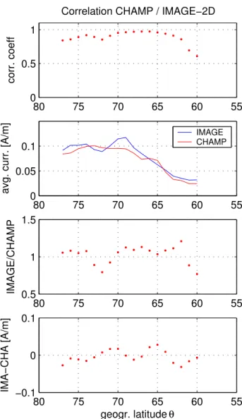
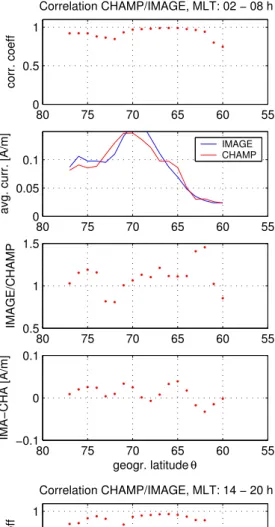
Figure 10 pictures the results of the correlation analysis determined for each degree of latitude individually. From

top to bottom the diagrams show the correlation coefficients Rc, average current densities, and the regression coefficients

of all scatter plots, namely the amplitude ratios between IM-AGE and CHAMP (inverse regression line slope) and local bias (regression line offset). These quantities were computed from the current estimates obtained over the IMAGE array in the region θ = 60◦_{... 80}◦N.

The second frame shows the average magnitude of the cur-rent densities along the profile, individually for satellite and ground-based data. The estimated current densities are fairly low on average, indicating that most of the overflights oc-curred during quiet periods. Starting from polar latitudes, the intensity obtained from CHAMP rises, attaining a plateau between θ = 74◦and 69◦N. Thereafter it drops off. Current

densities estimated from IMAGE data are generally higher. They reach a first maximum at θ = 74◦N. A second

max-imum is attained at 68◦ _{− 70}◦N. The local minimum

in-between is co-located with the station gap in-between SOR and BJN (cf. Figure 1). For θ < 68◦N the two curves fall off

gradually, reaching the noise level at 63◦N. The 2D IMAGE

results yield values that are very much the same as those ob-tained from the satellite measurements.

The correlation coefficient Rc in the top graph is close

to one. Between θ = 65◦ and 70◦N we obtain R

c =

0.96 ± 0.014. A shallow minimum occurs where we have poor ground data support over the sea. Naturally, the corre-lation drops off in the region south of the electrojet. The third graph shows a similar picture, the amplitude ratio IMAGE to CHAMP stays close to one in the region of high current den-sity. The average value for the ratio between θ = 63◦...

70◦N is 1.08 ± 0.01. The offset of the regression lines

(in-tercept), as shown in the bottom panel, may either be caused

Fig. 8. Ionospheric currents for all 490 overflights during the time period MJD 215–MJD 880. Upper frames: determined from CHAMP

data above the IMAGE region; lower frames: determined from IMAGE data. Left side: only ascending tracks; right side: only descending tracks. The red numbers in the top frames give the respective magnetic local times (MLT).

8 Ritter et al.: Ionospheric currents from satellite and ground

−1 −0.5 0 0.5

West−EJ J[A/m] East−EJ

220 310 400 490 580 670 760 850 60 65 70 75 gg Latitude

Ionospheric Currents from CHAMP Data − ascending tracks

220 310 400 490 580 670 760 850 60 65 70 75 gg Latitude

Ionospheric Currents from CHAMP Data − descending tracks

Fig. 8. Ionospheric currents for all 490 overflights during the time period MJD 215 - MJD 880. Upper frames: determined from CHAMP

data above the IMAGE region; lower frames: determined from IMAGE data. Left side: only ascending tracks; right side: only descending

tracks. The red numbers in the top frames give the respective magnetic local times (MLT).

(y-axes) are assumed to be free of errors.

−0.5 0 0.5 −0.5 0 0.5 CHAMP [A/m] lin. correlation at θ = 77° −0.5 0 0.5 −0.5 0 0.5 CHAMP [A/m] lin. correlation at θ = 68° −0.5 0 0.5 −0.5 0 0.5 CHAMP [A/m] lin. correlation at θ = 74° −0.5 0 0.5 −0.5 0 0.5 CHAMP [A/m] lin. correlation at θ = 66° −0.5 0 0.5 −0.5 0 0.5 IMAGE−2D [A/m] CHAMP [A/m] lin. correlation at θ = 70° −0.5 0 0.5 −0.5 0 0.5 IMAGE−2D [A/m] CHAMP [A/m] lin. correlation at θ = 60°

Fig. 9. Scatter plots of the ratios of current densities at selected

latitudes determined from IMAGE and CHAMP. Linear regression

lines are added.

Only few data points scatter completely away from the

re-gression lines. The distribution of the ratios is clearly linear

only down to ≈ 63

◦

N of geographic latitude. For lower

lat-itudes the current intensity becomes very small due to the

rapidly decreasing conductivity.

Figure 10 pictures the results of the correlation analysis

determined for each degree of latitude individually. From

top to bottom the diagrams show the correlation coefficients

R

c

, average current densities, and the regression coefficients

of all scatter plots, namely the amplitude ratios between

IM-AGE and CHAMP (inverse regression line slope) and local

bias (regression line offset). These quantities were computed

from the current estimates obtained over the IMAGE array in

the region θ = 60

◦

_{... 80}

◦

N. The second frame shows the average magnitude of the

cur-rent densities along the profile, individually for satellite and

ground-based data. The estimated current densities are fairly

low on average, indicating that most of the overflights

oc-curred during quiet periods. Starting from polar latitudes,

the intensity obtained from CHAMP rises, attaining a plateau

between θ = 74

◦

and 69

◦

N. Thereafter it drops off. Current

densities estimated from IMAGE data are generally higher.

They reach a first maximum at θ = 74

◦

N. A second

max-imum is attained at 68

◦

_{− 70}

◦

N. The local minimum

in-between is co-located with the station gap in-between SOR and

BJN (cf. Figure 1). For θ < 68

◦

N the two curves fall off

gradually, reaching the noise level at 63

◦

N. The 2D IMAGE

results yield values that are very much the same as those

ob-tained from the satellite measurements.

The correlation coefficient R

c

in the top graph is close

to one. Between θ = 65

◦

and 70

◦

N we obtain R

c

=

0.96 ± 0.014. A shallow minimum occurs where we have

poor ground data support over the sea. Naturally, the

corre-lation drops off in the region south of the electrojet. The third

graph shows a similar picture, the amplitude ratio IMAGE to

CHAMP stays close to one in the region of high current

den-sity. The average value for the ratio between θ = 63

◦

...

70

◦

N is 1.08 ± 0.01. The offset of the regression lines

(in-tercept), as shown in the bottom panel, may either be caused

Fig. 9. Scatter plots of the ratios of current densities at selected latitudes determined from IMAGE and CHAMP. Linear regression lines are