HAL Id: hal-00316904
https://hal.archives-ouvertes.fr/hal-00316904
Submitted on 1 Jan 2001
HAL is a multi-disciplinary open access
archive for the deposit and dissemination of
sci-entific research documents, whether they are
pub-lished or not. The documents may come from
teaching and research institutions in France or
abroad, or from public or private research centers.
L’archive ouverte pluridisciplinaire HAL, est
destinée au dépôt et à la diffusion de documents
scientifiques de niveau recherche, publiés ou non,
émanant des établissements d’enseignement et de
recherche français ou étrangers, des laboratoires
publics ou privés.
Thermospheric zonal temperature gradients observed at
low latitudes
P. R. Fagundes, Y. Sahai, J. A. Bittencourt
To cite this version:
P. R. Fagundes, Y. Sahai, J. A. Bittencourt. Thermospheric zonal temperature gradients observed
at low latitudes. Annales Geophysicae, European Geosciences Union, 2001, 19 (9), pp.1133-1139.
�hal-00316904�
Annales
Geophysicae
Thermospheric zonal temperature gradients observed at low
latitudes
P. R. Fagundes1, Y. Sahai2, and J. A. Bittencourt2
1Universidade do Vale do Paraiba / UNIVAP, Av. Shishima Hifumi, 291, CEP 12244-000, S˜ao Jos´e dos Campos, Brazil 2Instituto Nacional de Pesquisas Espaciais - INPE, CP: 514, CEP 12201-970, S˜ao Jos´e dos Campos, Brazil
Received: 16 October 2000 – Revised: 8 June 2001 – Accepted: 20 June 2001
Abstract. Fabry-Perot interferometer (FPI) measurements of thermospheric temperatures from the Doppler widths of the OI 630 nm nightglow emission line have been carried out at Cachoeira Paulista (23◦S, 45◦W, 16◦S dip latitude), Brazil. The east-west components of the thermospheric tem-peratures obtained on 73 nights during the period from 1988 to 1992, primarily under quiet geomagnetic conditions, were analyzed and are presented in this paper. It was observed that on 67% of these nights, the temperatures in both the east and west sectors presented similar values and nocturnal vari-ations. However, during 33% of the nights, the observed tem-peratures in the west sector were usually higher than those observed in the east sector, with zonal temperature gradients in the range of 100 K to 600 K, over about an 800 km hori-zontal distance. Also, in some cases, the observed temper-atures in the east and west sectors show different nocturnal variations. One of the possible sources considered for the ob-served zonal temperature gradients is the influence of grav-ity wave dissipation effects due to waves that propagate from lower altitudes to thermospheric heights. The observed zonal temperature gradients could also be produced by orographic gravity waves originated away, over the Andes Cordillera in the Pacific Sector, or by dissipation of orographic grav-ity waves generated over the Mantiqueira Mountains in the Atlantic sector by tropospheric disturbances (fronts and/or subtropical jet streams).
Key words. Atmospheric composition and structure (air-glow and aurora; thermosphere - composition and chemistry) Ionosphere (equatorial ionosphere)
1 Introduction
The OI 630 nm nightglow emission comes from the O+2 dis-sociative recombination process (O+2 + e → O∗+ O) in the bottomside of the F-region (250–300 km). By measuring the Doppler shifts and widths of the OI 630 nm nightglow emis-Correspondence to: P. R. Fagundes ([email protected])
sion line, using a Fabry-Perot interferometer, it is possible to infer the thermospheric winds and temperatures, respec-tively, at the heights of the OI 630 nm emission layer. Thus, the Fabry-Perot interferometer has become a powerful instru-ment to study the thermosphere dynamics and the thermo-sphere/ionosphere coupling at high, mid and low latitudes (Sipler et al., 1982; Hernandez and Roble, 1984; Rees et al., 1984; Yagi and Dyson, 1985; Biondi et al., 1990; Sa-hai et al., 1992a, 1992b; Sastri and Ranganath, 1994; Gu-rubaran et al., 1995; Fagundes et al., 1995a, 1995b, 1995c, 1996a, 1996b, 1998; Bittencourt et al., 1997; Meriwether et al., 1996, 1997).
Fabry-Perot interferometer (FPI) measurements of the OI 630 nm nightglow emission line have been carried out at Ca-choeira Paulista (23◦S, 45◦W, 16◦S dip latitude), Brazil, during the period of 1988 to 1992, thereby allowing a study of several important features of the thermosphere under ge-omagnetically quiet or disturbed conditions (Sahai et al., 1992a, 1992b; Fagundes et al., 1995a, 1995b, 1996a, 1996b, 1998; Bittencourt et al., 1997). Sahai et al. (1992a, 1992b) presented important features of the seasonal behaviour of the thermospheric wind velocities and temperatures during the rapidly increasing phase of the solar flux (March 1988, F10.7 = 113.8 and December 1989, F10.7 = 206.3) at Ca-choeira Paulista. Also, Fagundes et al. (1996a, 1998) studied the thermosphere/ionosphere coupling during quiet and dis-turbed geomagnetic conditions, using the observed wind and temperature gradient temporal variations to infer the plasma drift velocities.
Although optical instruments have been widely used to study the upper atmosphere for nearly half a century, the observations of thermospheric neutral winds and tempera-tures at low latitudes, using a FPI, are still recent and are providing interesting and novel scientific results. Fagundes et al. (1996a, 1998) observed unusually large thermospheric zonal temperature gradients at Cachoeira Paulista (23◦S), Brazil, and Meriwether et al. (1996, 1997) observed both zonal temperature and wind gradients at Arequipa (16.5◦S), Peru.
1134 P. R. Fagundes et al.: Thermospheric zonal temperature gradients
Table 1. A list of observation dates, solar-geomagnetic conditions temperature gradients and mean nocturnal temperature, considered in this
study
Date F10.7 Kp Temperature T (west – east)
[W/m2Hz] gradients (west/east) 22 March 88 117.6 1 − 1 − 1 − 0 + 1+ No 995 08 December 88 164.1 1 1 + 2 − 0 + 0+ Yes 1416 03 May 89 190.6 2 − 1 + 4 + 4 − 2+ No 1241 26 October 89 171.7 5 4 + 4 + 3 + 3+ Yes 1306 11 November 89 249.1 4 4 − 3 + 3 2+ No 1372 10 April 91 223.6 1 − 1 + 1 1 1 Yes 1472 07 July 91 226.1 2 + 3 − 2 + 3 − 4− Yes 1009 09 August 91 154.6 3 3 − 1 + 2 + 3 Yes 816 10 August 91 145.7 1 + 2 − 4 + 4 4 Yes 841 05 September 91 166.2 3 3 − 3 4 + 3− No 1183 07 September 91 177.1 3 − 1 + 4 − 3 + 2+ No 1244 28 January 92 230.6 3 − 2 2 + 3 + 3+ Yes 1059 04 April 92 154.0 3 2 − 3 2 3− No 982 27 May 92 117.7 2 + 2 − 2 2 − 3+ No 756
In this paper, we present a study of the occurrence and possible sources of the observed thermospheric zonal tem-perature gradients recorded at Cachoeira Paulista, using a se-ries of 73 nights of observations (the nights studied had more than 3 hours of measurements) obtained during the period from 1988 to 1992, primarily under quiet geomagnetic con-ditions and mid-high solar activity. It should be pointed out that, to a certain extent, uniformity of temperature in the ther-mosphere is expected due to its high viscosity. The MSIS-90 model (Hedin, 1991) predicts very small east-west thermo-spheric temperature gradients for low latitudes.
2 Instrumentation
The FPI characteristics have been presented by Sahai et al. (1992a and 1992b). The parallelism adjustment of the etalon (15 cm diameter) and the wavelength scanning are per-formed by three optically contacted piezoelectric pads. Also, the temperature of the etalon is controlled (±0.1◦C). A 64-channel digital analyzer is used to scan the interferometer in wavelengths and several scans are added in order to increase the signal-to-noise ratio. The number of additions depends on the ability to maximize the OI 630 intensity level with-out losing time resolution. The error in the inferred Doppler temperature is ±40◦C for an OI 630 nm emission intensity level of 200 R. The peak height of the OI 630 nm emission is around the 240 to 270 km altitude. Since the FPI can observe in the four cardinal points (north, south, east and west) at an elevation angle of 30◦, the zonal horizontal dis-tance between the observed points is about 800 to 900 km. It should be mentioned that we do not have measurements in the zenith position, and the zonal and meridional winds are calculated from the differences between east-west and north-south peak wavelength displacements of the observed fringe profiles (Sahai et al. 1992a).
3 Results and discussion
During the period of 1988 to 1992, mostly under quiet geo-magnetic conditions and mid-high solar activity, a total of 73 nights of thermospheric temperature observations has been analyzed. One of the prominent features in the observed ther-mospheric temperatures at low latitudes (South American sector) is the occasional presence of strong thermospheric zonal temperature gradients. This feature has been reported by two independent research groups from observations car-ried out in two different locations in the South American sec-tor. The first report was based on observations made at Ca-choeira Paulista (23◦S, 45◦W, Atlantic side) by Fagundes et al. (1996a) and the second one was based on observations made at Arequipa (16.5◦S, 71.5◦W, Pacific side), Peru, by Meriwether et al. (1996, 1997). Table 1 lists the dates of the selected nights presented in this study, the mean noctur-nal temperature, the observed temperature gradients and the solar-geomagnetic conditions. We consider the existence of a significant temperature gradient when there is a continuous difference that is greater than 100 K in the thermospheric temperatures between the east and west sectors (over about 800 km horizontal distance) for more than three hours.
Figure 1 presents a map of South America showing the lo-cations of the Andes (west side) and Mantiqueira (east side) Mountains. Also, the sub-ionospheric points (∼ 270 km alti-tude) of the FPI beams in the east-west direction are marked on the map for both the Cachoeira Paulista and Arequipa ob-servatories.
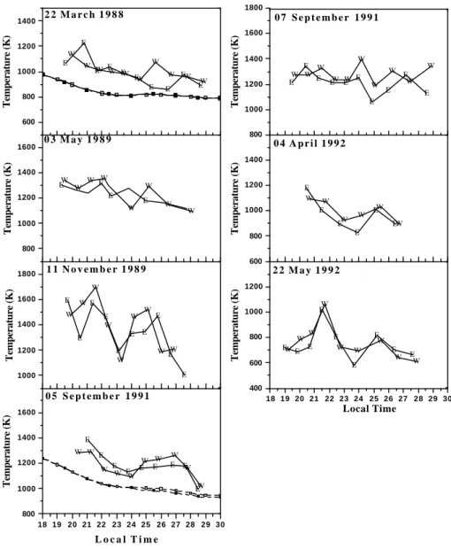
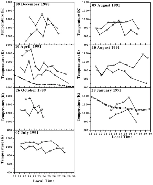
The temperature gradients are more often and prominently observed in the zonal direction at Cachoeira Paulista, but the meridional temperature gradients were also observed on a few occasions. In this paper, we shall concentrate our anal-ysis and discussion only on the zonal direction observations. Figures 2 and 3 show the temperatures observed in the east and west directions for a few representative nights with and
Table 2. Number of nights analyzed with/without thermospheric zonal temperature gradients for three solar flux levels
F10.7[W/m2Hz] < 150 150–200 > 200 Total of Nights
Number of Nights 12 32 29 73 (100%)
With Gradients 4 (33%) 9 (28%) 11 (37%) 24 (33%) Without Gradients 8 (67%) 23 (72%) 18 (63%) 49 (67%)
without temperature gradients. The nighttime temperature variations predicted by the MSIS-90 model (Hedin, 1991) are also presented in Figs. 2 and 3 for some nights and for two different longitudes (23◦S, 41◦W, closed square; and 23◦S, 49◦W, open circle) at the 270 km altitude, but at Ca-choeira Paulista local time. These two locations are close to the positions at which the FPI observes the temperatures in the east and west directions, respectively, from Cachoeira Paulista. Notice that the MSIS-90 model gives, in general, a very small east-west temperature gradient (∼ 25 K over a range of 800 km). Sahai et al. (1992) have reported that the observed thermospheric temperatures at Cachoeira Paulista are in good agreement with the MSIS-86 model for the win-ter and equinox seasons. However, the MSIS model results primarily represent average conditions and do not exhibit the day-to-day variability present in the thermospheric temper-atures. Table 2 shows the details of all the nights analyzed (73 nights) with and without zonal temperature gradients as a function of solar activity.
3.1 Observations without temperature gradients
On most of the nights on which thermospheric temperatures were observed, during the period from 1988 to 1992, the tem-perature to the east and to the west directions at Cachoeira Paulista presented similar nighttime features and magnitude. Figure 2 shows the temperatures observed in the east and west directions for some representative nights without tem-perature gradients. On 49 (67%) out of the 73 nights of observation, the temperature behaviour was similar to that shown in Fig. 2.
It is noted that the observed temperatures in the west and east sectors presented very similar nocturnal variations dur-ing these nights. Also, this behaviour remains the same in both sectors (TE over the sea and TW over the continent) when the observed temperatures presented either smooth nighttime variations (e.g. 22 March 1988) or wave-like varia-tions (e.g. 11 November 1989). On the nights when the ther-mospheric temperature variations showed wave-like struc-tures, it is seen that the temperatures in both sectors pre-sented a similar amplitude of variation (100 K to 400 K). These wave-like variations could possibly be caused by the presence of gravity waves at the thermospheric heights, in periods of a few hours.
-40 -40 -60 -80 0 -10 -20 -30 Cachoeira Paulista Arequipa
Fig. 1. Map of South America showing the location of the
An-des Cordillera (left side - black) and of the Mantiqueira Moun-tains (right side - hatched) and the zonal sub-ionospheric points (∼ 270 km) for Cachoeira Paulista and Arequipa.
3.2 Observations with temperature gradients
During the period studied, 24 nights (33%) showed the pres-ence of significant zonal temperature gradients. Table 2 shows the number of nights that presented zonal tempera-ture gradients and the number of nights that did not, for three different levels of solar activity. It is noted that the oc-currence of zonal temperature gradients is somewhat higher when F10.7 > 200 [W/m2Hz] (37%) than when F10.7is be-tween 150–200 [W/m2Hz] (28%). This indicates that the occurrence of zonal temperature gradients has some depen-dence on solar activity level and this result agrees with that previously presented by Meriwether et al. (1997). However, we find that the occurrence of zonal temperature gradients, when F10.7 < 150 [W/m2Hz] (33%), is similar to that when F10.7 > 200 [W/m2Hz] (37%), but due to the small number of nights (12) when F10.7 < 150 [W/m2Hz], these results must be considered with some reservation. The number of nights analyzed when F10.7is between 150–200 [W/m2Hz] and F10.7> 200 [W/m2Hz] are more significant (32 and 29
1136 P. R. Fagundes et al.: Thermospheric zonal temperature gradients 18 19 20 21 22 23 24 25 26 27 28 29 30 800 1000 1200 1400 1600 1000 1200 1400 1600 1800 800 1000 1200 1400 1600 600 800 1000 1200 1400 18 19 20 21 22 23 24 25 26 27 28 29 30 400 600 800 1000 1200 600 800 1000 1200 1400 800 1000 1200 1400 1600 1800 E E E E E E E E E W W W W W W W W W W E E E E E E E E E E W W W W W W W W W E E E E W W W W W W W W E E E E E E E E E E W W W W W W W W W W E E E E E E E E E W WW W W W W W W E E E E E E W W W W W W E E E E E E E E E E W WW W W W W W W W 0 5 S e p t e m b e r 1 9 9 1 Temperature (K) L o c a l T i m e 1 1 N o v e m b e r 1 9 8 9 Temperature (K) 0 3 M a y 1 9 8 9 Temperature (K) 2 2 M a r c h 1 9 8 8 Temperature (K) 2 2 M a y 1 9 9 2 Local Time Temperature (K) 0 4 A p r i l 1 9 9 2 Temperature (K) 0 7 S e p t e m b e r 1 9 9 1 Temperature (K)
Fig. 2. Nighttime variations of the observed temperatures to the east and west, for representative nights without thermospheric zonal temperature gradi-ents. The temperatures obtained from the MSIS-90 model are also shown for two different longitudes (23◦S, 41◦W, closed square) and (23◦S, 49◦W, open circle) at 270 km of altitude.
nights, respectively), so that these results are more represen-tative. The dependence of the observed temperature gradi-ents on solar activity could be associated with the increase in the F-region electron density with solar activity and pos-sible increase in the transmission of gravity waves from the lower to the upper atmosphere (Meriwether et al., 1997). It should be mentioned that Meriwether et al. (1997) observed thermospheric temperature gradients only during the winter in the high solar activity period, whereas in the present in-vestigations, thermospheric temperature gradients occurred in all seasons with medium to high levels of solar activity. 3.3 Possible mechanisms causing zonal temperature
gradi-ents
Meriwether et al. (1996, 1997) have suggested that the tem-perature gradients observed at Arequipa (16.5◦S, 71.5◦W) are produced by orographic gravity wave viscosity dissipa-tion. They have suggested that low-frequency components of orographic gravity waves are generated at low-altitudes
(tro-posphere) at the Andes Cordillera and propagate vertically to thermospheric heights, where these waves are dissipated, producing a localized region of heating. Also, Meriwether et al. (1997) proposed that the temperature gradients observed at Cachoeira Paulista (23◦S, 45◦W) (Fagundes et al., 1996a) are just a manifestation of the same heating source, since any perturbation in the thermosphere may extend farther to the east, away from the Andes, and then reach Cachoeira Paulista.
Since the thermospheric zonal wind flows eastward dur-ing the night for almost the whole year, neutral air which is heated at Arequipa could reach Cachoeira Paulista. How-ever, this heated neutral air has to travel a distance of approx-imately 26◦(∼ 2600 km) and for a typical eastward wind of 100 m/s at thermospheric heights, this neutral air will reach Cachoeira Paulista about 7 hours later. There is no physical restriction for perturbations travelling from the Andes (Pa-cific) to Brazil (Atlantic), but there are some physical obsta-cles for its occurrence. The typical horizontal distance
be-1 8 be-1 9 2 0 2 be-1 2 2 2 3 2 4 2 5 2 6 2 7 2 8 2 9 3 0 400 600 800 1 0 0 0 1 2 0 0 800 1 0 0 0 1 2 0 0 1 4 0 0 1 6 0 0 1 0 0 0 1 2 0 0 1 4 0 0 1 6 0 0 1 8 0 0 1 0 0 0 1 2 0 0 1 4 0 0 1 6 0 0 1 8 0 0 2 0 0 0 1 8 1 9 2 0 2 1 2 2 2 3 2 4 2 5 2 6 2 7 2 8 2 9 3 0 600 800 1 0 0 0 1 2 0 0 1 4 0 0 400 600 800 1 0 0 0 1 2 0 0 400 600 800 1 0 0 0 1 2 0 0 1 4 0 0 E E E E E E E E E E WW W W WW W W W E E E E E E W W W W W E E E E E E E E E E W W W W W W W W W W E E E E E E W W W W W W W E E E E E W W W W W E E E E E E E E W W W W W W W W W E E E E E E E E W W W W W W W W 07 July 1991 Temperature (K) L o c a l T i m e 26 October 1989 Temperature (K) 10 April 1991 Temperature (K) 08 December 1988 Temperature (K) 28 January 1992 Local Time Temperature (K) 10 August 1991 Temperature (K) 09 August 1991 Temperature (K)
Fig. 3. Nighttime variations of the observed temperatures to the east and west, for representative nights with thermospheric zonal temperature gradi-ents. The temperatures obtained from the MSIS-90 model are also shown for two different longitudes (230◦S, 41◦W, closed square) and (23◦S, 49◦W, open circle) at 270 km of alti-tude
tween the observed east-west sectors in FPI observations is about 800 km. Since we are observing temperature gradients at Cachoeira Paulista of about 100 K to 600 K (Fig. 3), the neutral air flowing eastward has to lose about 12.5 K to 75 K per each 100 km, respectively. Taking into account that the thermospheric neutral air heated at the Andes has to travel
∼ 2600 km to reach Cachoeira Paulista, the total
tempera-ture decrease during this long travel is estimated at 325 K to 1950 K, respectively (considering orographic heating over the Andes as a point heat source). Therefore, it is possible to explain temperature gradients of the order of 100 K at Cachoeira Paulista by taking into account the heating pro-duced at the Andes (Pacific sector). Nevertheless, it is al-most impossible to explain the temperature gradients at Ca-choeira Paulista which are larger than 200 K, without taking into account other sources of localized heating. However, we have to bear in mind that the spatial structure (longitu-dinal/latitudinal) of orographic gravity waves generated over the Andes (which is about 300 km across) is not yet known.
It is, therefore, necessary to consider other possible sources of thermospheric heating in addition to that proposed by Meriwether et al. (1997) for the observations at Cachoeira Paulista. Ionospheric processes, such as ion-neutral cou-pling effects, could provide another source leading to ther-mospheric temperature gradients. However, within the iono-sphere itself, the main longitudinal dependent factor is the geomagnetic field geometry or magnetosphere/ionosphere coupling. Since most of the observations reported here were obtained during relatively quiet geomagnetic conditions and the observation regions are fairly close in space, we could rule out the possibility of longitudinal variations contribut-ing to the observed temperature gradients in ionospheric pro-cesses. Also, as mentioned by Meriwether et al. (1997), mag-netic activity effects would not produce the form of localized heating which is observed.
Hines (1960) drew attention to the importance of at-mospheric gravity waves at ionospheric heights. Sources for medium-scale gravity waves include tropospheric
distur-1138 P. R. Fagundes et al.: Thermospheric zonal temperature gradients
Table 3. Details of tropospheric disturbances in the region of observation on the nights of measurements with/without thermospheric
temperature gradients (Source: Climanalise, a monthly publication by INPE)
# of nights with # of days with meteorological # of days with tropospheric disturbances
observations data available (passage of fronts/or sub tropical jet streams) Nights with E-W
temperatures gradients 24 23 9 (39%)
Nights without E-W
temperatures gradients 49 47 6 (13%)
bances, such as the jet streams, frontal systems and pene-trative convection (e.g. Bertin et al., 1978). Table 3 shows the details of the tropospheric disturbances (fronts and sub-tropical jet streams) present in the region close to the ob-servation site on days with and without thermospheric tem-perature gradients. The Mantiqueira Mountains have sev-eral peaks as high as 2500 m in altitude. Thus, an addi-tional source for some of the observed temperature gradients could be the interaction of the tropospheric disturbances with the Mantiqueira Mountains (which occupies an extensive re-gion around 22◦S, 44◦W), thereby producing large vertical wavelength waves that propagate upward from mountains. Zonal temperature gradients in the thermosphere at low lat-itudes have only been identified in the last 5–10 years and their cause is still not completely understood. More simulta-neous thermospheric and ionospheric observations from re-gions with different topography will be important to pro-vide additional information for a better understanding of the sources of thermospheric zonal temperature gradients at low latitudes.
4 Conclusions
We have analyzed thermospheric temperature variations (on 73 nights) observed at Cachoeira Paulista (23◦S, 45◦W), during the period from 1988 to 1992, under primarily quiet geomagnetic conditions and mid-high solar activity. The main features associated with the occurrence of thermo-spheric zonal temperature gradients are summarized below:
1. Of the 73 nights studied, during the period from 1988 to 1992, 33% of the nights presented thermospheric zonal temperature gradients. Also, the occurrence of zonal temperature gradients have some dependence on the so-lar activity level and are observed in all seasons. 2. One of the possible sources for zonal temperature
gra-dients greater than 100 K (over 800 km horizontal dis-tance), at Cachoeira Paulista, is the heating produced in the Andes by orographic gravity waves, as suggested in a recent study by Meriwether et al. (1996, 1997). Nevertheless, it is not possible to explain the observed temperature gradients at Cachoeira Paulista larger than 200 K, without taking into account other localized heat-ing sources.
3. Orographic gravity waves may be generated at the Mantiqueira Mountains and their dissipation at thermo-spheric heights may induce a localized heating and, con-sequently, produce an additional source for the observed temperature gradients.
Acknowledgements. Thanks are due to Drs. V. B. Rao and P. Satya-murty for helpful discussions related to the tropospheric distur-bances. Partial funding for this work was provided through the Fundac¸˜ao de Amparo `a Pesquisa do Estado de S˜ao Paulo (FAPESP), process N◦95/09297–7 and 97/00810–8, Conselho Nacional de De-senvolvimento Cientfico e Tecnol´ogico (CNPq) No 521243/97–1.
Topical Editor M. Lester thanks P. Dyson and another referee for their help in evaluating this paper.
References
Biondi, M. A., Meriwether, J. W., Fejer, B. G., and Gonzalez, S. A., Seasonal variations in the equatorial thermospheric wind mea-sured at Arequipa, Peru. J. Geophys. Res., 95(A8), 12, 243–250, 1990.
Bertin, F., Kersley, L., Rees, P. R., and Testud, J., Meteorological jet stream as source of medium scale gravity-waves in thermosphere - an experimental study, J. Atmos. Terr. Phys., 40(10), 1161– 1183, 1978.
Bittencourt, J. A., Sahai, Y., Fagundes, P. R., and Takahashi, H., Simultaneous observations of equatorial F-region plasma deple-tions and thermospheric winds, J. Atmos. Terr. Phys., 59, 1049– 1059, 1997.
Fagundes, P. R., Aruliah, A. L., Rees, D., and Bittencourt, J. A., Gravity wave generation and propagation during geomagnetic storms over Kiruna (67.8◦N, 21.4◦E), Ann. Geophysicae, 13, 358–366, 1995a.
Fagundes, P. R., Sahai, Y., Bittencourt, J. A., and Takahashi, H., Observation of thermospheric neutral winds and temperatures at Cachoeira Paulista (23◦S, 45◦W) during a geomagnetic storm, Advances in Space Research, 16(5), 27–30, 1995b.
Fagundes, P. R., Sahai, Y., Bittencourt, J. A., and Takahashi, H., Re-lationship between generation of equatorial F-region plasma bub-bles and thermospheric dynamics, Advances in Space Research, 16(5), 117–120, 1995c.
Fagundes, P. R., Sahai, Y., Bittencourt, J. A., and Takahashi, H., Plasma drifts inferred from thermospheric neutral winds and temperature gradients observed at low latitudes, J. Atmos. Ter. Phys., 58(11), 1219–1228, 1996a.
Fagundes, P. R., Sahai, Y., Takahashi, H., Gobbi, D., and Bitten-court, J. A., Thermospheric and mesospheric temperatures
dur-ing geomagnetic storms at 23◦S, J. Atmos. Ter. Phys., 58 (16), 1963–1972, 1996b.
Fagundes, P. R., Bittencourt, J. A., Sahai, Y., Takahashi, H., and Teixeira, N. R., Plasma drifts inferred from thermospheric neu-tral parameters during geomagnetic storms at 23◦S, J. Atmos. Terr. Phys., 60, 1303–1311, 1998.
Gurubaran, S., Sridharan, R., Suhasini, R., and Jani, K. G., Variabil-ities in the thermospheric temperatures in the region of the crest of the equatorial ionization anomaly – a case study, J. Atmos. Terr. Phys., 57 (6), 695–703, 1995.
Hedin, A. E., Extension of the MSIS Thermospheric Model into the Middle and Lower Atmosphere, J. Geophys. Res., 96, 1159– 1172, 1991.
Hernandez, G. and Roble, R. G., The geomagnetic quiet nighttime thermospheric wind pattern over Fritz Peak observatory during solar cycle minimum and maximum, J. Geophys. Res., 89 (A1), 327–337, 1984.
Hines, C. O., Internal atmospheric gravity waves at ionospheric heights, Can. J. Phys., 38, 1441–1481, 1960.
Meriwether, J. W., Mirick, J. L., Biondi, M. A., Herrero, F. A., and Fesen, C. G., Evidence for orographic wave heating in the equatorial thermosphere at solar maximum, Geophys. Res. Lett., 23 (16), 2177–2180, 1996.
Meriwether, J. W., Biondi, M. A., Herrero, F. A., Fesen, C. G., and Hallenback, D. C., Optical interferometic studies of the nightime equatorial thermosphere: Enhanced temperatures and zonal wind gradients, J. Geophys. Res., 102 (9), 20, 041–058, 1997. Rees, D., Greenaway, A. H., Gordon, R., McWhirter, I., Charleton,
P. J., and ˚Akesteen, The doppler imaging system: Initial obser-vations of auroral thermosphere, Planet. Space Sci., 12 (3), 273– 285, 1984.
Sahai, Y., Takahashi, H., Fagundes, P. R., Clemesha, B. R., Teix-eira, N. R., and Bittencourt, J. A., Observations of thermospheric neutral winds at 23◦S, Planet. Space Sci., 40, 767–773, 1992a. Sahai, Y., Takahashi, H., Teixeira, N. R., Fagundes, P. R.,
Cleme-sha, B. R., and Bittencourt, J. A., Observations of thermospheric temperatures at 23◦S, Planet. Space Sci., 40, 1545–1549, 1992b. Sastri, J. H. and Ranganath, H. N. R., Optical interferometer mea-surements of thermospheric temperature at Kavalur (12.5◦N, 78.5◦E), India. J. Atmos. Terr. Physics, 56 (6), 775–782, 1994. Sipler, D. S., Barry, B. L., and Biondi, M. A., Fabry-Perot
determi-nations of midlatitude F-region neutral winds and temperatures, Planet. Space Sci., 20 (10), 1025–1032, 1982.
Yagi, T. and Dyson, P. L., Measurements of thermospheric tempera-tures at mid-latitude station, Planet. Space Sci., 33 (2), 203–206, 1985.