The effect of carouseling on MEMS IMU performance for gyrocompassing applications

The Effect of Carouseling on MEMS IMU

Performance for Gyrocompassing Applications

by

Benjamin Matthew Renkoski

Submitted to the Department of Aeronautics & Astronautics

in partial fulfillment of the requirements for the degree of

Master of Science in Aeronautics & Astronautics

at the

MASSACHUSETTS INSTITUTE OF TECHNOLOGY

June 2008

@ Massachusetts Institute of Technology 2008

Author ...

. All rights reserved.

..."... .. . .

Department of Aeronautics & Astronautics

// ,< i/ I

May 23, 2008

Certified by...

Certified by...

"'~"'MI'

-Matthew Bottkol

Charles Stark Draper Laboratory

Thesis Supervisor

Emilio Frazzoli

Associate Professor of Aeronautics & Astronautics

Thesis

I,

,

I(\

4

Supervisor

Accepted by ...

JUN 2 4 2009

LIBRARIES

d L. Darmofal

Chair, Committee on Graduate Studies

ARCHIVES

I.

The Effect of Carouseling on MEMS IMU Performance for

Gyrocompassing Applications

by

Benjamin Matthew Renkoski

Submitted to the Department of Aeronautics & Astronautics on May 23, 2008, in partial fulfillment of the

requirements for the degree of

Master of Science in Aeronautics & Astronautics

Abstract

The concept of carouseling an IMU is simulated in order to improve the accuracy of MEMS IMUs. Carouseling consists of slewing the IMU through a pre-determined trajectory that is selected based on inherent properties that lead to improved per-formance. MEMS devices typically have far more uncertainty than standard inertial measurement devices, yet are considerably less massive and require less power, so im-plementing this carouseling scheme could make the use of these lightweight systems possible even in high-accuracy situations, such as gyrocompassing. In gyrocompass-ing, the most significant benefit provided by the carouseling scheme is the reduction in the error contribution of gyroscope bias, as this error is almost completely elimi-nated. Additionally, it was found that although implementing the carouseling scheme required the addition of error states to account for the size effect, in many cases these error states may not be necessary. Overall, the carouseling of the MEMS IMUs was shown to be effective in reducing azimuth error covariance significantly.

Thesis Supervisor: Matthew Bottkol Title: Charles Stark Draper Laboratory

Thesis Supervisor: Emilio Frazzoli

Acknowledgments

First I would like to thank the Charles Stark Draper Laboratory and the Mas-sachusetts Institute of Technology for giving me such an incredible opportunity to broaden my academic horizons. I am profoundly grateful that I had the privilege to attend the most prestigious engineering school in the world and work for one of the most respected labs in aerospace. I would like to thank my thesis advisor Matthew Bottkol for his dedicated support and invaluable guidance during the creation of this thesis. In addition, I would like to thank Olivier de Weck and Emilio Frazzoli, my advisors at M.I.T. who provided me with wisdom and encouragement along the way. Numerous professors and personell at M.I.T., the University of Missouri, and Draper provided me with innumerable amounts of help that assisted me on my journey, and a special thanks goes to the late Michael Ash, who I never had the pleasure to meet, but who did me the great service of bringing me in to the Draper Laboratory.

I thank my parents, Angela and Matthew Renkoski for almost 25 years of unwa-vering support and love. They taught me the benefits of hard work and instilled in me the drive to succeed and do my best in all my endeavors. There is no doubt I never would have accomplished the completion of this thesis if not for their positive and nurturing influence.

A great amount of thanks goes to all my family and friends for the encouragement and kindness they have constantly shown me. I can not imagine a more caring or thoughtful group of people to help me through my thesis or my life. In particular I would like to thank Julie Haesemeier for her unconditional support and dedication. Throughout this thesis writing process she kept my spirits high and was a constant source of inspiration.

This thesis was prepared at The Charles Stark Draper Laboratory under IR&D and Contract GC 009256, sponsored by the United States Army Night Vision and Electronic Sensors Directorate at Ft. Belvoir, VA. Publication of this thesis does not constitute approval by Draper or the sponsoring agency of the findings or conclusions contained herein. It is published for the exchange and stimulation of ideas.

Contents

1 Introduction 9

1.1 Thesis Objective ... ... . 9

1.2 Carouseling Background ... ... 10

1.3 Background on MEMS Instruments . ... 11

2 Carouseling Description 15 2.1 Motivation ... ... .. 15

2.2 The Baseball Stitch Slew ... ... 16

2.3 Analytical basis for Carouseling ... .. 19

2.3.1 Gyroscope Bias Elimination ... 19

2.3.2 Accelerometer Bias Elimination ... 23

2.4 Expanding on the Baseball Stitch Slew ... 25

2.5 Comparing Variations of the Baseball Stitch Slew . ... 28

2.6 Modeling Carouseling ... ... . 42

2.7 Error State Navigation Filter ... ... 44

2.7.1 Covariance and State Propagation . ... 48

2.7.2 Kalman Filter Update ... ... 49

2.8 Size Effect Compensation ... ... 51

3 Gyrocompassing Analysis 57 3.1 Basic description of gyrocompassing ... 57

3.2 Kalman Filter Update ... ... ... 58

3.5.1 Error Budget Formulation . ... ... 70

3.5.2 Sensitivity Analysis Results ... ... 71

3.6 Size Effect Sensitivity ... ... . . 77

4 Conclusions 85 4.1 Carouseling Effect on Azimuth Accuracy .... ... 85

4.2 Size Effect ... ... .. 86

4.3 Other Considerations ... ... 87

4.4 Future Work ... ... ... . . . .. 87

A MEMS IMU Error Specifications 89

Bibliography 89

List of Figures 93

Chapter 1

Introduction

1.1

Thesis Objective

The objective for this thesis is to demonstrate the utility of implementing a carousel-ing technique to improve Inertial Measurement Unit (IMU) navigation performance. The main goal is to see the effect of carouseling in conjunction with Micro-Electro-Mechanical System (MEMS) instruments to see if the improvements in accuracy can lead to the utilization of these instruments in higher-accuracy applications such as gy-rocompassing. This is highly desirable as MEMS instruments are lighter and cheaper than standard IMUs, yet have significantly less accuracy. First the carouseling con-cept will be investigated analytically in order to explore the theoretical benefits asso-ciated with it. Then, to ascertain if carouseling improves performance, the carouseling maneuver will be simulated and navigated with the results compared to those of a standard navigation system.

The remainder of the first chapter of this thesis will provide explanatory back-ground information regarding the carouseling scheme in general and MEMS instru-ments, particularly those developed by Draper. In the second chapter, a more thor-ough investigation of the carouseling maneuver will be undertaken including an in depth analysis of its theoretical benefits. The process for simulating the maneuver and the navigation scheme including the error filter shall be described in detail. The third chapter focuses on the results of the carouseling maneuver when applied to

gy-rocompassing. This includes covariance analysis and sensitivity analysis, including error budget comparisons. Specifically, the error contributions of the size effect in-volved with the addition of lever arm states is investigated. Conclusions and ideas

for future work are included in chapter four.

1.2

Carouseling Background

The concept of carouseling, also known as "slewing" or "maytagging", is a concept that has been developed for use in high-precision scenarios using high accuracy IMUs. The basic operation is to put gimballed IMUs through an inertially referenced slew. The main design of the slewing maneuver is to direct the instruments so that they are pointed in different directions so that the total directional effect is averaged out over time to prevent the build up of biases (the analytical basis and equations of motion regarding this will be examined more thoroughly in Chapter 2). Theoretically the bias errors of both the gyroscopes and accelerometers will vanish at the end of each period since they have not been allowed to build up in any one direction. However, since the IMUs now have an added angular velocity and are not collocated, this could add errors that previously were negligible that could cancel out the improvements made in the biases. Therefore it would be advantageous to fully simulate and investigate the effects of the carouseling maneuver. There is growing interest at Draper and in the navigation community for use of this estimation scheme with current and future MEMS applications. If it is effective in reducing error in MEMS IMUs, it could be a substantial enough improvement so that MEMS devices could be used in place of standard IMUs with little or no loss in quality.

1.3. BACKGROUND ON MEMS INSTRUMENTS

1.3

Background on MEMS Instruments

Micromachined silicon inertial sensors are much smaller and less expensive to produce than standard IMUs. These characteristics make them extremely attractive for real-life systems; especially certain aerospace and military applications where mass is at a premium. MEMS IMUs can be batch produced using semiconductor manufacturing processes which reduces the cost significantly. Additionally, silicon is inexpensive itself and each silicon wafer can contain a large magnitude of inertial measurement devices. The smaller size of the instruments (only a few square millimeters) not only decreases total mass and volume taken up by the instruments, but also leads to reduced power usage; a highly desirable attribute in many applications. All these advantages makes MEMS IMUs an area of much interest, but their lower accuracy has limited widespread use so far.

Draper Laboratory has been developing MEMS sensors for over 15 years, and has become a leader in their development. Draper MEMS instruments have been implemented in various military and space scenarios, including being tested in the use of guiding gun-launched munitions and being designed for use on the Space Shuttle. The MEMS gyroscope Draper has developed a silicon planar tuning fork gyroscope,

photographed by a scanning electron microscope (SEM) in Fig. 1-1.

This model MEMS gyroscope consists of an etched silicon piece anodically bonded to a glass substrate [9]. Like all tuning fork gyroscopes, it contains two vibrating proof masses suspended by beam springs. In this MEMS case, the two symmetrical proof masses are flexurally suspended over capacitor electrodes in the glass substrate. When the device experiences a rotation about its input axis, parallel to the proof mass plane, the Coriolis effect causes the masses to oscillate up and down out of the plane 16].

The amplitude of the resultant motion, which is proportional to the angular rate, is measured by the capacitive plates underneath the proof masses in the glass substrate. This signal is amplified and demodulated by the integrated electronics to provide an output voltage proportional to the angular rate.

Figure 1-1: SEM photo of MEMS tuning fork gyroscope

Draper has also developed MEMS accelerometers which are pendulous mass dis-placement accelerometers 16]. A MEMS 100-g accelerometer is shown in Fig. 1-2.

Figure 1-2: SEM photo of MEMS accelerometer

The accelerometer is also manufactured using a dissolved wafer silicon on insula-tor process that results in an unbalanced proof mass suspended by insula-torsional spring flexures. The proof mass is suspended in a see-saw type configuration so that when there is an acceleration felt by the accelerometer, the proof mass rotates around the

1.3. BACKGROUND ON AMEMS INSTRUMENTS

hinged axis. This motion is measured by capacitive plates in the glass substrate and is proportional to the acceleration, similar to the MEMS gyroscope. This output also provides the input for a closed loop control operation that is used to drive torquer plates to rebalance the proof mass.

These MEMS devices are becoming accurate enough for use in many systems, with improvement continuing. They have been used in guiding projectiles, avionics, and numerous automotive applications. New high aspect ratio etch technology and highly integrated fabrication techniques are increasing the overall performance, theo-retically for use in more high-performance tactical applications in military and space systems. If found to be effective, the carouseling concept could be used to further this performance improvement.

Chapter 2

Carouseling Description

2.1

Motivation

As previously discussed, MEMS instruments provide many desirable attributes for implementation into high-precision applications. However, the desired performance has not yet been achieved in the instruments themselves, so alternative ways to im-prove performance have been developed. One of these concepts is the carouseling scheme which would theoretically improve accuracy and retain the high weight and cost saving associated with MEMS devices. The main goal of implementing an es-timation scheme using carouseling is to eliminate errors due to accelerometer and gyroscope biases. As described earlier, the basic theory is that if the IMU was spun around in a certain trajectory which will average out the pointing of the IMU so that no direction is favored, the build-up of gyroscope biases would be eliminated. If this process can improve accuracy enough, MEMS devices could then be implemented in higher accuracy applications. There would be additional mass associated with the slewing device, but this could be minimized so that the total system would still be significantly smaller and require less power than a conventional IMU.

This chapter will investigate the analytical basis for the performance improvement and describe the kinematics of the carouseling scheme. First the slewing maneuver

itself will be introduced and its effect on the contributions from gyroscope and

ac-celerometer error shall be analyzed and simulated. Variations of the original slew will

be developed and compared to select the optimum slewing motion to eliminate the

most error. Then the equations used to simulate the slewing maneuver with error

contributions will be developed as well as navigation equations, including filter

up-dates. Finally, the complications of the addition of lever arms and the size effect will

be investigated more fully.

2.2

The Baseball Stitch Slew

Carouseling is meant to reduce gyroscope and accelerometer biases by averaging each

axis to be pointing in all directions for an equal amount of time. The concept is that

since biases are directional errors that build up along an axis, if the overall direction

is averaged out by the slewing trajectory, the net effect of the bias errors will go to

zero. If the IMU can then be made to follow a trajectory that properly averages out

this effect, then the bias contribution to the total error would vanish at the end of

each period. Therefore, the first task is to select a trajectory that accomplishes the

desired effect.

There are a number of slews that achieve this characteristic, the most common

being what is called the Baseball Stitch Slew, so named for its resemblance to the

path of the stitching along a baseball. The baseball stitch slewing maneuver can be

mathematically described as the combination of two orthogonal rotations with the

angular velocities of the two rotations related by an integer ratio. For example, in the

commonly used 2:1 baseball stitch slew, the second gimbal rotation has double the

angular velocity of the first. To create this motion, each IMU will be dual-gimballed

so it is allowed to follow the specified path controlled by servo-mechanisms operating

each rotation. This rotation is performed in the inertial reference franme, which is an

important property of the baseball stitch slew. The slew is essentially a rotation from

2.2. THE BASEBALL STITCH SLEW

body coordinates to inertial coordinates. Figure 2-1 shows the baseball stitch slew in a three dimensional representation, demonstrating the trace of the endpoint of one axis for the duration of the slew. Now that the concept of the baseball stitch slew is

... .. . ... .]. ..

S

i

...

..

...

.

...

...

...

i

_.

_.

_...

Figure 2-1: 3-D Trace of a 2:1 Baseball Stitch Slew Depiction of the three dimensional trace of the endpoint of one of the rotating axes, closely resembling the stitching of a baseball

established, its properties of importance can be analyzed. The equations governing its motion will be produced and summarized in this section to provide the basis for this analysis. In matrix form, the 2:1 baseball stitch rotation, Rbs, can be represented as the combination of the two orthogonal rotations comprising the slew:

sin(wt)

0

cos(wt) cos(2wt)

cos(wt)

where w is the angular velocity of the first rotation matrix and t is time. In this case, it can be seen the first rotation is about the z-axis and the second rotations is at twice the angular rate and performed about the x-axis. It is important to remember this slew is inertially referenced, not Earth-fixed. The baseball stitch slew Rbs(t), has a valuable property which will be addressed later in this section that demonstrates the benefit of its implementation.

To find the angular velocity, use the following equation to define the time rate of change of any three-axis rotation:

R

= R[ x]

(2.2)

where [ x] is the skew symmetric form of the angular velocity vector, = (w, W2, W3). The skew symmetric matrix representation of the angular velocity takes this form:

0 -w3 L2

[Ux] = W)3 0 -L)1 (2.3)

--W)2 L1 0

Again, this rotation R is the transformation from the body axis to the inertial axis and the angular rates are in the inertial frame. This is important as gyroscopes measure inertial rates, since they are inertial instruments. Using the rotation Rbs(t) from Eq. 2.1 as the rotation matrix in Eq. 2.2, the vector 0 can be solved for to yield

2w

Qbs = csin(2ct) . (2.4)

w cos(2wt)

This angular rate vector Obs is the output of an ideal gyroscope which is fixed to a body that executes the baseball stitch slew with respect to inertial space.

2.3. ANALYTICAL BASIS FOR CAROUSELING

2.3

Analytical basis for Carouseling

In this section the knowledge gained from Section 2.2 will be used to show how gyroscope and accelerometer biases can be eliminated using the baseball stitch slew. Basic equations of motion will be introduced that will be implemented later into the navigation scheme, but the main focus of this section will be solely on the effect of the baseball stitch on these equations. The overall navigation scheme will be fully described in Section 2.7.

2.3.1

Gyroscope Bias Elimination

In order to better understand the effect of slewing on gyroscope bias error, it is important to see what makes up the gyroscope error contribution to angular velocity, defined here as 6Q.

To find this error, first linearize Eq. 2.2, where R(t) is the body to inertial coordinate transformation, to result in

b = 6R[ x] + R[6 x] (2.5)

where the gyroscope error 6Q is the error in sensed angular rate. It can be assumed that the error in the angular rotation can be represented as an error rotation matrix in body coordinates, called T. This can be defined by Eq.2.6:

6R = R[ix]

(2.6)

This can be substituted into Eq. 2.5 to yield

which can be be converted into a vector equation in body coordinates as

I = -Q

q + mO.

(2.8)

To express the error in inertial coordinates, differentiate the equation

I = R(t)F _(2.9)

where I' is the error rotation in inertial coordinates. After differentiating Eq. 2.9 and substituting the result of Eq. 2.8, this results in

d

MI

= RW+

4R

dt

= R(-Q x x, + 6Q) + R[ x]q,

Therefore the total contribution from the gyroscope error to the error rotation in the inertial frame is simply the gyroscope error multiplied by the rotation matrix. Now the gyroscope error 6Q, can be broken down into its components to further examine the contribution to the error. The gyroscope error can be assumed to be consisting of four main error sources: gyroscope bias error bg, gyroscope scale factor sfg, gyroscope misalignment m,, and gyroscope non-orthogonality ng. Each of these quantities are vectors consisting of 3 scalar values (one in each direction of the body frame). The errors are inherent to the gyroscope itself and are a function of the error characteristics of that gyroscope. They can be combined to form the overall gyroscope error in the following equation:

2.3. ANALYTICAL BASIS FOR CAROUSELING

where [sfg,] represents a 3 x 3 diagonal matrix formed from the 3-vector containing the gyroscope scale factor errors, sfg = (sfl, sf2, sf3), in the following way:

sfi 0 [sfg] = 0 s f2 0 0

0

s

f3

0

-m2

formed from the three misalignment error

-m3 0 M1 (2.13) m2 -m ₁ 0

and [ng®] is a symmetric 3x3 matrix created from the non-orthogonality terms of

the 3-vector n, = (ni, n2, n3), such that

0 [ng®] = n3 n2 7i n2

1

Now that these matrices have been defined, the can be calculated by integrating Eq. 2.10 from and combining it with Eq. 2.11:

change in the rotation error, AI', time zero to some discrete time T,

A I -

j

I/

= TR(t)

(b

Equation 2.15 can be rewritten by distributing the diagonal, skew-symmetric, and symmetric matrix representations to the angular velocity vector Q, instead of the

scale factor, misalignment, and non-orthogonality error vectors, respectively. The results of this re-distribution create Eq. 2.16:

,A* =

()

+

[.]sfg

-

[l

x]m

+

[

]ng)

(2.16)

This puts the equation into a form that can be more easily used to demonstrate the effect the slewing motion has on the rotation error. Notice that the diagonal and symmetric operations can switch to apply to the vector 0 and cause no change, while changing the skew-symmetric operation from the misalignment vector to Q results in a change in sign.

Now the gyroscope error source vectors can be completely separated from the integral, since they are assumed to be constant, and Eq. 2.16 can be rewritten as

Ak I = SB(T)bg + SSF(T)sfg + SA,(T)mg + SN(T)ng (2.17)

where the matrices of the form Sx are known as "sensitivity matrices" and are integrals used to quantify the effect of the four error sources on the rotation error matrix. The sensitives are all integrals over the time interval 0 - T that result in 3 x 3 matrices.

The bias, scale factor, misalignment, and non-orthogonality sensitivity matrices can be respectively described as:

SB(T) = T (2.18)

S(,(T) =

[0(

)(t)dt,

(2.19)

/T

SA,(T) = - R(t) [Q(t) x]dt, (2.20)

S (T) J R(t) [ (t)(] (t)dt. (2.21) The baseball stitch slew, with rotation matrix

Rb,

particu-2.3. ANALYTICAL BASIS FOR CAROUSELING

larly interesting and useful because it has the property,

SB(T)

=

Rbs (t)dt = 0.

(2.22)

This mathematically expresses the fact that the overall accumulation of the rotation

Rbs is zero, meaning over time T no one direction is favored. To prove this, it can be

seen that integral of each element in the baseball stitch rotation matrix from Eq. 2.1 equals zero when taken over the time of one period. The integral of the trigonometric functions sin and cosine over one period is always equal to zero and using the property of orthogonality of the trigonometric functions, the integral of the other elements of the rotation matrix will also be equal to zero. Since this entire integral is zero, the sensitivity matrix in Eq. 2.18 is equal to zero, and it eliminates the contribution of gyroscope bias to the overall rotation error A*, in Eq. 2.15. Since the bias sensitivity matrix goes to zero, no matter how large the gyroscope bias error, its contribution will always vanish at time T when the baseball stitch slew is performed. In this way the baseball stitch slew is shown to achieve the goal of eliminating the contribution from the gyroscope bias error, but no other error source. The elimination of these other gyroscope errors will be investigated in Section 2.4.

2.3.2

Accelerometer Bias Elimination

While the previous subsection detailed how gyroscope bias errors can be eliminated by carouseling using the baseball stitch slew, contributions from accelerometer bias to the error in acceleration can also be reduced. In fact, it was for the express purpose of eliminating accelerometer bias error that the slew was developed, and was later found to also eliminate the gyroscope bias. However, in the gyrocompassing application, the attitude error is more important than the velocity error so the gyroscope errors are more crucial.

rotation error. However, accelerometer error plays a large part in the error in velocity felt by the IMU. In the following equation, derived from equations of motion, can be seen the components of error in acceleration:

= G(t)6x - 2[QE x]5v + R[ ×x]f +

6a

where 6a is the accelerometer error. The derivation of this equation and the components of the first three terms will be described in detail in Section 2.7, but for now the only term of concern is the accelerometer error. It can be assumed that the accelerometer error is made up of the contributions from four sources, much like the gyroscope error: accelerometer bias, scale factor, misalignment, and nonorthogonality. They combine to contribute to the total accelerometer error as follows:

aa = R(6ba + [f-]6sfa - [fx]6ma + [f0fn) (2.24)

Where R is the body to inertial coordinate rotation used in the gyroscope equa-tions as well. Ignoring the first three terms and integrating Eq. 2.23 with Eq. 2.24 inserted for Sa, the contribution of accelerometer error to the velocity error can be

seen:

T v =

6adt

/T0

v = SB(T)ba + / R([f.]sf -

Lfxlma

where SB(T) is the bias sensitivity matrix from Eq. 2.18 in the previous section, and has been proven to vanish over the time interval 0 - T when using the baseball

stitch slew. Therefore, the contribution from accelerometer bias error to the velocity error vanishes as well, no matter what the accelerometer bias value is. Even though the area of research for this thesis is the gyrocompassing application, which is far

2.4. EXPANDING ON THE BASEBALL STITCH SLEW

25

more concerned with the angle error, this increased performance in the velocity error is still a valuable attribute of the carouseling scheme. And although this does not directly increase accuracy of the azimuth angle, when filtering is used and all errors are intermixed, better accuracy in any measurement can contribute to overall accuracy.

2.4 Expanding on the Baseball Stitch Slew

As was shown in Section 2.3, the baseball stitch slew is effective in eliminating the contribution of gyroscope bias to the total error rotation I. However, it does not eliminate contribution from other error sources, namely the integrals SsF(T), SM,(T), and SN(T) do not reduce to zero at the end of each period. So while the bias term returns to zero, these other errors continue to accumulate. This is undesirable, but it has been found that by modifying the baseball stitch slew, these errors can also be eliminated. In this section, modifications to the baseball stitch slew will be made that will make it more effective at improving accuracy. In order to provide a goal for the improved slew, the sensitivity matrix format will again be used to determine another possible way for carouseling to provide benefits. To investigate this problem, first create the matrix expression

M = [sfg,] + [m,x] + [n₉®] (2.26)

which can be seen in Eq. 2.11 as the 3 x 3 matrix multiplied by the angular velocity to contribute to the gyroscope error. Also notice that this matrix M is given by nine free parameters, so it can be said to represent an arbitrary 3 x 3 matrix with nine free entries. From this knowledge it can be proven that the three sensitivity matrices it is desired to eliminate (SsF(T),SnA(T), and SN(T)), will be equal to zero if and only if

-R(t)MA(t)dt

for any 3 x 3 matrix Al. That is, no matter the magnitude of

Al

R(t) must be found that satisfies Eq. 2.27. This equation holds true no matter the

value of M, which means no matter how poor the accuracy, with the right rotation, the error contribution for all three of these sources can be eliminated at time T.

Now a slew will be created that satisfies the above equation while still satisfying Eq. 2.22 as well. The equations governing this slew will be developed and then it will be proven that it does satisfy equation 2.27. This new slew can be created from the concept of reversing the baseball stitch slew. The IMU will travel through the slew completely, and then travel over the same trajectory in the opposite direction. This was created to "unwind" the effects of scale factor, misalignment, and nonorthogo-nality, while still eliminating the bias contribution. To investigate the effects of slew reversal, define slew R+(t) to be any slew, and create a piecewise slew R(t) defined as

R(t)

R±(t)

O<t<T

(2.28)

R(t) T<t<2T

where R_(t) is the reverse in time of R+(t) and can be mathematically defined as:

R_(t) = R(2T - t)

T < t < 2T

(2.29)

From Eq. 2.2, the time rate of change for the rotations can be defined as

R+ (t) = R+(t)[Q(t)x] 0 t < T (2.30)

R_(t) = R (t)[_ (t)x] T < t < 2T (2.31)

2.4. EXPANDING ON THE BASEBALL STITCH SLEW

to obtain

R_(t) = -R±(2T-t)

= -R+(2T-

t)[,+(2T - t)x]

(2.32)

Setting Eq. 2.32 equal to Eq. 2.31 and using Eq. 2.29 produces

I_

(t)

R_(t)[_ (t)x]

-R+(2T-

t)[Q+(2T-t)x]

[Q_(t)x] = -[a+(2T-t)x]

-(t)

= 2+(2T- t) (2.33)

over the interval T < t < 2T. Using this relation, it can be shown that Eq. 2.27 is

true for any trajectory that undergoes a slew reversal as described in Eq. 2.28. Take Eq. 2.27 and use the definitions of the rotation matrix and angular velocity with slew reversal to show 2T R(t)M (t)dt

R+(t)M +(t)dt

R(t)M

R+(t)MQ+(t)dt

R+(2T

t)MA+(2T

+(t)dt +

R+(t)()MOa(t)dt

Notice that this is true for any 3x3 matrix M and by Eq. 2.27, SF(2T),SI(2T), and

SN(2T) will all be equal to zero when there is a slew reversal. Notice also that this

holds for any rotation R(t), not necessarily the baseball stitch slew. However, since it is based on the baseball stitch slew, Eq. 2.22 still holds true and the contribution due to both accelerometer and gyroscope biases will continue to vanish at the end of

each period. Combined with the reversal, the contribution of all four gyroscope error sources is now seen to vanish.

2.5

Comparing Variations of the Baseball Stitch Slew

To better compare the effects of the baseball stitch slew and its derivatives in terms of their contribution to T, this section will focus on exploring the error contributions in Eq. 2.17 graphically for each slew.

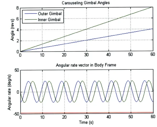
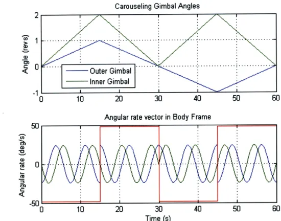
For the regular baseball stitch slew, first observe the motion of the gimbal angles over a period of 60 seconds (implementing Eqs. 2.1 and 2.4).

Carouseling Gimbal Angles

~%

'4 <2

0

10 20 30 40 50

Angular rate vector in Body Frame

-50 1

0 10 20 30 40 50

Time (s)

Figure 2-2: Plots Slew

of gimbal angles and angular rates of a 60 second Baseball Stitch

2.5. COMPARING VARIATIONS OF THE BASEBALL STITCH SLEW

29

as the slew progresses an the gimbals continue to rotate constantly in one direction, with the outer gimbal increasing at twice the rate as its rotation has twice the angular velocity. The second subplot shows the angular velocity components for the entire slew. Notice two of the angular velocity components follow sinusoidal behavior while the third element remains a constant equal to the angular rate of the second slew, as was shown in Eq. 2.4.

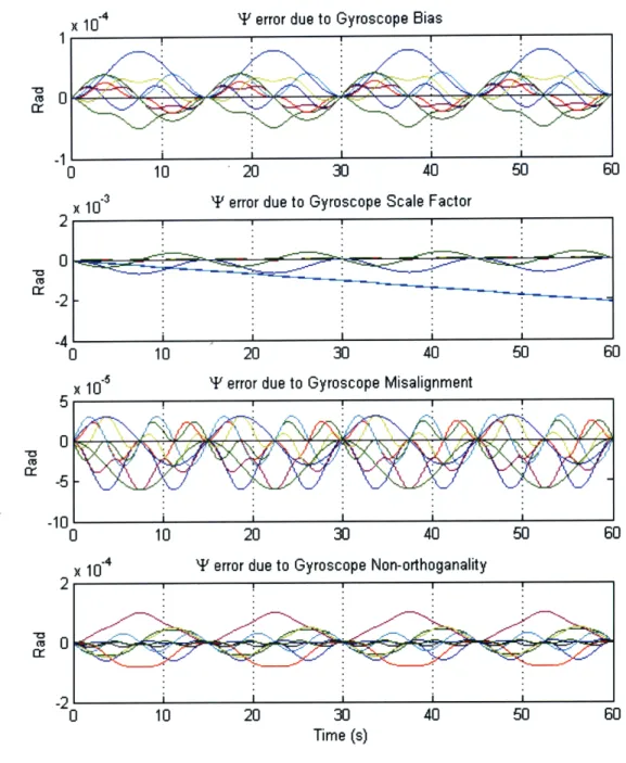
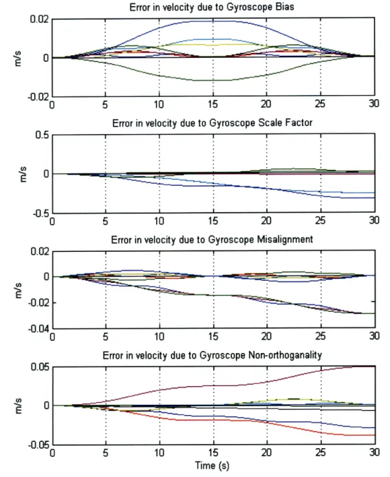
Now performing the integrations of the sensitivity matrices in Eq. 2.17, the total contribution to the rotation error can be plotted for the baseball stitch slew. Values for the gyroscope bias, scale factor, misalignment, and nonorthogonality errors are assumed to be those of the current Draper MEMS IMU model, which will be discussed later in Section 3.3 (the specifications can be found in Table A.1 in Appendix A). The exact values of the errors are not important at this point, but rather the pattern of behavior of the error contributions over time for one period. In Fig. 2-3 is plotted the contributions of each error term to the 9 elements of the AI matrix in Eq. 2.17 for the baseball stitch slew.

Notice the bias terms vanish at the end of the period as was shown from Eq. 2.22. Also the misalignment and non-orthogonality contributions do vanish, but two ele-ments of the scale factor error continue to build up. Note that the bias, misalignment, and non-orthogonality errors not only vanish at the end of the period, but also every 15 seconds which is equal to one fourth of a period. As can be seen in Fig. 2-2, this corresponds to the times when both gimbals have performed a whole number amount of revolutions. Also observe that the scale for the plot of the error contribution due to gyroscope scale factor is an order of magnitude larger than the scale use for the other three error sources. These errors combine to form the total rotation error shown here in Fig. 2-4.

In Fig. 2-4 it can be seen that most of the error elements return to zero at the end of each period, but two elements attributable to the scale factor error still continue to build up. The errors that do return to zero oscillate in the manner observed before

T error due to Gyroscope Bias

10 .20 30 40 50

T' error due to Gyroscope Scale Factor

!I I | I

0

-2

-41

0 10 20 30 40 50 E

Y error due to Gyroscope Misalignment

10 20 30 40 50

'1 error due to Gyroscope Non-orthoganality

-EJ

-21

0 10 20 30 40 50 60

Time (s)

Figure 2-3: Contributions of different error sources to the overall rotation error for the Baseball Stitch Slew

x 10.4 x 10.3 x 10"5 5 0 -5 -10 x 10.4

2.5. COMPARING VARIATIONS OF THE BASEBALL STITCH SLEW

x 103 Total Error in y

0.5 1 1 ,

10 20 30 40 50

Time (s)

Figure 2-4: The total contribution Baseball Stitch Slew

to rotation error from gyroscope errors for the

in which they also return to zero ever one fourth of a period. As a point of reference, compare the above plot to the total error for a non-rotating MEMS IMU (i.e. the rotation matrix is equal to identity in Eq. 2.17), which yields the total error plot seen in Fig. 2-5.

First, notice that only one element changes from zero, and that is known to be due to the bias. The other errors contribute no error as the body is not moving. So even though the baseball stitch slew does an excellent job of eliminating the gyroscope bias, by introducing rotation, the other errors become a factor. And even though misalignment and non-orthogonality are also cyclically eliminated, the scale factor error builds up which effectively eliminates the improvements made in reducing the bias. In fact, Fig. 2-4 shows that the additional scale factor error grows slightly

0

-0.5

-1.5

-2

Total Error in T

10 20 30 40 50

Time (s) Figure 2-5: The

rotating body

total contribution to rotation error from gyroscope errors for a

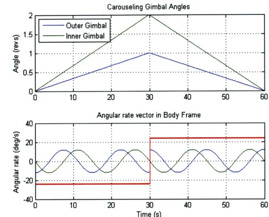
non-larger than the original bias error seen in Fig. 2-5. So the normal baseball stitch slew performs well at eliminating bias, misalignment and nonorthogonality, but the addition of the scale factor makes it unattractive for implementation. However, as discussed in Section 2.4, if the baseball stitch slew performs a reversal as defined in Eq. 2.28, the scale factor error will also reduce to zero at the end of each period. For the baseball stitch slew with reversal, the gimbal angles and angular velocity now behave as seen in Fig. 2-6.

As can be seen in the figure, both gimbals are reversed halfway through the 60 second slew. Instead of the gimbal angles continuing to increase, they now reverse direction and are in fact both equal to zero at the end of the period. Notice the

x 10.3 1 0.9 0.8 0.7 0.6 " 0.5 0.4 0.3 0.2 0.1

2.5. COMPARING VARIATIONS OF THE BASEBALL STITCH SLEW

Carouseling Gimbal Angles

40 20 cc 0 -20 -40 0

Angular rate vector in Body Frame

10 20 30 40 50 E

Time (s)

Figure 2-6: Plots of gimbal angles and angular velocities for Baseball Stitch Slew with

Reversal

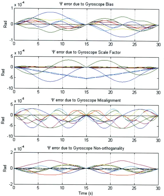
elements of angular velocity reverse sign at the time of slew reversal as well. Once again using Eq. 2.17, but this time integrating the baseball stitch slew with reversal rotation, the contributions to the 9 elements of the A'I matrix can be seen for the baseball stitch slew with reversal in Fig. 2-7.

Now all nine elements of the four error source sensitivity matrices return to zero at the end of the slew. This is the exact result desired. It would appear that the baseball stitch slew with reversal would be the best slew to use for carouseling, but there is another aspect that has not been taken into account.

Although the focus of gyrocompassing is on the azimuth angle so the velocity error is not the main concern, in the real navigator using a Kalman filter, it is still highly desired to have accurate velocity measurements. So to better ascertain if the

--- Outer Gimbal I-nner Gimbal .. . .. . . .. . .. .. . . .. . . . .. . . . .. . . .. . . . ° ° -. ... .... ... .... .. ... ... .... . ... ... . ... . ... ... .. ... .. ... ...... .. ..' I ! | |

T error due to Gyroscope Bias

3 5 10 15 20 25 30

x 104 _{T error due to Gyroscope Scale Factor}

y error due to Gyroscope Misalignment

5 10 15 20 25 30

'1 error due to Gyroscope Non-orthoganality

0 5 10 15 2

n

Time (s)

Figure 2-7: Contributions of different error sources to the overall rotation error for the Baseball Stitch Slew with Reversal

x 10-4 10 -0 x 10, x x 10,4 -10 2 0 -2

2.5. COMPARING VARIATIONS OF THE BASEBALL STITCH SLEW

35

baseball stitch with reversal is the optimum slew, it would be valuable to investigate the gyroscope error contribution to the velocity error as well.

Recall from Eq. 2.23, that the I error actually does contribute to the velocity error in the third term, which is R['IFx]f. If the result for AkF from Eq. 2.17 is inserted for * , this can be integrated to determine the contribution of the gyroscope errors to the velocity error (represented as Av in this analysis):

Av(T) = Aq x f(t)dt

= jT(SB(T)b + SsF(T)sf + SM(T) mg + S(T)ng) x f(t)dt(2.35)

In this equation _{it can be seen that instead of the error contributions merely} being the sensitivity matrices, it is now the integral of the sensitivity matrices that determines the contribution to the velocity error. Performing the integrations in Eq. 2.35 for the baseball stitch slew with reversal yields the results shown in Fig. 2-8.

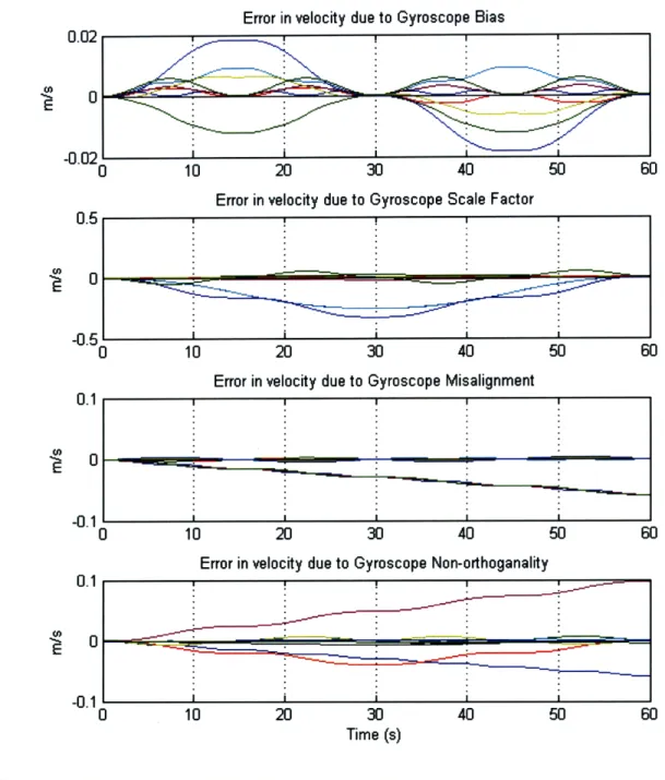
Notice the contribution due to gyroscope bias continues to vanish, however the other three sources continue to build up. Particularly the error contribution due to scale factor is a problem, as it is an order of magnitude greater than the misalignment and non-orthogonality errors. So the slew reversal fails to eliminate these errors. However, it has previously been found that this reversal concept can be extended to provide better performance. As there are two separate gimbals, both gimbals do not have to be reversed simultaneously. It was discovered that a concept involving only reversing the outer gimbal every other time would improve upon the performance of the baseball stitch slew with reversal. The plots of the gimbal angles and angular velocities for this scheme, called the baseball stitch slew with reversal extended can be seen in Fig. 2-9.

This figure demonstrates how the outer gimbal is not reversed at 30 seconds when the inner gimbal is reversed. Also notice that when the next period starts the inner

Error in velocity due to Gyroscope Bias

-" " ' '--- --- ".. _ . . : _ _--- -

-Error in velocity due to Gyroscope Scale Factor

0 5 10 15 20 25 31

Error in velocity due to Gyroscope Misalignment

3 5 10 15 20 25 30

Error in velocity due to Gyroscope Non-orthoganality

I •

I I

Time (s)

Figure 2-8: Contributions of different gyroscope error sources to the change in velocity error for the Baseball Stitch Slew with Reversal

0.02 0 -0.02 0 -0.5 0.02 0 -0.02 -0.04 0.05 0 -0.05

I

I

2.5. COMPARING VARIATIONS OF THE BASEBALL STITCH SLEW

Carouseling Gimbal Angles

- Outer Gimbal - Inner Gimbal

D 10 20 30 40 50 61

Angular rate vector in Body Frame

i t~I I t lt iVI' I~

-50

0 30

Time (s)

Figure 2-9: Plots of gimbal angles and angular velocities for Baseball Stitch Slew with

Reversal Extended

gimbal will be reversed but the outer gimbal continues to rotate in the same direction. To verify that this slew continues to provide the nulling capabilities of gyroscope error contribution to A* of the baseball stitch with slew reversal, Eq. 2.17 can again be used to plot out these results for the baseball stitch with slew reversal extended, shown here in Fig. 2-10.

Notice that all the error contributions continue to vanish at the end of each period, and also the scale factor contribution vanishes at the 30 second mark. The other three sources show the familiar behavior of all elements returning to zero at each one fourth of a period. It is interesting to note that the error contribution plots for each source can be divided at the 30 second point and the two halves are reverse images of each other.

Y error due to Gyroscope Bias

I

I I i I

0 10 20 30 40

x 103 _{T error due to Gyroscope Scale Factor}

10 20 30 40 50

T error due to Gyroscope Misalignment

10 20 30 40 50

T error due to Gyroscope Non-orthoganality

10 20 30 40 50 E

Time (s)

Figure 2-10: Contributions of different error sources to overall rotation error for Base-ball Stitch with Reversal Extended

x 10-5 x 10.4 2 (0 tr -20 SI I I SI i I x 10-4 1,I~ 3

2.5. COMPARING VARIATIONS OF THE BASEBALL STITCH SLEW

39

Now to investigate if the baseball stitch with reversal extended provides any benefit in the velocity error, the error contributions to the velocity error are presented in Fig. 2-11.

The scale factor error contribution is now reduced back to zero at the end of the period, along with the contribution from the gyroscope bias. Unfortunately, the misalignment and non-orthogonality errors persist, but their error contribution is significantly less than the previous contribution from scale factor for the simple reversal in Fig. 2-8. These misalignment and non-orthogonality errors are therefore not of critical importance to eliminate, and as will be seen in the simulations, their contributions are minimal and do not greatly impact azimuth error.

The total error contribution from gyroscope errors to F for the baseball stitch slew with reversal extended can be seen in Fig. 2-12:

Now the contributions from all error sources vanish at the end of the period. The scale factor error does not build up like it did for the normal baseball slew as seen in Fig. 2-4, and the bias terms do not continue to grow as seen when no rotation at all is applied as seen in Fig. 2-5. All errors reduce back to zero and do not grow larger than 8 x 10- 4 radians in magnitude at any point, with most elements remaining significantly smaller than that, including all reducing to zero at the mid-point as well. It is important to note that all of these results are for ideal cases where there is no filtering and no updates whatsoever. In real applications there will be filter updates that will affect the contributions of these error sources. Cross-correlations will develop and other error sources such as random walk are incorporated into the navigation as well. Therefore, the exact results found in this section should not be expected to be repeated in the simulations. However, the belief is that the trends seen here will be reflected in the results, as in, it is expected to see that the carouseling will reduce the effects of gyroscope error sources on angle error. It is not expected that these contributions will be exactly zero or that any of the other errors will show identical behavior to what has been demonstrated in these idealized plots.

Error in velocity due to Gyroscope Bias

10 20 30 40 50

Error in velocity due to Gyroscope Scale Factor 0.02 0 -0.02 0.5 0 -0.5 0.1 0 -0.1 0.1 0 -0.1 C Time (s)

Figure 2-11: Contributions of different gyroscope error sources to velocity error for Baseball Stitch with Reversal Extended

Hi

i

Error in velocity due to Gyroscope Non-orthoganality

i --L l ~---L --I -I I I ---~ I i i 1 I

Error in velocity due to Gyroscope Misalignment

-2.5. COMPARING VARIATIONS OF THE BASEBALL STITCH SLEW

x 10-4 Total Error in Y

0 10 20 30 40 50 60

Time (s)

Figure 2-12: Total Contribution to angle error from gyroscope errors for Baseball Stitch Slew with Reversal Extended

Now that the baseball stitch slew with reversal extended as been shown to be superior to the regular regular baseball stitch slew, it will be selected for use in the navigation simulations. There would be no practical reason to implement the regular baseball stitch slew instead of the slew with reversal extended as it performs either the same of better in all areas. As the term "baseball stitch slew with reversal extended" is a long and convoluted phrase, for the remainder of this thesis, the slew will be referred to simply as the "baseball stitch slew", unless otherwise specified. So when the baseball stitch slew's performance is referred to from now on, it is understood to be referring to the baseball stitch slew with reversal extended.

2.6

Modeling Carouseling

The theoretical benefits of carouseling have been shown, but the real goal of this thesis is to show what these benefits equate to in a numerical simulation which models the true performance of MEMS IMUs in real-life applications. The first step is to simulate the output of the IMU experiencing the slew with ideal accelerometers and gyroscopes at the center of the rotation. In reality, the IMUs will most likely not be collocated at the center of rotation and this has potentially serious implications, called the size effect, which will be investigated in Section 2.8. This section will be concerned with establishing the equations used to model the baseball stitch slew and generate the IMU outputs angular velocity and specific force. First the ideal outputs will be created (i.e. no accelerometer or gyroscope errors added), then the errors will be incorporated to create a simulated IMU output.

The ideal gyroscope output is the angular velocity vector Q, which has been defined for the baseball stitch slew in Eq. 2.4 and for the reversal in Eq. 2.33. The output of an ideal accelerometer is the specific force f felt by the accelerometer in the body frame. This includes the acceleration of the navigation point in the body frame and the gravitational acceleration:

f = R' - GB (2.36)

where RB is the rotation from the Earth Centered Inertial (ECI or simply, inertial) frame to body coordinates. In this case RB is the inverse of the baseball stitch slew, Rb8 = R . The acceleration of the navigation point, x' in inertial space is defined

as 3', which is determined by the trajectory of the overall body, i.e. if the navigated point is standing still on the earth, the only movement will be due to the rotation of the earth (and there will be no movement observed when using local level coor-dinates). If the IMU is being used for missile guidance, the missile's trajectory and flight path will determine the motion felt by the body. The determination of the

spe-2.6. MODELING CAROUSELING

cific trajectory must also be modeled and will be discussed when applying to specific situations. Also note that superscripts on variables indicate the coordinate frame of reference, and for rotations, the subscript indicates the initial frame and the super-script indicates the frame into which the rotation is being performed.

The gravitational acceleration contains both the effects of gravity and the cen-tripetal acceleration induced by the Earth's rotation:

GB = (g(x) - [QearthX]2XI)RB (2.37)

where g(x') is the expression of gravitation depending on the inertial location of the navigation point. This can be approximated by linearizing and ignoring perturbation effects as:

g(x) =X (I - 3uuT) (2.38)

where p is the universal gravitational constant and u is the unit vector in the direction of xI. The quantity [Kearth X ] is the skew symmetric formed from the earth's rotation vector defined as

0

Qearth = 0 (2.39)

[Wearth

where Wearth is equal to the angular velocity of the Earth's rotation. As was stated earlier, the specific force and angular velocity are the outputs of ideal inertial mea-surements, meaning there are no measurement errors. In application, there are ac-celerometer and gyroscope errors in the measurements. Therefore, these errors must be simulated as well and their contributions taken into account. The simulated out-puts, designated as a for accelerometer output and g for the gyroscope output vector

are simulated as:

a = f + R(ba + [f-]sfa - [fx]ma + [f @]na) + Wa (2.40)

g = + b + [Qg.]sf - [x]m, + [W ]ng + wg (2.41)

where the subscript a signifies an accelerometer error source and the subscript g signifies gyroscope errors. The bias and scale factor terms are simulated as Markov processes as well as constants and the misalignment and non-orthogonality terms as random variables with covariances determined by the specific IMU. In addition to the instrument errors, random walk effects, w, also affect both the accelerometer and gyroscope output. The random walk can also be simulated as a random process with specified covariances. Using Eqs. 2.40 and 2.41, the output of an IMU undergoing carouseling can be simulated. An estimation scheme must be developed to navigate this data so the performance can be evaluated.

2.7

Error State Navigation Filter

In order to navigate the slew (or any standard strap down system) an integration scheme must be developed. In this section the basic concept of the navigator will be described and the equations of motion will be presented and linearized. Subsection 2.7.1 presents the covariance propagation equations and Subsection 2.7.2 will describe the Kalman filtering procedure.

The navigator will be designed to take the IMU outputs from the simulation and integrate them back to attain the position, velocity and attitude of the body in the Earth coordinate frame. This Earth-based navigator will use a Kalman filter and compute the gains needed for the external updates. This navigator will specifically keep track of the covariance of navigation errors to determine how accurately the solution is being determined. The main errors desired to be known are in position and velocity errors (Sx and 6v respectively) and attitude error represented by

mis-2.7. ERROR STATE NAVIGATION FILTER

alignment vector I. The full list of the 45 error states is shown in Table 2.1 below:

Error state index

Position error 1-3

Velocity error 4-6

Attitude error 7-9

Accel. bias(turn-on) 10-12 Accel. bias(in-run) 13-15 Accel. scale factor(turn-on) 16-18 Accel. scale factor(in-run) 19-21 Accel. misalignment 22-24 Accel. nonorthogonality 25-27 Gyro. bias(turn-on) 28-30 Gyro. bias(in-run) 31-33 Gyro. scale factor(turn-on) 34-36 Gyro. scale factor(in-run) 37-39 Gyro. misalignment 40-42 Gyro. nonorthogonality 43-45 Table 2.1: Navigation Filter States

The linearized navigation states can be determined by first examining the differ-ential navigation equations (in the Earth fixed frame):

= v (2.42)

v g(x)

2[L

+ REf

(2.43)

RE = RE[qx] _(2.44)

These can be linearized for navigation as:

6xC = 6v

(2.45)

6,

6a

where 6a is the accelerometer error and 6g is the gyroscope error. Notice Eqs. 2.46 and 2.47 were used earlier in Section 2.3 for determining the contribution from instrument error sources. G(t) contains the effects of gravity and is equal to

G(t) = -

which is similar to Eq. 2.37, as seen before. The three linear equations are implemented in the navigator by integrating them at each time step, with initial conditions applied.

The derivations of Eqs. 2.45 and 2.46 are fairly straight forward from Eqs. 2.42 and 2.43 respectively. To obtain the result found in Eq. 2.47, which was used earlier in Eq. 2.8 as well, some derivation is required. First define R as the true rotation (this holds true for any rotation from one frame to another, but in this case applies to the body to earth coordinate transformation), and so R is the estimate for this rotation defined as

iR

=

which can be rearranged as

R-'jR I + ['x]. (2.50)

Taking the derivative of Eq. 2.50 yields

d(R

R)=

To find _{(R-1 R), first examine derivatives of each part,}

1R - = -[Qx]R -1 (2.52) dt d1 = R[(O + g)x] _(2.53)

dt

2.7. ERROR STATE NAVIGATION FILTER

then take the overall derivative of R- 1

R:

d(R-)

_{= -[Qx]R-}

+ R-'R[( + 6g)x].

dt

Substituting the value for R-1R from Eq. 2.50, results in the following equation:

d

dt(R

)

= [Tx][x] - [Qx][Wx] + [6gx] _(2.55)

Combined with Eq. 2.51, the expression becomes

[ x] = [*×x][x] - [Qx][9x] + [6gx]

(2.56)

which can be further simplified using the skew-symmetric property that for any two matrices [ax] and [bx],

[ax][bx] - [bx][ax] = [(a x b)x]. (2.57)

Using this result, Eq. 2.56 can be re-written and then eliminating the skew symmetric

[9x]

(2.58)

which is equal to the result obtained in Eq. 2.47.

To determine the accelerometer and gyroscope errors used in Eqs. 2.46 and 2.47, recall that the accelerometer and gyroscope outputs are equal to:

a = f + R(ba + [f']sfa - [fx]ma + [fl9]na) + Wa W' = -Q x + 6g

(2.59)

g =

0

6a

dg = -(b, + [ -.]6sfg - [ x]6mg + [O®]6ng) + wg (2.62)

which are simulated as they were in the modeling of the trajectory, but with no knowledge of the true values of the errors. This compensation is done prior to the integration of Eqs. 2.45-2.47.

2.7.1

Covariance and State Propagation

Equations 2.45-2.47 describe the propagation of the estimate in the navigator, but the estimate is bound by its covariance. The navigator begins to propagate the covariance with initial estimates for the covariances of the error states in Table 2.1. The initial estimates are formed from the specifications of the specific IMU. These comprise the diagonal of the initial covariance matrix, P, which is a square matrix with dimensions equal to the number of error states. The state and the covariance are updated at each time step, At, by the following equations:

X+ = 4X- (2.63)

P+ = I)P-I)T _+Q

(2.64)

where X- is the state immediately before the time step and X+ _{is state}

immedi-ately following the time step. P- is the covariance immediimmedi-ately before the time step and P+ is the updated covariance directly following the time step. Q is the covariance of the process noise and ) is the transition matrix which is estimated as

2.7. ERROR STATE NAVIGATION FILTER

where F is the dynamics matrix and relates the error states to their derivatives:

6X = F6X

(2.66)

The linearized equations 2.45-2.47 are encompassed into F to propagate each error state. In this way the covariance and state are propagated each time step into Earth coordinates. Notice the navigation is being performed in Earth coordi-nated even though it was stated earlier that the slew will be inertially referenced. Earth-referenced navigation is easier and more common which is why it is being implemented, while the properties of the baseball stitch slew are inherent to being inertially referenced. The consequence of referencing the slew to the Earth will be investigated later, however.

The described navigation filter will perform the integration of the estimate and covariance, but provides no updates to maintain accuracy. To improve state and covariance estimates by incorporating external sources of information, a Kalman fil-tering scheme can be developed as well.

2.7.2

Kalman Filter Update

To navigate using external updates, an extended Kalman filter algorithm can be implemented in the integrated navigation system. The main concept is to combine independent external sources of navigation information with the reference navigation solution to obtain the optimal estimate of the navigation state.[131 An example would be the Zero Velocity, or Zupt update Kalman filter, where at each time step the velocity of the IMU is updated to be zero. This would be implemented when it is known that the body is standing still, such as in the gyrocompassing application. The Kalman filter works to better estimate the solution by updating the full state X at regular intervals as: