Dynamic instabilities imparted by CubeSat deployable solar panels

Dynamic Instabilities Imparted by CubeSat

Deployable Solar Panels

by

Eric David Peters

S.B., Massachusetts Institute of Technology (2011)

Submitted to the Department of Aeronautics and Astronautics

in partial fulfillment of the requirements for the degree of

Master of Science in Aeronautics and Astronautics

at the

MASSACHUSETTS INSTITUTE OF TECHNOLOGY

September 2014

@

Massachusetts Institute of Technology 2014. All rights reserved.

Signature redacted

A uthor ...

Department of Aeronautics and Astronautics

August 21, 2014

Signature

redacted-y...

Kerri Cahoy Boeing Assistant Professor of Aeronautics and Astronautics Thesis Supervisor

Signature redacted

Accepted by ...

...

I

_{Paulo C. Lozano}

Associate Professor of Aeronautics and Astronautics

Chair, Graduate Program Committee

r"67 U8ttIIi'7 OF TECHNOLOGy

OCT

2 201

LIBRARIES

Dynamic Instabilities Imparted by CubeSat Deployable

Solar Panels

by

Eric David Peters

Submitted to the Department of Aeronautics and Astronautics on August 21, 2014, in partial fuillment of the

requirements for the degree of

Master of Science in Aeronautics and Astronautics

Abstract

In this work, multibody dynamics simulation was used to investigate the effects of solar panel deployment on CubeSat attitude dynamics. Nominal and partial/asym-metric deployments were simulated for four different solar panel assemblies. Trend lines were obtained for the evolution of the angular velocities and accelerations of the CubeSat about its center of mass for the duration of the deployment. The partial deployment simulations shed insight into the motions that an attitude control system may need to mitigate in the event of a deployment anomaly.

Thesis Supervisor: Kerri Cahoy

Acknowledgments

I would like to thank my advisor, Kerri Cahoy, for all of her guidance and

encourage-ment throughout my time in graduate school.

I would also like to thank my friends and family for their support, encouragement,

camaraderie, and especially for providing much-needed distractions during stressful times.

I would especially like to thank Harrison Bralower for providing me with data from tests he conducted for his own thesis. Without it, I would not have been able to validate a majority of my models.

Contents

1 Introduction 1.1 Motivation ... 1.1.1 Power Requirements . . . . 1.1.2 Dynamics Concerns . . . . 1.2 Organization . . . . 1.3 Literature Review ...

1.3.1 Dynamics of Satellites with Deployable,

1.3.2 Vibration of Flexible Structures ....

1.3.3 Satellite Deployment Mechanisms . . . 1.3.4 Contact Stress and Impact Modeling .

1.3.5 CubeSat Attitude Control . . . .

1.3.6 CubeSat Power Systems . . . .

Components 2 Methodology 2.1 Approach . . . . 2.1.1 Disturbance Metrics . . . . 2.1.2 Generic Configurations . . . 2.1.3 Case Studies . . . .

2.2 Deployable Solar Panel Properties . 2.2.1 Panel Layouts . . . .

2.2.2 Modeling Parameters . . . .

3 Analysis

3.1 Dynamics Model for a Single Panel 3.1.1 Spring Torque . . . . 3.1.2 Preload/Kickoff Torque . . . 3.1.3 Hinge Friction . . . . 3.1.4 Impact Modeling . . . . 13 13 14 15 15 16 16 17 17 19 20 22 23 23 24 24 25 26 26 30 35 35 37 37 38 . . . . 43 . . . . . . . . . . . . . . . .

3.1.5 3.1.6 3.1.7

Complete Equation ...

Case Study 1: REXIS Radiation Cover

Case Study 2: MicroMAS Solar Panels

3.2 Modal Analysis of Flexible Panels . . . . 3.2.1 Closed-form Estimates . . . . 4 Software Simulations

4.1 Rigid Body Assumption ... 4.1.1 Chassis Model ... 4.2 Panel Vibration Modes ... 4.3 Multibody Dynamics Models ...

4.3.1 Long-edge Deployable,. ... 4.3.2 Double Long-edge Deployable ... 4.3.3 Short-edge Deployable ...

4.3.4 Short-edge Deployable with Long-edge Coupled

5 Conclusions

5.1 Summary of Key Results ...

5.2 Future Work... 8 . . 83 83 83 . . . . 47 . . . . 49 . . . . 51 . . . . 53 . . . . 53 59 . . . . 59 . . . . 59 . . . . 61 . . . . 63 . . . . 65 . . . . 69 . . . . 75 . . . . 80

List of Figures

1-1 Spring-actuated hinge mechanism with end-stop and latch . . . . 18

2-1 CubeSat coordinate system . . . . 26

2-2 Long edge deployable panel configuration . . . . 27

2-3 Double long-edge deployable panel configuration . . . . 28

2-4 Double long-edge deployable panel configuration, partially stowed . 28 2-5 Short edge deployable panel configuration . . . . 29

2-6 Short-edge deployable with long-edge coupled panel, deployed config-uration . . . . 30

2-7 Short-edge deployable with long-edge coupled panel, stowed configuration 30 2-8 Composite layups used to compute bending stiffness . . . . 34

3-1 Free-body diagram of an item undergoing rotational motion ... 36

3-2 Hertz contact stress for two cylinders . . . . 40

3-3 Bushing friction coefficient as function of contact pressure . . . . 41

3-4 Geometry associated with a hinged punch indenting a plane . . . . . 45

3-5 REXIS radiation cover test data . . . . 47

3-6 REXIS radiation cover test data with calculated angular velocity . . . 47

3-7 Comparison of dynamics model against Bralower data . . . . 50

3-8 MicroMAS solar panel dynamics model with and without friction in-cluded . . . . 52

3-9 Impact forces caused by engagement of the locking hinge . . . . 53

3-10 Sample boundary conditions and deflection curves for Rayleigh Method 54 3-11 Cross-sectional view of UTJ solar cell . . . . 55

4-1 MicroMAS bus structure finite-element model . . . . 60

4-2 First mode of MicroMAS bus structure . . . . 61

4-3 Finite-element model of single panel, short-edge constrained ... 62

4-4 First bending mode of single panel, short-edge constrained . . . . 62

4-6 Comparison of deployment times between numerical and Adams de-ployment models . . . . 66

4-7 Dynamics of long-edge deployable with one panel stuck during deploy-m ent . . . ... . . . .. . . . . 67 4-8 Dynamics of long-edge deployable with one panel stuck during

deploy-ment ... ... 68

4-9 Adams model of double long-edge deployable panels . . . . 69

4-10 Predicted lower and upper bounds of deployment time for a double long-edge deployable solar panel assembly . . . . 70 4-11 Deployment angles vs. time of the exterior (top) and interior (bottom)

solar panels for the double long-edge configuration. . . . . 71

4-12 Double long-edge deployable configuration with one exterior panel stuck during deployment . . . . 71

4-13 Dynamics of double long-edge deployable configuration with one exte-rior panel stuck during deployment . . . ..72 4-14 Double long-edge deployable configuration with one panel assembly

stuck during deployment . . . . 73

4-15 Dynamics of double long-edge deployable configuration with one panel assembly stuck during deployment . . . . 73

4-16 Double long-edge deployable configuration with one panel assembly stuck during deployment . . . . 74 4-17 Dynamics of long-edge deployable with one panel assembly stuck

dur-ing deployment . . . . 75 4-18 Adams model of short-edge deployable panels . . . . 75

4-19 Comparison of deployment times between numerical and Adams de-ployment models for a short-edge deployed solar panel . . . . 76

4-20 Short-edge deployable configuration with one panel stuck during de-ployment . . . . 77

4-21 Dynamics of short-edge deployable with one panel stuck during deploy-ment . . . .... 77

4-22 Dynamics of short-edge deployable with one panel stuck during deploy-m ent . . . . 78

-4-23 Short-edge deployable configuration with two panels stuck during de-ployment . . . . 79

4-24 Dynamics of short-edge deployable with two panels stuck during de-ployment . . . . 80

4-25 Adams model of short-edge deployable panels with coupled long-edge panels . . . . 80

4-26 Dynamics of short-edge deployable with two panels stuck during de-ployment . . . . 81

List of Tables

1.1 Reaction Wheel Models and Specifications ... 22 2.1 Panel Dimensions and Mass . . . 31 2.2 Mass and inertia properties for solar panel configurations used in

multi-body dynamics models . . . . 32 2.3 Spring properties used in analyses . . . . 32

3.1 Properties of hinge shaft for static Hertz contact stress analysis . . . 40

3.2 Properties of hinge shaft for dynamic Hertz contact stress analysis . . 42

3.3 Comparison of properties between MicroMAS Solar Panels and REXIS

Radiation Cover . . . . 46

3.4 Comparison of impact model against REXIS radiation cover test data 51

3.5 Material properties used to compute mechanical properties of panel

layup . . . . 56

3.6 Results of Rayleigh Method, Short Edge Constrained, 2U Panel . . . 56 3.7 Results of Rayleigh Method, Short Edge Constrained, 3U Panel . . . 57 3.8 Results of Rayleigh Method, Long Edge Constrained . . . . 57

4.1 _{Comparison of finite-element model against prediction of Rayleigh Method,}

Short Edge Constrained, 2U Panel . . . . 63

4.2 _{Comparison of finite-element model against prediction of Rayleigh Method,}

Chapter 1

Introduction

In this work, we investigate the dynamics associated with solar panel deployments. Our findings are useful to mission designers whose payloads or communications sys-tems have strict pointing requirements. While the deployment dynamics of satellite solar panels have been a subject of study since the 1970s

[1

[,

they have focused on large satellites whose size, mass, and power requirements are orders of magnitude larger than a typical CubeSat. We address an apparent research gap and provide detailed models and analyses of the forces and motions imparted on a CubeSat body

by the deployment of solar panel assemblies.

1.1

Motivation

In recent years, the aerospace community has seen a surge in the development of in-expensive small satellites utilizing the CubeSat platform. The CubeSat standard was developed in 1999

[rJ

by the California Polytechnic Institute and Stanford University.

The simplest platform, dubbed a "1U", is a 10cm cube with a maximum allowable mass of 1.33 kilograms. Satellites utilizing this form factor are popular with uni-versity programs, as they allow students to get hands-on experience developing and launching a functional space vehicle for relatively low cost compared to larger satellite missions.

Another popular CubeSat form factor is the 3U, which has dimensions 10 cm by 10 cm

by 34 cm and a maximum mass of 4 kilograms. This platform has become

increas-ingly popular with research laboratories and small companies aimed at conducting experimental science missions with rapid development timelines. Examples of these types of missions include a miniature weather satellite

[];

a space telescope for the detection of transiting exoplanets around distant stars

[1;

and an optical communi-cation demonstration

[].

These missions typically require active attitude control and larger amounts of power than the their smaller 1U counterparts.

1.1.1

Power Requirements

Large spacecraft typically have solar arrays mounted to motorized actuators, which can be rotated to continuously point at the sub as the satellite travels about its orbit. In general, CubeSat solar panels are not actively controlled, and therefore may not be oriented towards the sun at all points during the orbit. In some cases it might be possible to change the orientation of the satellite to ensure optimal pointing of the solar panels, but oftentimes that is overshadowed by pointing requirements of the payload.

Additionally, the strict form factor requirements set by the CubeSat Design Speci-fications dictate that the CubeSat must fit within a special spring-loaded canister, called the Poly-Picosatellite Orbital Deployer ("P-POD") for deployment on-orbit. Once the CubeSat is ejected from the deployer, there are no longer any constraints on its form factor.

The common solution, then, has been to increase the surface area of the solar panels if greater power generation is required. This has motivated the design of multi-panel, hinged solar arrays that can be compactly stowed to fit within the constraints of the P-POD for launch, but then unfold once the satellite has reached its intended orbit.

1.1.2 Dynamics Concerns

The inclusion of deployable structures on a spacecraft can introduce a number of attitude control problems that would not have existed otherwise. Likins

[1

has done extensive research into modeling the response of flexible deployable structures to motions commanded by the spacecraft attitude control system. Others ([7], [8]) have studied the reaction forces and resulting motions associated with the deployment process.

Since the CubeSat is still a relatively new form factor, a large amount of the existing research into satellite dynamics is focused on large satellites. This work intends to serve as a reference to designers of CubeSat missions interested in the forces and motions imparted as a result of asymmetric solar panel deployment.

It should be noted that this thesis does not intend to study the impacts of thermal distortion caused by differential heating of the solar panels.

1.2

Organization

The remainder of this chapter dedicated to reviewing the existing body of work that was used to inform this study.

Chapter 2 develops the performance metrics against which the studied panel designs will be assessed. It also details the four solar panel configurations that will be analyzed

in later sections.

In Chapter 3, a dynamics model is developed for the deployment of a single rotating panel. An overall equation of motion based on fundamental kinematic principles is used as a starting point. Equations for various external torques acting on the system are developed using parameters of the system under motion. Most importantly, a method for modeling the impact force between the rotating panel and an obstruction in its range of motion is presented. Analytical estimates of the fundamental vibration modes for various panels are also presented.

Chapter 4 discusses the simulations that were developed using commercial software packages. Finite element models of individual solar panels were created and analyzed using NEi Nastran1. Analyses were performed for panels of length 3U constrained along the short edge and the long edge, with the first ten vibration modes being generated for each. Then, MSC SimXpert2 was used to generate multi-body dynamics models of four solar panel configurations. Simulations were performed for nominal deployment as well as several partial and asymmetric deployment scenarios. Impact forces, body torques, and resulting body motions were obtained.

Chapter 5 presents the conclusions drawn from the analyses conducted in Chapters 3 and 4. A list of future work that could build on the analyses performed in this thesis is briefly discussed.

1.3

Literature Review

1.3.1 Dynamics of Satellites with Deployable Components

In the late 1960s and early 1970s, extensive research was conducted into the mathe-matical modeling of the resulting motions of flexible bodies attached to a rigid host body. Likins [1] published a method that introduces the concept of a "hybrid coor-dinate system" that uses two distinct sets of coorcoor-dinate systems. The first relates to the rigid host body and is used to describe overall motions of the spacecraft, such as rotations and other motions commanded by the attitude control system. The second system relates to the normal modes of the flexible bodies and is used as a convenient way to describe the time-varying deformations of said bodies. The result is a set of equations that could be used to predict the motion induced in flexible solar panels by an attitude control maneuver of the host spacecraft.

A decade later, Christensen

[]

developed a technique that utilized a nonlinear finite-element method to model dynamic response of flexible structures undergoing some

'http://www.nenastran.com/nei-nastran.php

combination of unsteady translational and rotational motion. The primary goal of this work was to study the effect of large deformations on the motion, rather than the small deformations typically assumed by linear finite element methods.

Kuang [7] developed a simulation to investigate the resulting body motions of a satellite with . Wrote own simulation based on equations developed by Kane and Likins. Assumed reaction wheels are disabled during deployment. 100kg satellite,

3kg solar panels.

1.3.2

Vibration of Flexible Structures

In a 1969 technical report sponsored by the National Aeronautics and Space Ad-ministration, Leissa

[I0]

provides a thorough compilation of the analytical methods relating to the vibration of plates. Of particular interest to this thesis are the methods related to the analysis of rectangular plates subjected to various boundary conditions. Equations are provided for the first vibration mode (and typically several more) for every possible combination of edge boundary conditions, along with the associated mode shapes.

Steinberg

[11

produced a book dedicated exclusively to the analysis of electronics equipment - printed circuit boards, enclosures, etc - subjected to vibration environ-ments. While the text from Leissa mentioned above provides a larger number of analytical methods, Steinberg serves as a reliable reference for the mechanical prop-erties of the fiberglass epoxy laminate that is used as a substrate in printed circuit boards.

1.3.3

Satellite Deployment Mechanisms

On smaller satellites, especially CubeSats, simple mechanical elements such as torsion springs are used for actuation. Unlike with motorized hinges, the deployment rate and angle of spring-loaded hinges cannot be actively controlled. Mechanical stops must be designed into the hinge to restrict deployment from continuing beyond a

specific angle. Furthermore, to prevent the mechanism from rebounding against the mechanical stop and returning to a stowed position, a mechanical locking feature is also typically integrated into the hinge design. Impacts with the mechanical stop and the locking features result in large impulsive forces that can induce vibrations in the solar panels and possibly cause rotation of the host spacecraft.

All of the aforementioned concepts are clearly illustrated in the solar array deployment

mechanism depicted in Figure 1-1. This is a commercial product developed by Surrey Satellite Technology, Ltd. to passively deploy solar arrays on their smaller, 100 kg class satellites.

Clock spring Solar array bracket

interface

End stop

limits

_{limitsDeployed}

telemetry

Latching cam and

intefacemicroswitch and latch Craft bracket

interface

Figure 1-1: Spring-actuated hinge mechanism with end-stop and latch, from

[I1

1.3.3.1 Analysis of Locking Hinges

Researchers at Shanghai Jiaotong University [ ] used the professional multi-body dy-namics software package MSC Adams to model the deployment of flexible solar panels for a satellite. While the specific size and mass of the satellite bus are not mentioned, it can be inferred that it falls within the minisatellite class (100+ kilograms [ ])

based on the mentioned size and mass of the solar panels. In their analysis, the re-searchers observed an impact force of 1500 N that lasted for 0.32 seconds during the locking process. This induced a 22.03 degree/s2 angular acceleration in the spacecraft. These values shall serve as an order of magnitude reference for the forces and motions predicted by this study.

Another paper reiterated the usefulness of the Adams software for simulating deploy-able structures on spacecraft

[:1.

The focus of this technical report was to highlight three built-in functions that make it possible to model two types of passive mecha-nisms that are commonly found on spacecraft with deployable structures. The first is a bumper that restricts the range of motion of a joint. The second is a locking feature that engages at the end of the allowable range of motion and prevents the de-ployable structure from rebounding to a less deployed state. These functions proved indispensable when constructing the models in Chapter 4, as no solid geometry of the assemblies being studied was available.

1.3.4

Contact Stress and Impact Modeling

Hertz contact stress is commonly used in the field of mechanical engineering when performing lifetime and failure analysis on ball bearings

[1J.

However, the equa-tions commonly presented in engineering textbooks are for very specific geometries

-typically small contact areas between objects with curved surfaces, such as cylinders and spheres. Determining the stress distribution for a body of arbitrary cross-section indenting against a flat surface has been a continuing source of research for decades. In 1965 Sneddon proposed a solution that could be adapted for an object of arbitrary profile. [.16 However, one limitation of his method was that the profile had to be represented as a function, which essentially restricted the application to shapes with smooth contours (such as ellipses and cones).

In another study, Chen obtained upper and lower bounds of contact pressure for a flat punch indenting a metal surface [171. However, this study limited the profiles to a

square punch indenting a square block and a cylindrical punch indenting a cylindrical block. A more generalized method that allowed for more flexibility in the sizes and shapes of the contact areas was desired.

Fabrikant [181 devised a simple algebraic relationship between contact pressure and indentation depth of a punch of arbitrary profile into an elastic plane. Equations were obtained for various polygons and, when possible, compared to results from four previous methods. The solution error for a rectangular punch was shown to be under

2.5% for a wide range of aspect ratios, and under 10% for all of the aspect ratios

surveyed. Due to its accuracy compared to other methods presented, this method was selected for use in the analysis model to determine the contact force between the deployable solar panel and its end of motion stop.

1.3.5

CubeSat Attitude Control

Two actuators that are commonly used to control the orientation of a spacecraft are reaction wheels and torque rods. Torque rods are simply electromagnets that produce torque in a given direction by acting against the Earth's magnetic field. The amount of torque that a torque rod can generate is governed by its magnetic dipole moment and the magnetic field strength of the Earth. Assuming a typical torque rod has a magnetic dipole moment of about 0.15 A-m2, the amount of torque that can be produced is on the order of 7.5 x 10-6 Nm [].

Reaction wheels utilize the principle of conservation of angular momentum to enact changes in the satellite attitude by changing the angular velocity of a wheel, and therefore causing a reaction torque in the opposite direction. The amount of torque a reaction wheel can generate decreases as the wheel speed reaches its maximum limit.

The momentum storage capability determines how long a specific wheel can operate

before saturating. Once saturation occurs, the angular momentum of the wheel must be unloaded by using the magnetic torque rods to react against the Earth's magnetic

Several companies produce commercial-off-the-shelf products for CubeSat attitude control. These range from individual reaction wheels and torque rods to integrated attitude determination and control systems (ADCS) that include onboard micropro-cessing units to process attitude control algorithms, three orthogonal reaction wheels, and possibly magnetic torque coils and instrumentation - such as infrared sensors, sun sensors, or star trackers - to aid in position sensing. Products from three companies, introduced in the following paragraphs, are summarized in Table 1.1.

MAI Maryland Aerospace, Inc. produces a variety of CubeSat attitude determi-nation and control systems. Specifications for their newest model, the MAI-400, are presented in Table 1.1. The values listed for momentum storage and maximum torque refer to the capabilities of a single reaction wheel within the unit. Similarly, the value listed for magnetic dipole moment refers to the capability of an individual torque coil. Dimensions and mass are for the entire unit.

Blue Canyon Blue Canyon Technologies is another emerging supplier of miniature reaction wheels and integrated ADCS units for CubeSats. The "XACT" integrated

ADCS unit contains three orthogonal reaction wheels, a star tracker, and three

or-thogonal magnetic torque rods. Dimensions, mass, and reaction wheel capabilities are presented in Table 1.1. Unfortunately, no data relating to the magnetic dipole moment of the torque rods could be found.

Sinclair Interplanetary Sinclair Interplanetary is a producer of individual reac-tion wheels, with a product range capable of meeting the needs of CubeSats [2]

through microsatellites[2]I. There are presently four models available that will fit within the cross-sectional footprint of a 3U CubeSat. Given the limited volume of a 3U CubeSat, we are most interested in using the smallest models to obtain 3-axis attitude control while maximizing the amount of remaining volume for other sub-systems and payload. Specffications for the two smallest reaction wheel models are presented in Table 1.1.

Table 1.1: Reaction Wheel Models and Specifications

MAI-400 BCT Sinclair Sinclair

XACT RW-0.007-4 RW-0.01-4 Dimensions 100 x 100 100 x 100 50 x 40 x 27 50 x 50 x 30 (mm) x 56 x 50 Unit Mass 694 850 90* 120* (g) Momentum Storage 9.35 15 7 10 (mNm-s) Maximum Torque 0.635 6 1 1 (mNm) Magnetic Dipole Moment 0.108 - -(Am2₎ Reference [22] [2b , [ [ [

1.3.6

CubeSat Power Systems

Two commercial suppliers of CubeSat components have a number of COTS solar panel assemblies that range in complexity and power generation capabilities. While many designs are available from both vendors, there are a few designs that are vendor specific.

Pumpkin, Inc. provided an overview of their COTS solar panel assemblies in a pre-sentation at the 2013 Small Satellite Conference. [2

1

Options range from single-panel deployable assemblies that generate 21W of power to multi-panel assemblies (such as the "propeller" and "turkey tail" configurations) that can generate upwards of 50W.

Clyde Space, Inc. offers a full range of CubeSat power system components, from bat-teries and power distribution systems to body-mounted and deployable solar panel assemblies for 1U, 2U, and 3U CubeSats. Power generation capabilities range from 7W for a single body-mounted 3U solar panel to 29W for deployable assemblies con-sisting of two panels each with solar cells on both sides.

Chapter 2

Methodology

2.1

Approach

A multi-step approach is taken to model the dynamics of deployable solar panels.

First, a set of performance metrics are established based on state variables of the CubeSat - quantities of interest to designers of attitude control systems. Next, an equation for the motion of a single deployable panel is derived. This can be used in a numerical simulation to estimate deployment times and impact forces based on the physical properties of the item being deployed.

A commercial software package is then used to develop deployment models of four

different solar panel configurations, ranging in complexity from 2 panels connected directly to the CubeSat structure to 8 panels that are connected both to the CubeSat structure and to another panel. These models are used to estimate the resulting body accelerations and rotation rates resulting from both nominal and partial deployment of the panel assemblies.

Analytical and finite-element estimations of solar panel free-vibration modes are also calculated. When used in conjunction with the model-predicted deployment impact forces, this information can be used to determine the amplitude of vibrations excited

the finite-element vibration models with the multibody dynamics models to study any oscillatory motions that may be imparted on the CubeSat body as a result of the vibrations induced in the solar panels.

2.1.1

Disturbance Metrics

Given the limited capabilities of CubeSat attitude control components, coupled with the trend that new missions are setting increasingly strict pointing requirements, it is important to understand the disturbances that can be imparted by the deployment of structures. Many of the solar panel configurations are symmetric, and therefore should self-cancel any motions induced during deployment. There is a risk, however, that the panels do not fully deploy. If this were to occur, mission designers should have insight into the implications this could have on the mission and whether they can be corrected.

The analyses performed in this thesis will therefore be tailored to answer the following set of questions:

* What rotation rates (if any) will nominal panel deployment induce on the

Cube-Sat?

e If a partial deployment occurs, what will be the resulting body rotation rate(s)? * What rotation rates can an ADCS rapidly correct without wheel saturation

occurring?

* What rates can be corrected over time, through some combination of reaction

wheels and magnetic torque rods? How long would this take given wheel ca-pacity and magnetic dipole strength?

2.1.2

Generic Configurations

Four deployable solar panel configurations are to be studied in this thesis: (1) long-edge deployable; (2) double long-long-edge deployable; (3) short-long-edge deployable; and (4) short-edge deployable with long-edge auxiliary panels. Each configuration is described

in further detail in section 2.2.1.3, along with any assumptions made with regard to their properties or stowed configurations.

2.1.3

Case Studies

2.1.3.1 MicroMAS Solar Panels

The Micro-sized Microwave Atmospheric Satellite (MicroMAS) is a 3U CubeSat for remote weather sensing that was jointly developed by MIT Lincoln Laboratory and the MIT Space Systems Laboratory. It was launched aboard the Cygnus-2 cargo resupply mission to the International Space Station in July 20141. It has four 2U de-ployable solar panels, mounted to the satellite in a configuration that closely resembles the "Short-edge deployable" layout discussed in subsection 2.2.1. This mission was chosen as a case study because of its relevance to the subject matter of this thesis and the availability of design data, which was heavily leveraged to influence many of the panel and hinge parameters used in the models.

2.1.3.2 REXIS Radiation Cover

The REgolith X-ray Imaging Spectrometer (REXIS) is a payload that is also under development in the MIT Space Systems Laboratory. While it is not a CubeSat and lacks deployable solar panels, it has a deployable door mechanism (the "radiation cover") that has properties on the same order as the solar panels being studied. Analysis of this mechanism is of particular interest because there is data available from deployment dynamics tests that were conducted during the summer of 2013. Successful correlation of the simulation developed in this thesis with the existing data will serve to validate the model.

2.2

Deployable Solar Panel Properties

2.2.1 Panel Layouts

Four distinct solar panel configurations will be analyzed, based on existing commercial options. The global coordinate system used for all configurations is taken from the CubeSat Design Specifications, and is illustrated in Figure 2-1. The +Z axis runs parallel to the longest dimension of the satellite, the +X axis is aligned with the access ports in the CubeSat deployer, and the +Y axis is oriented to complete a right-handed coordinate system.

-CEGESART L

Figure 2-1: CubeSat coordinate system, from []

2.2.1.1 Long-edge Deployable

The first configuration contains two solar panels attached to either side of the satellite along its Z-axis. This is illustrated in Figure 2-2. When stowed, the panels are parallel

with the +X and -X faces of the CubeSat body. At the end of deployment, both

panels undergo a 90 degree rotation and end parallel to the -Y face of the CubeSat body.

Lx

(Y into page)

Figure 2-2: Long edge deployable panel configuration

2.2.1.2 Double Long-edge Deployable

The second configuration is an extension of the configuration shown in subsubsec-tion 2.2.1.1. Again, the CubeSat body is adorned on two sides by 3U deployable panels attached along the Z-axis. However, instead of single panels being attached, there are assemblies of two panels joined along the panel long edge, as illustrated in Figure 2-3. As with the panels in the long-edge configuration, both panel assemblies

are parallel to the +X and -X faces of the CubeSat body when stowed. Videos of

deployment testing of this configuration were used to inform how the assembly folds into its stowed state. [ ] [ 1. The outer panels of each assembly are stowed

"accor-dion style" and face the exterior of the assembly (as opposed to being folded to sit between the CubeSat body and the interior panel). Figure 2-4 depicts this assembly in a partially-stowed state.

(Y into page)

Figure 2-3: Double long-edge deployable panel configuration

C

(Z into page)

Figure 2-4: Double long-edge deployable panel configuration, partially stowed

2.2.1.3 Short-edge Deployable

The third configuration being analyzed includes four 3U solar panels attached to the base of the satellite along their short edges. Each panel is able to move independently of each other. This is illustrated in Figure 2-5.

For the general case analyzed here, the panels deploy to 90 degrees. Other deployment angles are available, however. For the MicroMAS case study, the deployment angle is

120 degrees. Another difference between the MicroMAS case study and the general case analyzed in Adams is that the MicroMAS solar panels are shorter - 2U (220 mm)

instead of 3U (340 mm).

(Z into page)

Figure 2-5: Short edge deployable panel configuration

2.2.1.4 Short-edge Deployable w/ Long-edge Coupled

The fourth configuration analyzed includes four assemblies that attach to the satellite along the short edges at the base of the bus, independent of each other. Within these assemblies, two panels are coupled together along their long edges. During model development, the panels that attach directly to the CubeSat body were dubbed the "master" panels and the auxiliary panels within each assembly were dubbed the "slave" panels. For clarity, only a single panel assembly, with its respective degrees of freedom, is illustrated in Figure 2-6. In actuality, there are four panel assemblies; one connected to each of the four free edges at the base of the satellite.

Figure 2-6: Short-edge deployable with long-edge coupled panel, deployed con-figuration

X

(Z into page)

Figure 2-7: Short-edge deployable with long-edge coupled panel, stowed config-uration

2.2.2 Modeling Parameters

Section 2.2.2.1 through section 2.2.2.4 describe the parameters that will be used as inputs to the analysis models, along with any assumptions made with regard to their values.

2.2.2.1 Mass

Solar Panel Mass The mass of a single 2U MicroMAS deployable panel was mea-sured to be 0.125 kg and contained a total of 10 solar cells, 5 on each side. Using an approximate mass of 5 grams for each solar cell, the panel mass could be

sepa-rated into two contributions: 50 grams from solar cells and 75 grams for the circuit board, hinge, and other non-structural mass. Knowing the panel dimensions, it is straightforward to calculate the mass density for the panel. Extrapolating to a 7-cell double-sided 3U panel, it is fair to assume that the solar cell mass is 70 grams. As-suming the same mass density, the 3U bare panel mass is assumed to be 116g for a total 3U panel mass of 186g. The relevant properties of 2U and 3U panels are summarized in Table 2.1.

Table 2.1: Panel Dimensions and Mass

Body Mass For each configuration tested, it was assumed that the total spacecraft mass is 4.0kg. This assumption stems from the CubeSat Design Specifications ["], which states that the maximum allowable mass of a 3U CubeSat shall not exceed 4kg. It should be noted that it is possible to apply for a waiver to exceed this mass limit (indeed, the final mass of the MicroMAS flight unit was 4.2 kg), but these waivers are assessed on a case-by-case basis and are not guaranteed to be approved. For each panel configuration, the CubeSat bus mass was adjusted appropriately to keep the entire system mass at 4.0kg. Table 2.2 summarizes the mass and inertia properties for each panel configuration.

2U 3U

Length (mm) 220 340

Width (mm) 82 82

Number of Solar Cells 10 14 Solar Cell Mass (g) 50 70

Panel Mass (g) 75 116

Table 2.2: Mass and inertia properties for solar multibody dynamics models

panel configurations used in

Long- Double Short- Short- &

Edge Long-Edge Edge Long-Edge

No. of Panels 2 4 4 8 Total Panel 0.372 0.744 0.744 1.488 Mass (kg) Body Mass (kg) 3.628 3.256 3.256 2.512 I. (kgm2) 0.0426 0.0432 0.0778 0.1164 ly, (kgmi) 0.0451 0.0569 0.0778 0.1164 Izz (kgm2_{) 0.0104 0.0228 0.0500 0.0987} 2.2.2.2 Spring Properties

One major assumption made to simplify the analysis process was that each hinge joint used the same strength torsion springs. The parameters for this spring were based on the solar panels used in the MicroMAS satellite, which is being used as a case study for the analysis model presented in Chapter 4. Relevant spring properties are presented in Table 2.3.

Table 2.3: Spring properties used in analyses

2.2.2.3 Contact Area of Hinges

Another assumption made to simplify the analysis process is that all of the hinges have identical contact areas for the backstop and locking feature. Again, the param-eters for these contact areas are based on the MicroMAS satellite. Contact between

Free Angle (deg) 180

Max Torque (N m) 2.113 x 10-2

Torque Constant (N m/deg) 1.174 x 10'

the deployable solar panel and the CubeSat body occurs in two regions that have di-mensions 1 mm x 2.5 mm. The locking feature, once it engages, has a contact region with the dimensions 1mm x 1 mm.

2.2.2.4 Panel Flexibility

One of the more challenging aspects of performing the modal analysis is estimating the mechanical properties of the solar panel. At its base there is a printed circuit board that is a layup of several alternating layers of fiberglass/epoxy (FR4), copper, polyimide film (such as Kapton). Each layer of material influences the bending stiff-ness and other mechanical properties of the board. In addition, there are solar cells mounted on one or both sides of the panel, which also add mass and bending stiffness to the assembly. We can take a conservative approach and assume that the solar cells add mass to the assembly but do not contribute to the mechanical properties, and therefore only estimate the material properties of the bare PCB. This underestimates the bending stiffness of the panel and results in lower natural frequencies because of the additional mass from the cells. This layup is illustrated in Figure 2-8a.

The simplest way to incorporate the mechanical properties of the solar cells in the panel stiffness is to include them as external layers of the PCB layup. This method will overestimate the bending stiffness of the solar panel because it assumes that the solar cells cover the full surface area of the panel, which is not entirely accurate. Nevertheless, this is a fair assumption because for a double-sided 2U panel (dimensions 82mm by 220mm) with 5 cells per side, the solar cells cover appriximately 135 cm2 _of

the 178 cm2

surface area, or 75.8%. For a double-sided 3U panel (dimensions 82mm

by 340mm) with 7 solar cells per side, the solar cells cover approximately 189 cm2 of

the 275 cm2 surface area2_{, or 68.7%. This layup is illustrated in Figure 2-8b.}

2Dimensions referenced from CAD models available from

swes (OWOM " PO MJ 2acopper (0.00 M on) 0 -FMte 10A513ba)U3Wm) amcopp (OAOVO h O Ur) (0.070h4[lpOumI (a) UBarpo B (a) Bare PCB 0.0625 In (1.59 mm) S.~r C.d (O-OlSlImfldSsumI Kape~a (OJcohti) 170 uml so Wer Msk R.sCopper (0.oS27in)00umI

(0AMN Mufe~fskPC U(131M

z.sc.pp.r

(OAWGk4 1POUm)

(0.1o5cn) Wur)

(b) PCB with solar cells

Figure 2-8: Composite layups used to compute bending stiffness 0.0945 In (2.4mm)

Chapter 3

Analysis

This goal of this chapter is to present the underlying physics that govern the dynamics of a single solar panel undergoing rotational motion. Terms for spring torque, static friction, dynamic friction, and kickoff spring torque are discussed. Perhaps most importantly, a method for modeling the impact force resulting from a collision between the rotating panel and an obstruction in its range of motion is discussed. A numerical simulation is programmed based on the equations developed and is used to predict the forces associated with the deployment and locking process of a single panel for the MicroMAS satellite.

3.1

Dynamics Model for a Single Panel

To develop a dynamics model for the deployment of a single panel, we must start with the basic kinematic equation for an object undergoing rotational motion, as presented in Equation 3.1.

10 (3.1)

I is the moment of inertia of the solar panel, i is the angular acceleration, and Tr,

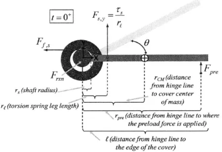
influencing the behavior of the system, it is important to draw a free-body diagram, shown in Figure 3-1. Tspring is the torque provided by the torsion spring(s) in the hinge. It drives the motion of the panel, so its sign is positive. Tp,e is the preload torque caused by kickoff spring, if present in the design. This also aids the motion of the cover, so its sign is positive. Tf,dyn is the torque caused by dynamic friction in the hinge. It always acts against the motion of the cover, so its sign is opposite that of the angular velocity. rf,stat is the torque caused by the static friction in the hinge, which acts only at the instant that the panel is deployed. This also acts against the motion of the cover, so its sign is negative. rimpacd represents the torque that is generated when the panel reaches its intended deployment angle and impacts a hard stop in the hinge. This acts against the positive motion of the panel, so its sign is negative. The full torque balance can be seen in Equation 3.2. Each term will be discussed in more detail in the following sections.

Fs=0+

F =

IF

F Abpre_rxn rc(distance

(a dfrom hinge line r, (shaft radius).to _{cover center}

of mass) rf (torsion spring leg lengt) mass)

.(distancefrom hinge line to where the preload force is applied) t (distance from hinge line to

the edge of the cover)

Figure 3-1: Free-body diagram of an item undergoing rotational motion from

3.1.1 Spring Torque

Torsion springs are generally represented by an equation of the form i- = -kO, where

positive angular displacement 9 is measured with respect to a zero-load angle,

#

0. However, in this system, the coordinate 9 is used to represent the angular displacement of the solar panel from its closed position. In this configuration, the hinge springs are oriented such that the torque provided is at a maximum when the panel is stowed and steadily decreases as the panel deploys. To account for this, the torque equation must be rewritten as shown in Equation 3.3.

rp,,,.g = nk(( - 6) (3.3)

Here, n is the number of torsion springs in the system, k is the torque constant of a single spring, 40 is the no-load angle of the torsion spring, and 6 is the deployment angle of the solar panel.

3.1.2 Preload/Kickoff Torque

For many passive deployment systems, it is common to have the mechanism preloaded when in a closed configuration. This serves the dual purpose of preventing chatter of the mechanism due to launch vibrations and providing an additional kickoff force at the moment deployment begins. This practice is advocated in the General Envi-ronmental Verification Standard [} ("GEVS") developed by NASA Goddard Space

Flight Center, which provides a set of standards for environmental testing of space hardware. Due to space constraints, none of the solar panel assemblies being studied in this thesis feature a mechanism that provides a kickoff force. However, the system whose test data is being used for model verification does have kickoff springs. For this reason, the kickoff torque term, shown in Equation 3.4, is being included in the general model.

that act near the tip of the item to be deployed. This is illustrated by the Fe term in the free-body diagram shown in Figure 3-1. Because of the short stroke of the springs, the force can be approximated as occurring instantaneously at the moment deployment begins. Mathematically, this is accounted for by multiplying the torque term by the Dirac delta function. F,e is the "preload" force acting on the stowed mechanism by the compressed springs. r,,e is the distance from the axis of rotation to the point where the kickoff force is applied.

Tpre = rreFp.eJ(t) (3.4)

3.1.3 Hinge Friction

Models for both dynamic and static hinge friction were developed by Bralower [i.]

in his modeling of a deployable door mechanism for the REXIS instrument.

3.1.3.1 Static Friction

To determine the torque caused by static friction, Bralower began by recognizing that the mechanism is in static equilibrium when in the stowed position. Therefore, the static friction in the system is directly related to the normal force required to react the force provided by the torsion spring. This term is presented in Equation 3.5 [9],

yg = r,(p~) (3.5)

where M, is the static friction coefficient of the bushing material, -r, is the total torque provided by the torsion spring(s) and r, is the torsion spring leg length.

For the bushing material used in the MicroMAS solar panel hinges, the coefficient of friction varies as a function of the contact pressure between the hinge shaft and the bushing, as depicted in Figure 3-3. The contact pressure between the shaft and bushing is a prime example of Hertz contact stress. From Budynas

[151,

the

half-width, b, of the contact area between the two parts is given by Equation 3.6. The subscript 1 denotes properties related to the shaft, and the subscript 2 denotes properties related to the bushing. E and v are the Young's modulus and Poisson's ratio, respectively, of each part; F is the contact force pushing the two parts together;

I is the length of the contact region; and d is the diameter of each part. It should

be noted that by convention, the diameter d is positive for convex cylinders. For a flat plane, d = inf. For a concave cylinder (such as a hollow tube that encompasses a shaft), d is negative. This is best illustrated in Figure 3-2.

2F (I- 4)/E + (1-4)E

b = (3.6)

Irl _{'Idi + '/4}

Once the size of the contact area is known, the maximum contact pressure can be calculated as shown in Equation 3.7. In Equation 3.5, the normal force caused by the torsion springs is calculated as r,/rI. Substituting the values shown in Table 3.1 into Equation 3.6 and Equation 3.7 yields a contact pressure of 7.87 MPa. The corresponding friction coefficient from Figure 3-31 is 0.14.

p = F (3.7)

1

I

F / ' -. -Y

tF

F 2

Figure 3-2: Hertz contact stress for two cylinders, from [

Table 3.1: Properties of hinge shaft for static Hertz contact stress analysis

di (m) 1.995 x 10-3 d2 (m) -2.054 x 10-3 E1 (Pa) 1.930 x 1011 E2 (Pa) 7.800 x 109 Vi 0.27 V2 0.45 1 (m) 6.000 x 10-3 T8 (Nm) 0.0423 r, (M) 9.750 x 10-3 As 0.14 . I

0,35 -0,30 -, :L 0,25 0 S 0,20-~ 0 *~0,10-00 5 0 O 0,00~ 0 10 20 30 40 50 60 70 80 Pressure (MPaJ

Graph 2.5: Coefficient of friction of iglidurl G as a function of the pressure

Figure 3-3: Bushing friction coefficient as function of contact pressure

3.1.3.2 Dynamic Friction

The dynamic torque in the system is dependent on the normal force at the point of contact between the hinge bushing and shaft. Bralower asserts that this force directly reacts to the centripetal force caused by the rotational motion of the cover. This term is presented in Equation 3.8 [ 1,

Tf,dn = r.(pdmrcMO2) (3.8)

where yd is the dynamic friction coefficient of the bushing material, r, is the radius of the hinge shaft, m is the mass of the panel, and rcm is the distance from the axis of rotation to the center of mass of the panel. It can be seen from this equation that the dynamic friction is a function of the square of the angular velocity, making the differential equation for the dynamics model nonlinear. It is unlikely that a closed-form analytical solution exists; approximation of the solution via numerical integration must therefore be conducted.

between the hinge shaft and the bushing while the panel is rotating. In this situation, the normal force between the two components is a function of the angular velocity, as shown by the mrCMG2 _{term in Equation 3.8. To determine this, the numerical} simulation was run once without a dynamic friction torque, to produce a worst-case estimate of the angular velocity. Furthermore, since the angular velocity changes across time, the friction coefficient does as well. The friction coefficient is inversely proportional to the contact pressure, so we will take a conservative approach and use the average value of the angular velocity to determine the friction coefficient. However, the calculation is also performed using the maximum angular velocity to gain insight into the amount this coefficient changes across the range of motion of the panel. Using the maximum value for the angular velocity, the contact pressure is 3.78 MPa, resulting in a dynamic friction coefficient of 0.24. Using the average value for the angular velocity, the contact pressure is 1.69 MPa, resulting in a friction coefficient of 0.31.

Table 3.2: Properties of hinge shaft for dynamic Hertz contact stress analysis

di (m) 1.995 x 10-3 d2 (m) -2.054 x 10-3 E1 (Pa) 1.930 x 1011 E2 (Pa) 7.800 x 109 Vi 0.27 V2 0.45 1 (m) 6.000 x 10-3 m (kg) 0.125 rCM (m) 0.113 m,~ (rad/s) 7.528 0 av, (rad/s) 3.764 Ai.xv 0.25 /2 .WV 0.31

3.1.4 Impact Modeling

The simplest method for modeling a collision between two rigid bodies is by using the theory of Hertz contact stress to determine the maximum force inside the contact region. However, this method does not account for energy dissipation during the impact [.3 , so a coefficient of restitution must be implemented to accordingly change the after-collision velocities of the two interacting bodies.

3.1.4.1 Contact Force

Though there does not exist an exact closed-form solution to the general form of the Hertz contact equation, extensive work has been done to develop approximate analytical solutions for a number of different contact area shapes. Equations for the impact force are adapted from Fabrikant [1-], who was interested in modeling the indentation depth, w, of a flat punch under an applied load, F, into an elastic plane. This is shown in Equation 3.9.

W HF (3.9)

g;T

Immediately, it can be seen that this relationship follows Hooke's Law, F = kx,

where the parameters A, g, and H act as an effective linear spring constant for the system. For our model, we are interested in determining the impact force as a function of geometry and angular displacement beyond a specified backstop angle. Therefore, Equation 3.9 must first be rearranged as shown in Equation 3.10, and then an expression approximating linear displacement from angular displacement must be determined and substituted for w.

F H (3.10)

A is the area of the contact region, which has half-side lengths a and b. To account

area term. In this study, the contact regions are all of the same shape, so a multiplier ne, will be used to represent the number of contact regions. Since a and b are half-side lengths, the area of the contact region is A = (2a)(2b) = 4ab. The full area equation

is shown in Equation 3.11.

A = nc(4ab) (3.11)

The parameter g is defined in Equation 3.12 and is specific to a rectangular region. E is the ratio of side lengths, equal to c = a/b, where a < b.

2

= (3.12)

7r[f sinh~1( ) + ---1 fsinh-'(,E)l

H, shown in Equation 3.13 is based on the material properties of the elastic plane that is being indented. E is the modulus of elasticity (Young's modulus) of the material, which influences how much the material deforms under an applied load. The term P is the Poisson's ratio for the material, which represents the percentage deformation in the two axes perpendicular to the one in which a force is applied.

H V2 (3.13)

irE

In the paper, it is assumed that the punch is perfectly rigid and the elastic plane is the only material that deforms. In reality, both the punch and the indented plane are made from elastic materials that deform under the contact force. Therefore, H needs to be modified to account for both sets of material properties. The modification is shown in Equation 3.14, where the subscripts 1 and 2 refer to the two parts that are in contact with each other. This common modification - called the "effective modulus"

-can be seen in the equations presented in the mechanical design textbooks of Budynas

1 1- v2 1-_ p

H* = I-( + )

7r El E2

(3.14)

The penetration depth, w, can be approximated from the state variable 0 during

the numerical integration. Figure Figure 3-4 shows an exaggerated version of the geometry associated with penetration of a rotational system.

/ / / / >ez~I f I / , / /

gec coco- ca~se

Rec3cm C- iA a

Acwcase-Azl ly,/O

Figure 3-4: Geometry associated with a hinged punch indenting a plane

w ~ rc(O -

OW)

(3.15)

0 is the deployment angle, 0, is the angle of the rigid backstop, and r, is the distance between the axis of rotation and the center of the contact region.

3.1.4.2 Coefficient of Restitution

The most common method of determining restitution coefficients for various types of collisions is through experimentation. At present, there does not exist a reliable way to determine this analytically [ 1. Unfortunately, 'it was not possible to conduct

the tests required to determine this parameter for the hardware being analyzed here.

However, when modeling the dynamics of the REXIS radiation cover, Bralower [ ]

conducted a series of tests against which he could correlate his models. Based on a

comparison between the relevant parameters of his system and the single solar panel

being studied here, it appears that the two systems are sufficiently similar to allow the use of his data to determine a suitable restitution coefficient. A comparison of

the relevant physical properties is provided in Table 3.3.

Table 3.3: Comparison of properties between REXIS Radiation Cover

MicroMAS Solar Panels and

An example figure showing test data for deployment in a vacuum environment at room temperature with an actuation method that provides no additional deployment torque to the system is shown in Figure 3-5. The raw data obtained from Bralower did not include angular velocity, so that had to be numerically differentiated based on the discrete angular position and time data points. This is shown in Figure 3-6.

MicroMAS REXIS

Solar Panel Radiation

Cover Mass (g) 125 54 Length (mm) 220 67 Width (mm) 82 55 IcM (kg M2 ) 5.065 x 10-4 2.020 x 10-5 Ihn (kg M2 ) 2.103 x 10-3 3.930 x 10-5 Number of 2 2 Springs Spring Free 180 180 Angle (deg) Spring Constant 1.174 x 10-4 1.693 x 10-4 (Nm/deg) III

80-0

R

Time (e)

(b) Data and correlated model for the test with a solenoid at room temperature under vacuum.

Figure 3-5: REXIS radiation cover test data

[

I

CD CD C" CD 21: , CD a OD E 0 -a_CD 0 100 80 60 40 20 U 2000 0 C -1000 E 000 0 0.05 0.1 0.15 0.2 0.25 0.3 0.35 0. Time (seconds) L n _{0.05 0.1 0.15 0.2 0.25 0.3 0.35} Time (seconds) 4 0.4

Figure 3-6: REXIS radiation cover test data with calculated angular velocity

3.1.5 Complete Equation

Combining the equations developed in Equation 3.3 through Equation 3.15 with Equa-tion 3.2, we obtain the final equaEqua-tion of moEqua-tion for a single panel system.

I-.1

++

.00k

1-I0 = nk(5o - 0) - p..mrer2(02_{) _,rn T (t) + rPeFre6(t)}

+ Timpact (3.16)

The basic equation for the impact torque was derived in section 3.1.4.1. In the case where the rotating panel impacts the backstop and is free to rebound, the impact logic is simple, as seen in Equation 3.17. The logic gets more complicated if there is a locking feature that engages at the instant the panel impacts the backstop for the first time. In this situation there are two separate impact torques, governed by different sets of parameters relating to the two contact regions.

After impacting the backstop for the first time, the locking feature is engaged and prevents the panel from rebounding. The panel then immediately impacts the locking feature, which provides a force in the opposite direction. Immediately following the impact with the locking feature, the panel again impacts the backstop. This process is repeated, dissipating energy at each impact, until the panel comes to a rest.

0, 0 < 0 < , imPaact = g n.(4ab) (3.17) 2 H* -6, > -2r, rLi(4a1 (0 - ,), < 0<,,, 7 c = Hj* (3.18) 0, 0 > 0W

In order to solve for the dynamics of a single panel with impact forces (both with and without a locking hinge), a numerical simulation has to be developed. The simulation must perform the integration of the differential equation of motion inside of a loop. After each successful completion of the integrator, the simulation must then look at the solution vector and identify the times at which the impact began and ended. It then must use the solution state at the end of impact as the initial conditions