The dynamic effects of aggregate demand and supply disturbance

Digitized

by

the

Internet

Archive

in

2011

with

funding

from

Boston

Library

Consortium

IVIember

Libraries

working paper

department

AGGREGATE DEMAND AND SUPPLY DISTURBANCE

Olivier

Jean Blanchard

Danny

Quah

by

Olivier Jean Blanchard and

Danny

Quah

*

February 1988.

*

Both

authors are with the Economics Department,

MIT,

and the

NBER.

We

thank Stanley Fischer,

Julio Rotemberg, and

Mark Watson

for helpful discussions, and the

NSF

for financial assistance.

We

are also grateful for the

comments

of participants at an

NBER

Economic Fluctuations meeting, and for the hospitality ofthe

MIT

Statistics Center.

by

Olivier Jean Blanchard and

Danny

Quah

EkonomicB Department,

MIT.

February 1988.

Abstract

We

decompose

the behavior of

GNP

and unemployment into the dynamic effects oftwo types of shocks: shocks that have a permanent effect on output and shocks that do not.

We

interpret the

£rst as supplyshocks, thesecond as

demand

shocks.

We

£nd

that

demand

disturbanceshave a

bump

shaped effecton both output and

unemploy-ment; the effectpeaks aftera yearandvanishes after two to three years.

Up

to ascaJefactor, the

dynamic

effecton unemployment of

demand

disturbancesis amirrorimageofthaton output.

The

effectofsupplydisturbanceson outputincreasessteadilyovertime, toreach a

peak

after twoyears

and a plateau after five years. "Favorabie" supply disturbances

may

initially increase

unemploy-ment.

Thb

is followed by a decline in unemployment, with a slow return over time to its original

value.

Whilethisdynamiccharacterizationisfairlysharp, thedataarenot as specificasto the relative

contributions of

demand

and supply disturbances to output fluctuations. Wis find that the time

series ofdemand-determined output Buctuations haspeaks and troughs which coincide with

most

ofthe

NBER

troughsandpeaks. But variancedecompositions of output at various horizons giving the respective contributions ofsupply and

demand

disturbances are not preciselyestimated. For

instance, at aforecast horizon of fourquarters,

we End

that, under alternative assumptions, the

Introduction.

In response to an innovation in

GNP

of 1%, one should revise one's forecast

by more

Ihan

1%

over long horizons. This fact is

documented

by Campbell and

Mankiw

{1987a), building on earlier

work

by Nelson

and Plosser (1982).

What

doesthis statistical fact

mean

formacroeconomics? Iftherewere only one

main

typeofdisturbance

in the economy, its implications would be clear; all

we

would need to do

would

be to find

what

those

disturbances are, and

why

their

dynamic

effects have the shape characterized by

Campbell

and

Mankiw.

But

if, as is likely,

GNP

is affected by more than one main type of disturbance, say by aggregate

demand

and by aggregate supply disturbances, the interpretation becomesmoredifficult. In thatcase, the univariate

moving

average representation of output is a combination of the dynamic response of output to each of

the two disturbances. Clearly, knowing only the aggregate effect does not allow us to recover those two

responses.

Campbell

and

Mankiw

show

that their estimated univariate representation for

GNP

is equally consistent with, forexample, eitherwhite noise productivitygrowth andsmall, short-lived, effectsof

demand

disturbances on

GNP,

orinstead, with serially correlatedproductivity growthand larger, serially correlated,

effects of

demand

disturbances.

We

are interested in investigating the dynamic effects ofdisturbances that have only transitory impact

on output as well as ofdisturbances that havepermanent impact. Studies that impose strict

random

walk

behavior in the

permanent component

are necessEirily incapable ofaddressing this issue (and

we

feelstrongly

that this is the interesting characterization to obtain). Allowing the permanent

component

to have rich

serialcorrelation however destroysidentification to aprofound extent:

Quah

(1988) shows

how

any general

difference stationary process can always be decomposed into permanent and transitory

components

where

the

components

are orthogonal at allleads and lags, and such that the varianceofthe first difference ofthe

permcinent

component

is arbitrarily close to zero.

To

proceed, one

must

eitherimpose additional a priorirestrictionson the response ofoutput to each of

the disturbances, oruse information from time seriesother than

GNP,

andestimate a multivariate

represen-tation.

The

first approach hasbeenfollowedin Clark (1987a), and

Watson

(1986)

among

others. Thispaper

ako

been taken in Clark (1987b), Campbell and

Mankiw

(1987b), and Evans (1986); our approach differs

mainly inits choice ofidentifyingrestrictions. Notsurprisingly,

we

findourrestrictions

more

appealingthan

theirs.

Our

approach isconceptually straightforward.

We

eissume that thereare twokinds ofdisturbances.

We

assume that neither has a long run effect on unemployment.

We

assume however that the first has a long

run effect on output while the second does not. These assumptions are sufficient to just identify the two

typesof disturbances, their time series and theirdynamic effectson output and unemployment.

WhUe

the disturbances are defined bythe identification restrictions,

we

believethat they can be given

a simple economic interpretation.

We

think of the disturbances that have a long run effect on output as

being mostly productivityshocks.

We

think of the disturbancesthat have no such longrun effect as being

mostly non-productivity-induced

demand

disturbances.

We

find this interpretation useful and reasonable,

as wellas supported by the results of the paper. Forshort, (and

we

hope, not too misleadingly)

we

refer to

these types ofdisturbances as aggregate supply and aggregate

demand

disturbances respectively.

Under

these identificationrestrictionsand thiseconomic interpretation,

we

obtain the following

charac-terization of fluctuations:

demand

disturbances have a

hump

shaped effect on both output and

unemploy-ment; theeffect peaks after a year and vanishesafter two to three years.

Up

to ascale factor, the dynamic

effect on

unemployment

of

demand

disturbances is a mirror image of that on output.

The

effect of supply

disturbances on output increases steadily overtime, toreach a peak aftertwoyears and aplateau Eifter five

years. "Favorable" supply disturbances

may

initially increase unemployment. This is followed

by

a decline

in unemployment, with a slowreturn over time to its originalvalue.

While this

dynamic

characterization is fairly sharp, the data are not as specific as to the relative

contributions of

demand

and supply disturbances to output fluctuations.

On

the one hand,

we

find that

the time series ofdemand-determined output fluctuations, that is the time series of output constructed by

puttingallsupply disturbance realizations equalto zero, haspeaks and troughswhich coincide withmost of

the

NBER

troughs and peaks. But,

when we

turn tovariance decompositionsofoutput atvarious horizons,

we

findthattherespectivecontributionsofsupply and

demand

disturbancesare notpreciselyestimated. For

4

of

demand

disturbances rangesfrom 30 to 80%.

The

paper has five sections. Section 1 discusses identification. Section 2 discusses our economic

inter-pretation of the disturbances. Section 3 discusses estimation. Section 4 characterizes the

dynamic

effects

of

demand

and supply disturbances on output and unemployment. Section 5 characterizes the relative

contributions of

demand

and supply disturbances to fluctuations in output and

unemployment.

1. Identification.

We

assume that there are two types of disturbances affecting

unemployment

and output.

The

first heis no

long run effect on either

unemployment

or output.

The

second has no long run effect on unemployment,

but

may

have a long run effect on output.

We

assume further that these disturbances are uncorrelated at

allleads and lags. These restrictions in effect define the two disturbances. As indicated in the introduction,

and discussed at length in the next section,

we

refer tothe first as

demand

disturbances and to the second

as supply disturbances.

We

now

discuss

how

these restrictions identifj- the two disturbances and their

dynamic

effects. Let

Y

and

U

denote the logarithm of

GNP

and the level of unemployment, respectively. As will be clear below,

our assumptions imply that the first difference of

Y

,

AY,

and the level ofunemployment, U, have a jointly

stationary bivziriate autoregressiverepresentation:

D{L)Xt

=

vt, where D(0)

=

I and E{vtvl)

=

n

(l)

where

X

denotes the

2x1

vector

\AY

U]'.

The

matrix polynomial in lag operators

D{L)

is of order n,

with all determinantal roots outside the unit circle.

The

white noise bivariate vector sequence t; is serially

uncorrelated, with v

=

[vy _vu] •

Under

our assumption that there are two types ofdisturbances in the economy,

demand

and supply,

equation (1) is the reduced form of a

model

which describes the dynamic effects of those disturbances on

outputand unemployment.

The

vectorvcomprisesreducedformdisturbances, whichare linearcombinations

ofthese

demand

andsupply disturbances.

By

specifying the reduced form as above,

we

have already imposed a

number

of restrictions on the

unemplojTnent; this implies in turn that neither ofthe two types ofunderlying disturbances has a long run

effecton unemployment.

By

contrast,since itisthe firstdifference andnot thelevelofoutputwhichappears

inequation (1),

we

have allowed both reducedformdisturbances, andthusboth

demand

and supply, tohave

a long run effect on the levelofoutput.

The

only restriction that

we

have not yet imposed is that

demand

disturbances haveno longruneffect on output. This isthe key assumption thatwill allowus to identifythe

demand

and supply disturbances, and to recover interpretable dynamics from the reduced form.

We

now

show

how

it is used.

The

first step is to obtain the moving average representation of the reduced form. Multiplying both

sides ofequation (1) by

D[L)~^

gives:

Xt

=

C{L)vt, where C(L)

=

D{L)-\

so that C{0)

=

I. ₍₂₎

On

the other hand, the moving averagerepresentation corresponding toour

demand

and supply disturbance

model

is:

Xt

=

A{L)ct (3)

where Ct is the vector of

demand

and supply disturbances, Cf

=

[cdt e.t] , with e^t being the

demand

disturbanceande,t the supply disturbance. Giventhe assumptionthat

demand

andsupply disturbancesare

uncorrelated,

we

can without lossofgenerality take the covziriancematrixofe tobe theidentitymatrix.

The

condition that

demand

disturbances haveno long run effect on output implies that aii(l)

=

in equation

(3). In words, the coefficients on current and lagged

demand

disturbances in the output growth equation

must

sum

to zero.

We

now show

that our modelis just identifiedfrom the estimated reduced form.

Combining

equations

(2) and (3) gives:

Xt

=

A[L)et

=

C{L)vt, where C(0)

=

/, and E[vtv't)

=

CI.

Thus, our

model

isjust identified ifand onlyifthere exists a unique matrix

S

such that Set

=

^t and

SS'

=

n, and A{L)

=

C[L)S

and aii(l)

=

0.

The

first conditionstates that

5

is a square root ofthe covariance matrixofthe reducedform disturbances:

6

column

of S. This is the fourth restriction neededfor identification. That restriction is given explicitly by:

<:ii(l)sii

+

ci2{l)s2i

=

0.

There always exists a unique matrix

S

that satisGes these restrictions.''^

Identification is thus achieved by using a long runrestriction. This raises a knotty technical issue. It

is well-known that, in the absence of precise prior knowledge of lag lengths, inference and restrictions on

asymptotic behavior of the kind

we

are interested in here is delicate.^

More

precisely, viewed in terms of

Fourier transforms, the restriction immediately above operates on a zero measure interval of the range of

frequencies, and so is especially suspect. It is easy howeverto generalize this restriction to one that applies

to

some

5-neighborhood of frequency zero, and then to perform estimation in the frequency domain.

By

imposing that the restriction holds overa frequencyband,

we

would be using anoveridentifyingrather than

just identifying restriction.

Under

appropriate regularity conditions,

we

can

show

that our results are the

limit of the results fromfrequency domain estimation, as S tends to zero.

In

summary,

our procedure is as follows.

We

first estimate the reduced form, equation (l), and derive

its

moving

average representation, equation (2).

We

then construct the matrix S, and use it to recover the

moving

average representation of the

demand

and supply disturbance model, equation (3).

^

_The

_{proof is as follows. First obtain the Choleski factorization of}

Cl.

Then

any matrix .S is an

or-thonormal transformationof the Choleski matrix.

The

restrictionon the first

column

imposed by aii(l)

=

determines the orthonormal transformation uniquely, up to column sign chcinges. This is the

method

we

actually use to construct S.

See for instance Sims (1972).

We

are extrapolating here from Sims's results which assume strictly

exogenous regressors.

We

conjecture that similar problems arise in the

VAR

case. If anything, one would

Interpreting residuals in smalldimensionalsystems as "structural" disturbances is always perilous, and our

interpretation ofdisturbances assupply and

demand

disturbajices is noexception.

We

discussvariousissues in turn.

Grantingour assumption thatthe

economy

is affected by two main types of disturbances, productivity

and non-productivity-induced

demand

shocks, one

may

reasonably argue that even

demand

disturbances

havelong runeffectson output: changes in the subjectivediscountrate,orchanges infiscal policy

may

well

affect the saving rate and the longrun capital stock and output.

The

presence of increiising returns, and of

learning bydoing, also raises the possibilitythat all

demand

shocks

may

have

some

longrun effects.

Even

if

theydonot, their effects throughcapitalaccumulation

may

besufficientlylong lasting to beindistinguishable

from truly permanent effects in the sample.

We

believe that

demand

shocks

may

well have such long run

effects on output.

To

the extenthowever that the long runeffects of

demand

shocks are small

compared

to

that of supply shocks, a proposition

we

consider reasonable, our decomposition is "nearly correct" in the

following sense: in a sequence ofeconomies where the sizeof the long run effect of

demand

shocks becomes

arbitrarilysmallrelativeto that ofsupply, the correct identifyingscheme approaches that which

we

actually

use. This is

shown

in the technical appendix. This proposition is the ajialogue in our context to the "near identification" proposition in traditional approachesto identification.

Granting our assumption that the

economy

is affected by two

main

types of disturbances, one with

permanent

effects on output, the other only with transitory effects, alternative interpretations are possible:

following Prescott (1987), one might instead view the

economy

as being affected by two types of supply

disturbances,

some

withpermanent and

some

with transitory effectsonoutput.

Our

identifyingassumptions

willthenidentify thosetwodisturbances. Whilethisisnot ourprefered interpretation,

we

shall brieflydiscuss ourresults underthat alternative interpretation below.

This raises a final set ofissues constituting problems inherent in estimation and interpretation ofany

low dimensional

dynamic

system. Suppose that, there are in fact

many

sources of shocks, each of

them

having different

dynamic

effects on output and unemployment. Clearly, if there are

many

supply shocks,

8

with permanent and

some

with transitory effects on output, and ifthey all play an equally import2int role

in aggregate fluctuations, our decomposition is likely to be meaningless.

A

more

interesting case is that in

which aUormost supply shocks havepermanenteffects onoutput, and allor

most

demand

shockshaveonly

atransitoryeffectonoutput.

One

might hopethat, in this case,ourprocedure is able todistinguish correctly

the

dynamic

effectsof

demand

disturbancesfromthose ofsupplydisturbances. This isunfortunately nottrue

in general.

We

show

this explicitly in the technical appendix, where

we

establish necessary and sufficient

conditions for this separation to occur.

From

the reasoning in the technical appendix,

we

also see that

there are important sets of circumstances under which our procedure does correctly identify the different

effects of

demand

and supply. Roughly speaking, the different components in output and

unemployment

must

bear a stable

dynamic

relation to each other, across the individual

demand

disturbances and across the

individualsupply disturbances.

Thus

ifthere isonly one supplydisturbance, and thereis a stableproduction function confronting the different

demand

disturbances, ourprocedure correctly isolates the

dynamic

effects

of

demand

and supply disturbances. This particular set ofconditions

we

find to be not at allunreasonable.

To

summarize, our interpretation ofshocks is subject to various caveats.

We

believe it neverthelessto

be reasonable, and to be supported by the results presented below.

We

now

briefly discuss the relation ofour paper to otherson the

same

topic.

We

first examine

how

our

approachrelates tothe business-cycle-versus-trend distinction :

Following estimation,

we

can construct two output series, a series reflecting only the effects of supply

disturbances, obtained by setting allrealizations ofthe

demand

disturbances to zero, and a series reflecting

only theeffectsof

demand

disturbances, obtainedbysettingsupplyrealizations tozero.

By

construction,the

firstseries, the supply

component

ofoutput,willbe non-stationary while the second, the

demand

component,

is stationary.

By

construction also, the two series are uncorrelated.

A

standard distinction in describing output

movements

is the "business cycle versus trend" distinction.

Whilethereisno standard definitionofthese components, thetrendisusually takento be that partofoutput

that would realize, were all prices perfectly flexible; business cycles are then taken to be the dyncimics of

actual output around its trend. ^

It is tempting to associate the first series

we

construct with the "trend"

component

of output and the second series with the "business cycle" component. In our view, that association is unwarranted. If prices

are in fact imperfectly flexible, deviations from trend will arise not only from

demand

disturbances, but

alsofrom supplydisturbances: business cycles willoccur dueto both supply and

demand

disturbances. Put

another way, supply disturbances will affect both the business cycle and the trend component. Identifying

separately business cycles and trend is likely tobe difficult, asthe twowillbe correlated through theirjoint

dependence on current and past supply disturbances.

With

this discussion in mind,

we

now

review the approachesto identification used byothers.

Campbell and

Mankiw

(1987b) assume the existence oftwo types ofdisturbances, "trend" and "cycle"

disturbances, which are assumed to be uncorrelated. Theiridentifying restriction is then that trend

distur-bances do not affect unemployment.

The

discussion abovesuggests that this assumption of zero correlation

between cycle and trend components is unattractive; iftheir two disturbances are instead reinterpreted as

supply and

demand

disturbances respectively, the identifying restriction that supply disturbances do not

affect

unemployment

is equally unattractive.

Clark (1987b) also assumes the existence of "trend" and "cycle" disturbances, and also assumes that

"trend" disturbances do not affect

unemployment

but allowsfor contemporaneouscorrelation betweentrend

andcycle disturbances. While thisis an improvementoverCampbell and

Mankiw,

it stillseverely constrains

the

dynamic

effectsof disturbances on output and

unemployment

in ways that are difficult to interpret.

The

paper closest to ours is that ofEvans (1986). Evans assumes two disturbances, "unemployment"

and "output" disturbances,which can be reinterpreted assupply and

demand

disturbances respectively.

By

assuming the existenceofareducedform identicaltoequation (1) above, he alsoassumes that neithersupply

nor

demand

disturbanceshavea long run effect on unemployment, butthat both

may

have a longruneffect

on thelevelofoutput. However, instead ofusing the longrun restriction that

we

use here, he assumes that

supply disturbances have no contemporaneous effect on output.

We

find this restriction less appealing as a

way

ofachieving identification; it should be clear howeverthat our paper builds on Evans' work.

imperfect information, this would be the path of output, absent imperfect information. In models with

nominal rigidities, this would be the path of output, absent nominal rigidities. In models that assume

market clearing and perfect information, such as Prescott (1987), the distinction between business cycles

10

S.

Estimation.

One

final problem needs to be confronted before estimation.

The

representation

we

use in equation (l)

assumesthatboth the levelof

unemployment

and the first difference ofthe logarithmof

GNP

are stationary

around given levels.

The unemployment

data suggest however a small secular increase in

unemployment

over the post

war

period in the US. This raises a

number

ofissues.

One

possibility is that, in fact,

unemployment

is permanently affected

by

either supply or

demand

disturbances, or by both. This might occur iffor example the

economy

were characterized by the type of

hysteresiB studied by

Summers

and coauthor (1986).* This would require an altogether different modeling

approach.

We

do not consider it further here.

A

second possibility is that there are, in addition to

demand

disturbances, two types of supply

distur-bances.

The

first, which might include changes in productivity, has long run effects on output but not on

unemployment.

The

second, which might include changes in the composition of the labor force, changes in

search technology and so on, does have long run effects on unemployment. If this is the case, one strategy

wouldbe to postulatethe existence ofthose three disturbances, onefrom

demand

and two from supply, and

characterizetheir

dynamic

effects. This issubstantially

more

difficultthan

what

we want

to do.

A

short cut,

acceptable ifequilibrium

unemployment

drifts slowlythrough time, isto allowfor a deterministic time trend

in unemployment. This is

what

we

do below, by first regressing

unemployment

on a linear time trend and

using the residuals to estimate equation (1).

The

estimated time trend implies an increase in equilibrium

unemployment

of 3.6% over the post

war

period. As

we

find this estimate to be high,

we

report three sets

ofresults, those obtained removing this estimated trendfrom

unemployment

(which

we

shallcall the "trend

removed" casebelow), those obtainedremoving a trendwith slope equalto half oftheestimated value ("half

trend removed"), and those obtained not removing any trend ("no trend removed").

We

estimate equation (l) using quarterly dataforreal

GNP

and the aggregate

unemployment

ratefrom

1950-2to 1987-2.

We

presentthe results ofestimation allowingforeightlags.

(We

performedestimation with

twelve lags with little difference Ln the results.

We

also experimented with estimating the system omitting

the first fiveyears, as the

Korean

War

eraseems anomalous. Again, the empiricalresults remain practically

unchajiged.)

The

system is the same as that estimated by Evans, with alonger sample;

we

referthe reader

to Evansfor a description ofthe characteristics ofthe estimated autoregressive system..

We

directly turn to

interpreting the dynamiceffects ofsupply cind

demand

disturbances.

4.

Dynamic

effects of

demand

and

supply

disturbances.

The dynamic

effects of

demand

and supply disturbances are reported in Figures 1 and 2. These figures

correspond to the case where half of the estimated unemployment trend is

removed

from

unemployment

before estimation of the jointprocess.^

The

corresponding figures for the other two cases are for the most

partsimil2ir, and are givenin theAppendix. Differencesbetween the three setsof results willbepointed out

in the text.

The

upper part of Figure 1 gives point estimates of the dynamic effects of a

demand

disturbance

on output and unemployment.

The

scale for the logarithm of output is given on the left, the scale for

unemployment

on theright. Similarly, the lower part ofFigure 1 givespointestimates ofthe

dynamic

effects

ofa supply disturbance on

Y

and U. Figure 2 again provides pointestimates ofthe

dynamic

responses, but

now

with one standard deviation bands around those estimates.®

Demand

disturbances have a

hump

shaped effect on output and unemployment. Their effects peak

after 2 to 4 quarters, depending on the treatment ofthe

unemployment

trend.

The

effects of

demand

then

decline tovanish after8 to 14 quarters.

The

size of theeffect on outputis largest inthecase

when

the trend

in

unemployment

is fullyremoved.

The

responses in output and

unemployment

are mirror images ofeach

other;

we

return to this aspect of theresults below after discussing the effectsof supply disturbances.

These dynamiceffects are consistentwith a traditioneJview ofthe dynamic effectsofaggregate

demand

on output and unemployment, in which

movements

in aggregate

demand

build

up

until the adjustment of

prices and wagesleads the

economy

backto equilibrium.

Supply disturbances have an effect on the level of output which cumulates steadily over time.

The

We

have chosen to present the figures for this case in the text not because

we

like it best but simply because the results are -not surprisingly- in between those ofthe two other cases.

More

precisely, these figures give the square root of

mean

squared deviations from the point estimate

in 1000 bootstrap replications. Thus, the bands need not be and indeed are not symmetric. In every case,

entire pseudo-histories are created by drawingwith replacement from the empiricaldistribution ofthe

VAR

mnovations. These calculations were performed using a combination of

RATS

and S on a

Sun

workstation

responses

to

demand

CD

d

CNJ

d

C\J

d

to

--0.5

10

20

30

40

responses

to

supply

m

d

LO

d

LO

10

20

30

40

output

response

to

demand

output

response

to

supply

CM

o

^

CM

q

?\

LO CO

o

>

'l CD ' \'^

d

_q

^

v.\

o

-;. \ C\J

d

-

w

\

IT) > •

\

d

\ /• \ ^ C\J 1 1 1 1 1 1 1 1 1

q

d

o

/• • •

/•

_'•...

/• ^V, 1- ' /• _/

^-

_{_}

• ^ ,' / / / / 1 , 1 1 1 . J 1 u

10

20

30

40

10

20

30

40

unempi

response

to

demand

unempi

response

to

supply

o

d

CM

d

d

CD

d

CM

d

o

d

CM

d

d

10

20

30

40

10

20

30

40

12

peak response is about two to three times the initial effect aind tiikes place after eight quarters.

The

effect

decreases tostabilize eventually at twothirds of its peak value.

The

dynamic response in

unemployment

is

quite different: a positivesupply disturbance (thatis, asupply disturbance thathas a positivelongruneffect

on output)

may

initially increase

unemployment

slightly. Ifthis increase occurs, the effect is reversed after

a few quarters, and

unemployment

slowly returns to its originalsteady state value.

The dynamic

effects of

a supply disturbance on

unemployment

are largely overby about five years.

The

response of

unemployment

and output Eire suggestive of the presence of rigidities, both nominal

and real. Nominal rigidities can explain

why

in response to a positive supply shock, say an increase in

productivity, aggregate

demand

does not initially increase enough to

match

the increase in output needed

to maintain constant employment;real

wage

rigidities can explain

why

increases in productivitycan lead to

a decrease Ln

unemployment

after a few quarters, which persists until real wages have caught up with the

new

higher levelof productivity.

Figure 1 alsosheds interestinglighton the relation betweenchangesin

unemployment

and output

known

as Okun's Law. In our sample, a regression of annual percentage changes in output on annual changes in

unemployment

yields acoefficient of-2.4, the absolutevalue ofwhich is

known

as Okun's coefficient.

Under

our interpretation,this coefficient isa mongrelcoefficient, as thejointbehavior ofoutput and

unemployment

depends on the type of disturbance affecting the economy. In the case of

demand

disturbances. Figure 1

suggests that there is indeed a tight relation between output and unemployment.

The

absolute value ofthe implied coefficient is roughly equal to 2, lower than Okun's coefficient. In the case ofsupply disturbances,

there is no such close relation between output and unemployment. In the short run, output increases,

unemployment

may

riseorfall; inthe long run, outputremainshigherwhereas by assumption

unemployment

returns to its initial value. In the intervening period,

unemployment

and output deviations are ofopposite

sign, and the absolute value of the implied coefficient is close to 4, higher in absolute value than Okun's

coefficient. That the absolute value of the coefficient is higher for supply disturbances than for

demand

disturbances isexactly

what

we

expect. Supplydisturbances arelikelyto affect the relation between output

and employment, and to increase output with little or no change in employment.

two disturbances

we

have isolated were in fact both supply disturbances, the first having only temporary

effects, the second havingpermanent effects, and that all marketscleared under perfect information.

What

interpretation could be given to the djTiamic responses given in Figure 1?

Temporary

productivity

distur-bances shouldlead tostrong intertemporalsubstitutioneffectson labor supply, and thisclearly couldexplain

the behavior of output and

unemployment

in the upper part of Figure 1.

As

permanent disturbances to

productivitycumulateovertime, this could explain the dynamiceffects ofthe disturbanceson output in the

lower part of Figure 1.

The

anticipation ofhigher productivity later would induce workers, in reaction to

apositive innovation in productivity, to intertemporally substitute

away

from current

work

towardwork in

the future; thiswould explain the initial increase and the subsequentdeclinein unemployment. Thus, in the

absence ofmore information, the dynamiceffects presentedin Figure 1 are clearly susceptible to alternative

Output

fluctuations

absent

Demand

CO C\J CO

o

CO CO r-* CO ->;};

o

1950

1960

1970

1980

1990

CD

O

CM

O

o

CD

O

Output

fluctuations

due

to

Demand,

Unemployment

fluctuations

absent

Demand.

1950

1960

1970

1980

1990

Unemployment

fluctuations

due

to

Demand,

CO OJ

o

C\J CO

1950

1960

1970

1980

1990

14

5. Relative contributions of

demand

and

supply

disturbances.

Having

shown

the

dynamic

effects of each type of disturbance, the next step is to assess their relative

contribution to fluctuations in output and unemployment.

We

do this in two ways.

The

first is informal,

and entails a comparison of the historical time series of the

demand component

of output to the

NBER

chronology of business cycles.

The

second examines variance decompositions of output and

unemployment

in

demand

and supply disturbances at various horizons,

a.

Demand

distwrbcinceB and

NBER

buBiness cycles.

PYom

estimation ofthejoint processfor output and unemployment, and our identifying restrictions,

we

can

compute

the

demand

componentsofoutput and unemployment. These are the time paths ofoutput and

unemployment

thatwould have obtainedin theabsenceofsupply disturbances. Similarly, bysetting

demand

innovations to zero,

we

can generate the time series of supply components in output and unemployment.

From

the identifying restriction that

demand

disturbances have no longrun effect on output, the resulting

series of the

demand

component

in the level of output is stationary.

By

the

same

token, both the

demand

and supply components of

unemployment

are stationary.

The

time series corresponding to the "half-trend removed" case ispresented in Figures 3 (output) and

4 (unemployment).

The

upper panel presents the historical supply component, the lower panel presents the

historical

demand

component. Superimposed on these time series are the

NBER

peaks and troughs. Peaks

are

drawn

as verticallines above the horizontal axis, troughs as vertical lines below the axis.

Allthreeassumptions about the trend in

unemployment

yield qualitativelysimilarresults.

The

demand

component

is quite large, approaching

5%

on each side ofthe origin. (The

demand

component

is larger on

average in the "trend removed" case.)

The

peaks andtroughsofthe

demand component

in outputmatchclosely the

NBER

peaks and troughs.

The

tworecessions of 1974-1975 and 1979-1980 deserve specialmention.

Our

decomposition attributes

them

in about equal proportions to adverse supply and

demand

disturbances. This is best

shown

by giving the

73-3 73-4 74-1 74-2 74-3 74-4 75-1 Cd -0.1 0.2 -0.8 0.9 -1.4 -1.2 -3.0 e. -1.6 -0.1 -1.0 -1.1 -1.4 0.4 1.2 79-1 79-2 79-3 79-4 80-1 80-2 Cd -0.7 1.1 0.3 -0.4 -0.4 -3.1 e. -0.6 -2.0 0.5 -0.9 0.9 -0.9

The

recession of 1974-75 istherefore explainedby aninitial string ofnegativesupply disturbances, and then

of negative

demand

disturbances. Similarly, the 1979-80 recession is first dominated by a large negative

supply disturbance, and then alarge negative

demand

disturbance. Without appearing to interpret every

single residual,

we

find these estimated sequences of

demand

andsupply disturbances quite plausible.

It

may

also simply be that the supply disturbances of these two periods were different from typical supply disturbances, such as changes in productivity, which dominate the sample.

They

had a stronger

short-run contractionary effect, with both declines in output and increases in unemployment.

As

a result,

they

may

look

more

like

demand

disturbancesunderouridentification restrictions, andarethereforeclassified

as

demand

disturbances.^

Notice that the supply component in output, presented in the upper panel in Figure 3, is clearly not a

deterministic trend. It exhibits slowergrowth in the late 1950's, as wellas in the 1970's.

Figure 4 gives the supply and

demand

components in unemployment (the time trend is added back

to the supply component).

Unemployment

fluctuations due to

demand

correspond closely to those in the

demand

component

of

GNP.

This is consistentwith our earlier finding on the mirror image

moving

average

responses of

unemployment

and output growthto

demand

disturbances.

The model

attributes substantial

fluctuation in

unemployment

to supply disturbances, again with increases in the late 1950's and aroundthe

time ofthe oil disturbances ofthe 1970'e.^

This suggests extending the analysis to incorporate information from another variable.

That

variable

would be chosen so that it itself is likelyto react differently to supply and

demand

disturbances. Obvious

candidates wouldbe the price level orthe relative price ofraw materials. In Blanchard and

Watson

(1986), evidencefromfourtimeseriesisusedto decomposefluctuations intosupplyand

demand

disturbances. There

the recession of1975 is attributed in roughly equal proportions to adverse

demand

andsupply disturbances, that of 1980 mostly to

demand

disturbances. In view of those results,

we

reestimated the model, leaving out 1973-1 to 1976-4.

The

estimated dynamic effects ofboth demeind and supply disturbances were nearly identical to those described above.

By

construction, the supply

component

of

unemployment

is close to actual

unemployment

for the first

few observations in the sample. Thus, the large decreasefrom 1950 to 1952in the supply

component

simply

reflects the actual

movement

in

unemployment

in this period. In light of this,

we

re-estimated the model from 1955-2 through the end ofour sample.

We

found little change in the empiricalresults.

16

b. Variance decompositions.

While the above empirical evidence is suggestive, a

more

formal statistical assessment can be given by

computing variance decompositions for output and

unemployment

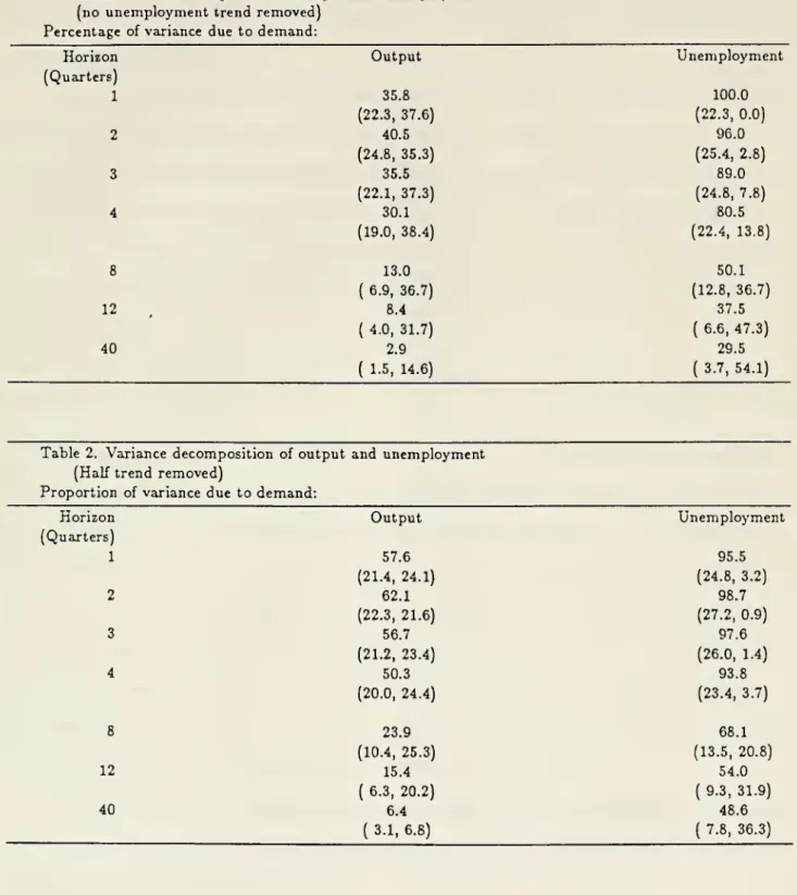
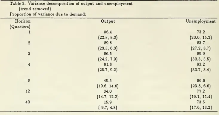
at various horizons.

Tables 1 through 3 give those variance decompositions, under the three alternative assumptions about

the

unemployment

trend. Thesetables havethe following interpretation. Define the k quarter-aheadforecast

error in output as the difference betvifeen the actual value of output and its forecast from equation ₍₁₎ as

of k quarters earlier. This forecast error is due to both unanticipated

demand

and supply disturbances in

the last k quarters.

The number

for output at horizon k,k

=

1,...,40 gives the percentage ofvariance of

the /c-quarter ahead forecast error due to demand.

The

contribution of supply, not reported, is given by

one hundred minus that number.

A

similar interpretation holds for the

numbers

for unemployment.

The

numbers

in parentheses are standard deviations.°

The

results are given for all three assumptions about the

unemployment

trend, as there are important differences across these alternative hypotheses.

Our

identifying restrictions impose only one restriction on the variance decompositions, namely that

the contribution ofsupply disturbcinces to the variance of output tends to unity as the horizon increases.

All other aspects are unconstrained.

Two

main

conclusions emerge from these tables.

First, the datado not give a precise answerastotherelativecontributionof

demand

and supply distur-bances to

movements

in output at short and

medium

term horizons.

The

results vary with the treatmentof

the

unemployment

trend: the relative contributionof

demand

disturbances, fourquarters ahead, rangesfrom

30%

(no trendremoved) to

82%

(trend removed);eight quarters ahead, it stillranges from

13%

to 50%.

The

reason for this

may

be seen by comparing Figure 1 with the corresponding Figures in the Appendix, derived

under alternative assumptions about the

unemployment

trend. While they are qualitatively similar, the

effects of

demand

disturbances are smaller, and the effects ofsupply disturbances are stronger and quicker,

in the "no trendremoved" case.

Even

for a given assumption about trend, the standard deviation bands are large. For example, in

the "half trend removed" case, the one standard deviation

band

on the relative contribution of

demand

(no

unemployment

trend removed)

Percentageofvariance dueto demand:

Horizon (Quarters) 1 2 3 4 8 12 40 Output 35.8 (22.3, 37.6) 40.5 (24.8, 35.3) 35.5 (22.1,37.3) 30.1 (19.0, 38.4) 13.0 ( 6.9, 36.7) 8.4 ( 4.0, 31.7) 2.9 ( 1.5, 14.6)

Unemployment

100.0 (22.3, 0.0) 96.0 (25.4, 2.8) 89.0 (24.8, 7.8) 80.5 (22.4, 13.8) 50.1 (12.8, 36.7) 37.5 ( 6.6,47.3) 29.5 ( 3.7, 54.1)

Table 2. Variance decomposition ofoutput and unemployment

(Half trend removed)

Proportion ofvariance due to demand:

Horizon (Quarters) 1 2 3 4 8 12 40 Output 57.6 (21.4, 24.1) 62.1 (22.3, 21.6) 56.7 (21.2, 23.4) 50.3 (20.0, 24.4) 23.9 (10.4, 25.3) 15.4 ( 6.3, 20.2) 6.4 ( 3.1, 6.8)

nemployment

95.5 (24.8, 3.2) 98.7 (27.2, 0.9) 97.6 (26.0, 1.4) 93.8 (23.4, 3.7) 68.1 (13.5, 20.8) 54.0 ( 9.3, 31.9) 48.6 ( 7.8, 36.3)

Table 3. Variance decomposition ofoutput and

unemployment

(trendremoved)

Proportion of variance due todemand:

Horizon Output

Unemployment

(Quarters) 1 86.4 73.2 (22.8, 8.3) (20.0, 15.2) 2 89.8 83.7 (23.5, 6.3) (27.2, 8.7) 3 86.5 89.9 (24.2, 7.9) (30.3, 5.5) 4 81.8 93.2 (25.7, 9.2) (30.7, 3.4) 8 49.5 86.6 (19.6, 14.6) (23.8, 6.6) 12 34.0 77.2 (14.7, 12.2) (19.1, 11.4) 40 15.9 73.5 [17.6, 13.2)

disturbances four quarters ahead ranges from

30%

to 75%. Eight quarters ahead, it stillranges from

14%

to 49%. At longer horizons, the contribution of

demand

disturbances goes to zero by construction; it is

typically small afterfour years.

The

secondmain conclusion is that the contribution of

demand

disturbances to

unemployment

is more

substantial and more precisely estimated, at short and

medium

term horizons. In all three cases,

demand

disturbances contribute between

80%

and

90%

of the variance of

unemployment

four quarters ahead; their

contribution, eight quarters ahead, varies between

50%

to 87%.

The

one standard deviation

band

in the

"halftrend removed" caseranges from

60%

to

98%

fourquarters ahead, andfrom

55%

to

89%

eightquarters

ahead. There is considerable uncertainty as tothe relative contribution of

demand

and supply disturbances

at long horizons.

6.

Conclusion.

We

have assumedthe existence oftwotypes ofdisturbances generating

unemployment

and output dynamics,

the first typehavingpermanenteffectsonoutput, thesecond having only transitoryeffects.

We

have argued

that these two types of disturbances could usefully be interpreted as productivity and non-productivity

induced

demand

shocks respectively, or,for short, as supply and

demand

shocks.

Under

that interpretation,

we

have concluded that

demand

disturbances have a

hump

shaped effect on output and

unemployment

which disappears after approximately two to three years, and that supply disturbances have an effect on

output which cumulates overtime to reach a plateau afterfiveyears.

We

have also concluded that

demand

disturbances

make

a substantial contribution to output fluctuations at short and

medium

term horizons;

however, the data do not allow us to quantify this contribution with great precision.

Our

identifying restrictions allow us to ask interesting questions ofthe

dynamic

effects of disturbances

that have permanent effects. These questions cannot be addressed by studies that restrict the permanent

component

to be apure

random

walk.

While

we

find thissimple exercise tohave been worthwhile,

we

also believe that further

work

isneeded,

especially to validate andrefine our identification ofshocks as supply and

demand

shocks.

We

have in

mind

18

supply components of

GNP

with a larger set of macroeconomic vaxiables. Preliminary results appear to confirm our interpretation of shocks.

We

find in particular the supply

component

of

GNP

to be strongly positively correlatedwith realwagesathigh to

medium

frequencies,whilenosuchcorrelationemergesforthe

demand

component.^"

The

second extensionistoenlarge thesystem toone infourVciriables,

unemployment,

output, prices and wages. Thiswould re-examine the empirical questionsin Blanchard (1986), by using the

long run identification restriction developed in this paper. This extension appears important; one would

expect that

wage

and price data will help identify more explicitly supply and

demand

disturbances.

The

methodology and results will be described in a future paper.

The

statement in the text refers to

the

sum

of correlations from lags -5 to

+5

between the supply innovation derived in this paper and the innovations inreal wages obtained from univariate

ARIMA

estimation.

TechnicalAppendix

This technicalappendix discusses further and establishes the claims

made

in the section on

interpreta-tion.

First,

we

asserted in the text that our identification scheme is approximately correct even

when

both

disturbances have permanent effectson the levelofoutput, provided that the long-run effect of

demand

on

output is small.

We

now

prove this.

The

first element of the model, output growth, has the moving average representation in

demand

and

supply disturbances:

AV;

=

aii(L)edt

+

ai2(i)e,<

where aii(l) is the cumulative effect on the level of output

Y

of the disturbance ej.

The

moving average

representationC{L), together with theinnovation covariancematrix fl, isrelatedtoour desired interpretable

representation through

some

identifying matrix S, such that:

SS'

=

n, and A{L)

=

C{L)S.

The model

is identified by choosing a unique identifying matrix S. In the paper,

we

selected the unique

matrix

S

suchthat aii(l)

=

0.

Let the long-run effect ofthe

demand

disturbance be 6 instead, where 6

>

without loss of generality.

For eachS, thisimplies adifferentidentifyingmatrixS(S). Let |S'((5)-.S(0)|

=

maxy,*: (5'y*:((5)

-

5'yfc(0)) ; this

measuresthe deviation in the implied identifying matrix from that which

we

use. Since the approximation

is thus seen to be a finite-dimensionalproblem, any matrix

norm

willinduce the

same

topology,which isall

that is needed to study the continuity properties of our identification scheme. All of the empirical results

vary continuously in

S

relative to this topology. Thus, it is sufRcient to

show

that

|5'(<f)

-

5(0)1

—

as ,5

—

0.

Inwords,ifan

economy

has long-runeffects in

demand

that aresmall but different fromzero, ouridentifying

scheme which incorrectly assumes the long-run effects to be zero nevertheless recovers approximately the

20

We

prove this as follows. Since both 5(0) and S(6) are matrix square roots of Cl, there exists an

orthogonal matrix

V

[6) such that:

S(6)=S(0)V(S),

y/here

V[S)V(Sy

=

I.

Then

the long-run effectof

demand

is the (1, 1) element in the matrix;

A{1;6)

=

C(l)S{6)

=

C{l)S(0)V(6).

But

recall that the elements of the first row of C(l)5(0) are respectively, the long-run effects of

demand

and of supply on the level of output,

when

the long-run effect of

demand

is restricted to be zero.

Thus

for any V{S), the

new

implied long-run effect of

demand

is simply the long-run effect ofsupply (under our identifying assumption that the long-run effect of

demand

is zero) multiplied by the (2,2) element of the

orthogonal matrix V[6). As 6 tends to eero, the _(2,2) element of V{6) tends continuously to zero as well.

But, up to a column sign change, the unique

V

[S) with (2,2) element equal to zero is the identity matrix.

This establishes that S[6)

—

» 5(0), element by element. Hence,

we

have

shown

that \S[S)

—

₅₍₀₎|

—

» as S-* 0. Q.E.D.

Next,

we

turn tothe effectsofmultiple

demand

and supply disturbances: Suppose that there is z. _pd"x1

vectorof

demand

disturbances fdt, and a p, x 1 vectorofsupply disturbances f,t, so that:

\Ut

_J

-

V^2:(L)'

B22(Lyj

{f,tj

where B-jk are column vectors of analytic functions; Bji has the

same

dimension as /j, Bj2 has the

same

dimension as /,, and Bii{z]

=

(1

—

z)Pii{z), for

some

vector of analytic _{functions fin.}

Each

disturbance

has a different distributed lag effect on output and unemployment.

Since our

VAR

method

allows identification of only as

many

disturbances as observed variables, it is

immediate that

we

will not be able to recover the individual components of /

=

(/^ /^)'.

To

clarify the issues involved,

we

provide an explicit example where our procedure produces misleading

results. Supposethatthereisonlyone supply disturbanceand two

demand

disturbances: fdt

=

{fdi,t,

affects only unemployment.

The

supply disturbance affects both output and unemployment. Formally,

assume that the true model is:

An

unrestricted

VAR

representationcorresponding to this data generating process is found by applying the

calculations in

Rozanov

(1965)

Theorem

10.1 (pp. 44-48). (A slightly

more

readable discussion of those

calculations

may

be found in EssayIV in

Quah

(1986).)

The

implied moving average representationis:

1 1

-(^

_^'V")"'

^-'-'-It is straightforward to verify that the matrix covariogram implied by this

moving

average matches that of

the true underlying model. Further, the unique zeroof the determinant is 2, and consequently lies outside

the unit circle. Therefore this moving average representation is, as asserted, obtained from the vector autoregressive representationofthe true model.

However,this

moving

average does notsatisfyouridentifyingassumption thatthe

"demand"

disturbance

has onlytransitoryeffectsonthelevelof output.

We

thereforeapplyouridentifyingtransformationtoobtain:

This

moving

average representation is

what

we

would recover if in fact the data is generated by the three

disturbances [fdi, jd2> /.)• Notice that while the supply disturbance /, affects both output growth and

unemployment

equally and only contemporaneously,

we

would identify e, to have a larger effect on output

than on unemployment, together with a distributed lag effect on output. Further a positive

demand

dis-turbance, restricted to have only a transitory effect on output, is seen to have a contemporaneous negative

impact on unemployment. In the truemodelhowever,no

demand

disturbances affect output and

unemploy-ment

together, either contemporzmeously or at any lag. In conclusion, a researcherfollowing our bivariate

procedure is likely to be seriouslymisled

when

in fact the true underlying

model

is driven by more than two

disturbances. Havingseen this,

we

ask under

what

circumstanceswill this mismatchin the

number

of actual

and explicitly modeled disturbances be benign?

22

Theorem:

Let

X

be a bivariate stochastic sequence generated by

(i.)

X,

=

5(L)/t ;

(ii.) ft

=

(fat f',t)'. with /d pd X 1, /. p. X 1 ;

(iii.) Eftft-k

=

I if A;

=

0, and otherwise ;

(v.) B,,{z)

=

[\-z)p,,[z);

(vi.) pii, B21, B12, B22 are column vectors ofanaJyticfunctions;

_Pn

and B21 Pd x 1, -^12 aiid ^22 P« X 1 ,'

fvii.j

55*

isfuiiranJc on \z\

=

1, wiiere* denotescomplex conjugation followed by transposition.

Then

there exists a bivariate

moving

averagerepresentation forX, Xt

=

A[L)et, such that:

(viii.) A[z)

—

{ ^^, I ^^1

\ ], **'j"ti

°ni

^12) ^121) '^22 scalar functions, detyl

^

for all \z\

<

1;

y021(2] 022(2)/

(ix.) 011(2)

=

(1

—

z)qii(2), with Qii analytic on \z\

<

1; and

(x.) Ct

=

\ I, EtfCt-k

=

I

ifk

=

Q, and is otherwise. \e.t J

In the bivariate representation, e^ is orthogonal to _f,, and t, is orthogonal to fd, at aJiieads and Jags

ifand onlyifthere exists a pairofscalarfunctions 71, 72 such that:

B21

=

li. •_/i5ii,

622

=

I2 B12.

Conditions (i.) - (vii.) describe the true data generating process fortlie observeddata in output growth

and unemployment. There axe _pj

demand

and p, supply disturbances; (v.) expresses the requirementthat

demand

disturbances have only transitory effects on the ievei of output. Condition (vii.) is a regularity

condition that allows the existence of a

VAR

mean

square approximation.

The moving

average recovered

by our

VAR

procedure is described by (viii.) - (x.): the

Theorem

guarantees that there always exists such arepresentation.

The

second part ofthe

Theorem

establishes necessary andsufficient conditionsonthe underlying model

such that the bivariate identification procedure does not inappropriately confuse

demand

and supply

in output growth and unemployment axe sufficiently similcir across the different

demand

disturbances, and

across the different supply disturbances. This doesnot

mean

thatthe dynamic responsesin output growth

and

unemployment

across

demand

disturbances must be identical or proportional, simply that they differ

up

to a scalar lag distribution.

Thus

even though in general a bivariate procedure is misleading, there are important and reasonable

sets ofcircumstances under whichour techniqueprovides the "correct" answers. Forinstance, suppose that there is only one supply disturbance but multiple

demand

disturbances. Suppose further that each ofthe

demand

components in the level of output has the same distributed lag relation with the corresponding

demand

component

in unemployment. This cissumption is consistentwith our 'production function'-based

interpretations below.

Then

our procedurecorrectly distinguishes thedynamiceffects of

demand

andsupply

components in output and unemployment.

Proof

of

Theorem: By

(i.) - (vs.), thematrixepectriLldensityof

X

isgiven bySx{i^)

=

5(z)5(z)*|, .j.

By

reasoninganalogous to that in pp.44-48 in

Roianov

(1965), there exists a 2 x 2 matrixfunction C, each

ofwhose elements are analytic, with det

C

_^

for \z\

<

1, and

Sx

=

CC

on \z\

=

1. This represents

X

as a

moving

average in unit variance orthogonal white noise, obtainable from its

VAR

mean

square

approximation.

However

such a

moving

average

C

need not satisfy the condition that the first (demand)

disturbancehave only transitoryimpact on the levelofoutput (condition (ix.)).

Form

the

2x2

orthog-onaJ

matrix

M

whose second columnis the transpose of the Brst

row

of

C

evaluatedatz

=

1, normalized tohave

length 1, as a vector. Then

A

=

CM

provides the

moving

average representation satisfying (viii.) - (x.).

For thesecond part ofthe Theorem, notice that

A

has been constructed so that on \z\

=

1:

|1

-

zHaiip

+

lai^r

=

|1

-

_{^r^li (^li)'}

+

B[, {B[,)' ;

(1

-

z)aiia*i

+

aisa'j

=

(l

-

z)^[^ (B^

J*

+

B[^

(S^J*

;

ksiP

+

|a22|2

=

_5^1 (S2i)*

+

5^2(522)*.

Fore<f to be orthogonalto/,, ande, to be orthogonal_{to f^} at allleadsandlags, itisnecessaryandsufficient

tiat on \z\

=

1:

(a.)

_{\a,,\^=P[AP[S;}

24

(c.) aiiaji

=

fi'ii

[B2S

;

(d.) 012022

=

-012 (-^22) >

(f.) \a22?

=

B!,^(B'^^y.

Considerrelations (a.), (c), and (e.). Denoting complexconjugation of

B

by B, the triangle inequality

implies that:

j=i y=i

where the inequality is strict unless B21 is a complexscalarmultiple of

_Pn

for each z on \z\

=

1. Next, by

the Cauchy-Schwasz inequality,

again y/ith strict inequality except

when

B21 is a complex scalar multiple of

_Pn,

for each z on \z\

=

1.

Therefore:

|aiia2il^

^

lo^iil^ • ^22^, on \z\

=

1,

where the inequality is strict except

when

B21 is a complex scalar multiple of fin on |r|

=

1. But tiie

strictinequalityis a contradiction as

an

and 022 axe just scaiar/"unctions.

Thus

(a.), (c), and (e.) can be

simultaneously satisSedifandonlyifthereexists

some

complexscalarfunction')i{z) such that B21

=

7i

-^ii-A

similar argument applied to (b.), (d.), and (f.) shows that they can hold simultaneously if

and

only if

there exists

some

complex scalar function ')2(^] such that B22

=

72 Bi2- This establishes the Theorem.

responses

to

demand

CD

O

d

CM

o

10

20

30

40

responses

to

supply

LO LO

d

LO

d

LO

10

20

30

40

responses

to

demand

Ln

o

o

o

un

o

LO * • _ \ /• \ / \ / S f

0.1

0.0

-0.1

-0.2

-0.3

-0.4

-0.5

-0.6

10

20

30

40

in LO CJ

o

o

LO

O

responses

to

supply

LO

10

20

30

40

References

Blanchard, Olivier, "Wages, Prices, and Output:

An

Empirical Investigation,"

mimeo

MIT,

1986. Blanchard, Olivier and

Mark

Watson, "Are businesscycles allalike?" in

"The

American business cycle;

continuity and change", R. Gordon ed,

NBER

and University ofChicago Press, 1986, 123-156.

Cochrane, John,

"How

big isthe

random

walkcomponent in

GNP

?", forthcoming Journai ofPolitical

Economy

1988.

Campbell, J.Y. and N.G. Mankiw, 'Are Output Fluctuations Transitory?" Quarteriy JournaJof

Eco-nomics,

November

1987, 857-880.

Campbell, John and N. Gregory Mankiw, "Permanent and transitory components in macroeconomic

fluctuations",

AER

Papers and Proceedings,

May

1987, 111-117 (b).

Clark, P.K. , "The Cyclical

Component

in

US

Economic Activity," Quarter/y Journai ofEconomics,

November

1987, 797-814 (a).

Clark, Peter, "Trendreversioninrealoutputandunemployment",forthcoming Journai of Econometrics,

1987 (b).

Evans, George, "Output and

unemployment

in theUnited States", mimeo, Stanford, 1986.

Nelson, CharlesandCharles Plosser, "Trends£ind

random

walksinmacroeconomic timeseries". Journal of

Monetary

Economics, September 1982, 10, 139-162.

Prescott, Edward, "Theory aheadofbusiness cyclemeasurement".Federal Reserve

Bank

of Minneapolis QuarterlyReview, Fall 1986, 9-22.

Quah, Danny, "Essays in

Dynamic

Macroeconometrics", Ph.D. dissertation, 1986, Harvard University.

Quah, Danny, "The RelativeImportance ofPermanent and Transitory Components: Identification and

Some

Theoretical Bounds," mimeo,

March

1988,

MIT.

Rozanov,

Yu

A., Stationary

Random

Processes, 1965, San Francisco: Holden-Day.

Sims, Christopher, "The role ofapproximate prior restrictions in distributed lag estimation". Journal

ofthe American StatisticalAssociation,

March

1972, 169-175.

Summers,

Lawrence and Olivier Blanchard, "Hysteresis and European

Unemployment",

Macroeco-nomics Annual, 1986, 15-78.

Watson, Mark, "Univariate detrending methods with stochastic trends". Journal of

Monetary

Date

Due

G-^-e'^

''lu^

_12%