SWIM: the first spaceborne wave scatterometer

HAL Id: insu-01456490

https://hal-insu.archives-ouvertes.fr/insu-01456490

Submitted on 29 Mar 2017

HAL is a multi-disciplinary open access

archive for the deposit and dissemination of sci-entific research documents, whether they are pub-lished or not. The documents may come from teaching and research institutions in France or abroad, or from public or private research centers.

L’archive ouverte pluridisciplinaire HAL, est destinée au dépôt et à la diffusion de documents scientifiques de niveau recherche, publiés ou non, émanant des établissements d’enseignement et de recherche français ou étrangers, des laboratoires publics ou privés.

Danièle Hauser, Céline Tison, Thierry Amiot, Lauriane Delaye, Nathalie

Corcoral, Patrick Castillan

To cite this version:

Danièle Hauser, Céline Tison, Thierry Amiot, Lauriane Delaye, Nathalie Corcoral, et al.. SWIM: the first spaceborne wave scatterometer. IEEE Transactions on Geoscience and Remote Sensing, Institute of Electrical and Electronics Engineers, 2017, 55 (5), pp.3000-3014. �10.1109/TGRS.2017.2658672�. �insu-01456490�

Abstract—This paper provides an overview of the SWIM

(Surface Waves Investigation and Monitoring) instrument which will be one of the two payload instruments carried by CFOSAT (China France Oceanography SATellite) with a planned launch date in mid-2018. SWIM is a real aperture wave scatterometer operated at near-nadir incidence angles and dedicated to the measurement of directional spectra of ocean waves. The SWIM flight model is currently being assembled and tested, its performance is being assessed and its prototype data processing algorithm is being developed. The aim of this paper is to provide a complete overview on the motivations and scientific requirements of this mission, together with a description of the design and characteristics of the SWIM instrument, and the analysis of its expected performances based on a pre-launch study. An end-to-end simulator has been developed to evaluate the quality of the data products, thus allowing the overall performance of the instrument to be assessed. Simulations run with two subsets of full orbit subsets show that the performances of the instrument and the inversion algorithms will meet the scientific requirements for the mission.

Index Terms— radar, radar applications, radar

cross-sections, remote sensing, satellite applications, sea surface.

I. INTRODUCTION

Ocean surface wind and waves are key parameters affecting the marine meteorology,

ocean dynamics, the ocean/atmosphere

exchanges, as well as marine resources, pollution, global economics and safety (navigation, fisheries, offshore structures, harbor, tourism…), and coastal environments (sedimentation, pollution). Due to the synoptic scales of the processes governing these parameters, there is strong need for them to be monitored continuously on a global scale, thereby allowing not only operational oceanography to be implemented [1], but also enabling improved modeling and a better understanding of the coupled ocean/atmosphere system to be achieved [2]. The international panel of the GOOS (Global Ocean Observing System) organization has identified the sea-state parameters as essential

variables for reliable climate monitoring1. They also note that there is very few possibility to measure wave parameters at the global scale, beyond the significant wave height.

In this context, the Chinese and French Space Agencies (resp. CNSA and CNES) have agreed to jointly develop an innovative mission, referred to as CFOSAT (China France Oceanography SATellite). It aims at monitoring simultaneously ocean surface wind and waves at feeding related science and applications. CFOSAT has been designed to serve the operational needs of meteorological and marine forecasting and their associated applications, together with international research objectives (wind-wave interactions, wave interactions with currents, wave impact on sea-ice, air-sea fluxes, wave climate,...). CFOSAT will also provide the scientific community with the opportunity to complement the data retrieved by other satellite missions, for the estimation of land surface parameters (soil moisture and roughness in particular), and for the measurement of polar ice sheet characteristics.

With respect to previous or existing missions, CFOSAT will innovate by contributing more comprehensive information related to ocean waves (full directional spectra of ocean waves for swell wind-sea, and mixed conditions), and by providing simultaneous and co-located observations of wind and waves. To achieve these objectives, the CFOSAT payload comprises two radar instruments: SWIM (Surface Waves Investigation and Monitoring), a wave scatterometer operated at near-nadir incidence to measure the directional spectra of surface waves, and SCAT, a wind scatterometer operated at

1 _(see

http://www.goosocean.org/index.php?option=com_content&view=article& id=14)

SWIM: the first spaceborne wave scatterometer

medium incidence, allowing the ocean surface wind vector to be measured.

Presently, global observations of ocean surface waves are rather limited. They are provided either by altimeter missions or by SAR missions. But the only wave parameter provided by radar altimeter missions is the total significant wave height [3], with no information concerning the dominant direction of propagation or wavelength of the waves. Although operational assimilation of altimeter products into numerical wave forecast models is implemented since the 1990’s (see e.g [4]), it is now recognized that the inclusion of these data has only a limited impact on the performance of wave forecasting, as a consequence of the lack of spectral information [5]. As for SAR observations, although SAR images can be processed to retrieve the directional spectra of waves, the measurement principle based on the analysis of Doppler information in the backscattered signals, restricts the retrieved information to the longest waves (generally longer than 250 m in wavelength) and/or to waves travelling in a direction more or less perpendicular to the satellite ground track. This is due to the so-called “azimuth-cutoff” effect resulting from the random motion of sea surface scatterers [6, 7, 8]. As a consequence, the separation of the processing steps necessary for SAR data inversion, for ocean wave spectra assimilation, and for numerical wave prediction is possible only in swell conditions [8, 9]. Despite these limitations, spectral information related to the swell, including its unambiguous direction of propagation [10], is very helpful when it comes to monitoring swell properties far from its generation zone [11], improving the physical parameterization of models [12], and/or improving the performance of swell forecasts [13, 5]. However, as a result of SAR limitations, there are a number of sea state conditions where little or no spectral information is available: wind-sea and the initial stages of swell, and crossed seas with wind-sea. Furthermore, one of the remaining challenges is to upgrade the accuracy of measurements of wave propagation direction and directional spread, in order to improve our understanding and modeling of the influence of currents, small islands, and icebergs, etc.

The SWIM instrument has been designed with a real-aperture azimuth-scanning geometry, in order to determine the directional spectra of ocean waves, without the limitations of SAR imaging mechanisms. Spectral information associated with oceanic waves will thus be accessible, not only under long-swell conditions, but also in mixed sea and wind-sea conditions, with a high azimuthal resolution. When compared to satellite SAR observations, the drawback of SWIM is that wave spectra will be obtained with a spatial resolution of several tens of kilometers only (of the order of 90 km), as opposed to that of 10 to 20 km obtained with space-borne SAR measurements.

Although ocean surface winds are now well monitored on the global scale, through the use of satellites with either scatterometer, SAR, or microwave radiometer payloads, there is a lack of simultaneous and co-located observations of wind and waves. The CFOSAT mission, with its dual payload comprising the wave scatterometer SWIM and the wind scatterometer SCAT, will open up new opportunities, in particular for the study of wind and wave interactions at the regional scale, or for the improved tracking of waves radiating from large storms. In addition, with its multi-incidence configuration, SWIM will provide new information on sea-surface roughness for the case of both short and long waves.

The CFOSAT mission makes use of a polar orbit, at an altitude of 519 km. A 13-day cycle was chosen in order to ensure global coverage of directional wave spectra on this time scale (the swath characteristics are described in section IV). In the case of the SCAT instrument, thanks to the use of a larger swath, global coverage will be achieved in just 3 days. The system will continuously gather and download data via two polar stations (French component) and three mid-latitude stations (Chinese component). The polar stations (Inuvik-Canada and Kiruna-Sweden) will provide the system with a near-real time transmission and processing capability (i.e. within

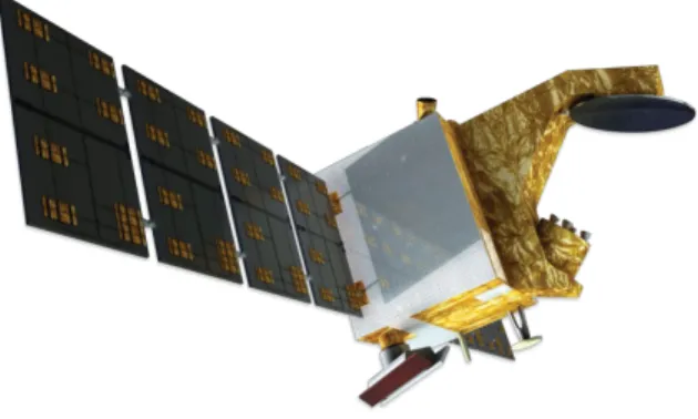
less than 3 hours after acquisition), to allow assimilation processes and forecast procedures to be implemented by atmospheric or marine operational forecast centers. Two mission centers (one Chinese and one French) will independently process all of the data from both payloads. The CFOSAT launch is now planned for mid-2018. Figure 1 provides an artist’s view of the satellite with its two payloads, which are both Ku-band instruments (operating at 13.6 GHz and 13.2 GHz, respectively) scanning around the vertical axis:

- the wave spectrometer SWIM operates at near-nadir incidence angles with 6 beams that cover the [0°-10°] incidence range and scan conically over 360° in azimuth,

- the wind scatterometer SCAT operates at medium to large incidence angles (26° to 46° from nadir) using a fan-beam conically scanning antenna [14].

Figure 1. Artist’s view of the CFOSAT satellite. The SWIM feed horns and antenna are mounted on the right-hand panel, and the SCAT

antenna is mounted on the bottom panel. The other antennas on the Earth-facing panel are for TM/TC (X and S-bands). © CNES/ Gekko.

This present paper focuses on the SWIM instrument. Details of its measurement concept and scientific requirements are provided in Section II and III, respectively. In Section IV, the main characteristics and performances of the instrument are presented. In Section V, the ground-based data processing is explained, some examples of simulated directional wave spectra are illustrated, and performances on the retrieved parameters are discussed, based on observation simulations. A summary is given in Section VI.

II. MEASUREMENT CONCEPT

SWIM is designed to measure the 2D wave spectrum, i.e. wave height or wave slope density spectrum of as a function of the 2D wavenumber vector k. We first recall that this spectrum is defined as the Fourier Transform of the instantaneous spatial autocorrelation of surface displacements:

𝐸 𝒌 = _%&$ % 𝑍 𝒖 𝑒*+,𝒖_𝑑𝒖

𝒖 (1)

where Z(u) is the two-dimensional

autocorrelation function of the surface elevation, and u is the 2D horizontal vector.

In the following, polar coordinates are used and the 2D wave height spectrum is noted as E(k,j), where k is the modulus of the wavenumber vector and f is the direction of wave propagation. The wave slope spectrum F(k, j) is related to the wave height spectrum by:

F(k,j) = k2_E(k,f)

(2) The total energy of the wave height spectrum is characterized by the significant wave height Hs, written as:

𝐻_/ = 4 _{, 4} 𝐸 𝑘, 𝜙 𝑘𝑑𝑘𝑑𝜙 (3)

The concept of SWIM is based on a scanning-beam real-aperture radar. It was proposed in the 1980’s by Jackson et al., both for airborne and spaceborne configurations [15, 16. 17], in order to avoid the limitations of SAR imaging, in terms of the retrieval of directional spectra of ocean waves. This concept has been implemented and validated on various airborne systems such as the Ku-band Radar Ocean Wave Spectrometer (ROWS) developed by Jackson et al. [17], the C-band system RESSAC [18], the C-band polarimetric system STORM [19]. More recently the Ku-band KuROS airborne radar [20], was specifically designed to prepare the CFOSAT mission, under a configuration as similar as possible to that of SWIM (Ku-Band, similar incidence range). The results show that the concept is sufficiently

mature to be transposed onto a satellite. Although a preliminary design for a spaceborne instrument was established more than fifteen years ago [21], SWIM will be the first spaceborne instrument based on this principle.

The physical principles used to measure directional ocean wave spectra with a real-aperture azimuthally scanning radar are presented in [16, 17, 18] and recalled in the following, with emphasis being placed on the analytical equations which are the basis of the data processing algorithms. These principles are general and do not depend on the type of platform (aircraft or satellite). But the specifications for the geophysical products and for the design of the instrument (presented in section III and IV) apply to our chosen satellite configuration with the SWIM instrument.

The measurement principle relies on the fact that at near-nadir incidence (around 8°-10° from nadir), the normalized radar cross-section is sensitive to the local slope of the sea surface, which is related to the tilt of long waves, but is almost insensitive to small scale roughness effects produced by the wind, and to hydrodynamic modulations resulting from interactions between short and long waves.

For each azimuthal direction j of the antenna, a position on the mean sea surface can be defined by its local horizontal coordinates x and y, where x is the distance along the antenna pointing direction, and y is the distance along the

azimuthal direction. The elementary

backscattering cross-section s is given by s = s0A, where A is the area contained within a radar range gate. The presence of surface of long waves (longer than the resolution cell) produces a tilt modulation of s given by:

δσ(x, y) =σ(x, y) −σ(x, y) (4)

where σ_{(x, y) is the mean surface radar}

cross-section which would occur if no large-scale waves were present. This cross-section depends only on the small-scale roughness, with a

relatively small influence over this range of incidence angles.

As shown in [16], the fractional variation of the normalized radar cross-section along the direction of wave propagation is:

δσ σ ≅ cotθ − ∂lnσo ∂θ $ % & ' ( )∂ζ ∂x (5)

where ∂z/¶x is the local slope of the surface in the direction of wave propagation.

Using a real-aperture radar, the fractional modulation m(r,f) of the cross-section seen by the radar is averaged laterally across the beam:

𝑚 𝑟, 𝜙 = 789: ;,< => ?,@

> ?,@ A<

789: ;,< A< (6)

where Gaz is the beam width antenna pattern, σ is the backscattering coefficient, r is the radial distance, q is the incidence angle and f is the azimuthal direction.

The polar-symmetric slope spectrum k2_{E(k,f) is} related to the spectral density of modulation Pm(k,f) by: 𝑃_C 𝑘, 𝜙 = 𝛼𝑘%_{𝐸(𝑘, 𝜙) (7)} where 𝛼 is: 𝛼 = _G%& H 𝑐𝑜𝑡𝜃 − NOPQR NS % (8) In the above expressions, the tild notation indicates that the variable is taken at the center of the footprint; Ly is a length related to the azimuthal width of the beam footprint:

𝐿_U = V X89

% % OP% (9)

where R is the radial distance and baz the 3dB azimuthal beam width. Note that Eq. (8) is valid when it is assumed that the antenna gain pattern is near Gaussian, and that Ly is much greater than the wavelength to be detected. The latter

assumption is necessarily satisfied in the case of a space-borne configuration. Here, the function <a> is called the Modulation Transfer Function (MTF).

Eq.8 shows that the parameter <a> is related to the mean trend of s0 as a function of incidence angle. Assuming the backscattering to be quasi-specular [22], this dependence on incidence angle is inversely proportional to the mean square slope (mss) of the sea surface. As the sea surface mss is dominated by the shortest waves, it is sensitive mainly to wind speed and <a> thus decreases when the wind speed (or mss) increases. This theory also predicts that the sensitivity of <a> to wind speed is the greatest at low to moderate wind speeds (0-10 m/s). The TRMM/PR data confirm this trend [23]. They also show that <a> varies with significant wave height for a given wind speed, but this remains a second order effect [23] when compared to the sensitivity of <a> to wind speed.

In the absence of speckle and thermal noise effects in the signal fluctuations, the spectral density of signal modulations due to waves Pm(k,f) can be derived from the measurements as:

Pm(k,φ) = 1

2π m(x,φ)m(x +ξ,φ) e

−ikξ_dξ

∫

where m(x,f) is determined for each radar azimuthal direction f as the projection onto the surface of the signal modulation m(r,f), and the brackets denote an ensemble average.

In reality, thermal and speckle noise may affect the signal fluctuations. The influence of thermal noise on signal fluctuations can generally be ignored, thanks to a strong-signal-to-noise ratio (SNR). The influence of speckle noise can be minimized by using a wide transmission bandwidth, and by averaging independent samples in space (over successive range gates) and/or time (temporal integration). However, a trade-off must be found between the space and time domains of integration, and the specification of wavenumber cutoff and azimuthal resolution

for the wave spectra. As a consequence, the signal fluctuations arising from speckle may not be completely negligible when compared to the modulations produced by long waves, such that in the spectral domain, the relationship between signal modulation and surface wave slope modulation (neglecting the effects of thermal noise) is:

𝑃YQZ 𝑘, 𝜙 ≈ 𝛿 𝑘 + 𝑃^V 𝑘 𝑃C 𝑘, 𝜙 + 𝑃/_ 𝑘 (11)

where Psp is the density spectrum of the signal fluctuations due to speckle, PIR is the density spectrum of the impulse response, 𝛿 is the Dirac function, and 𝑃_YQZ is the density spectrum of the signal fluctuations: P_δσ 0(k,φ) = 1 2π δσ0(x,φ)δσ0(x +ξ,φ) e −ikξ_dξ

∫

By assuming the pulse shape to be approximated by a Gaussian function, PIR(k) can be expressed as:

𝑃_^V(𝑘) = 𝑒𝑥𝑝 − _𝟐𝑲𝒌𝟐 𝒑

𝟐 (13) where Kp is related to the ground-projected resolution δX:

𝐾_{_} =𝟐 𝒍𝒏𝟐

𝜹𝑿 (14)

Using the same assumptions, the speckle density spectrum can be expressed as:

(15) where Nsp is the number of independent samples used to estimate the signal intensity.

III. SCIENTIFIC REQUIREMENTS

The scientific requirements for the

SWIM/CFOSAT mission were established, taking into account the need for a breakthrough with respect to existing space-borne instruments, the € P_sp(k) = 1 2πKpNsp e − k 2 2Kp2

need to develop improved numerical wave models, and the potential for contributing new information with respect to that provided by in

situ measurements. The main specification of

SWIM is thus to generate directional spectra of ocean waves for all wavelengths greater than approximately 70 m, in order to provide the scientific community with data related not only to swell conditions, but also to wind sea and mixed sea conditions. Resolution in wavelength and direction have been specified to be of the order of (for wavelength) or better (for direction) than that of wave buoy measurements, and compatible with equivalent frequency and directional resolutions in numerical global wave models. Note however, that the proposed directional resolution of 15° has never been achieved with in situ measurements, although it corresponds to the wave direction resolution of the standard wave models. The accuracy of wave energy (or significant wave height) was required to be of the same order of magnitude as that provided by standard wave buoys. As for the spatial sampling required for directional spectra, the 5 to 10 km resolution normally available with space-borne SAR cannot be achieved when conical scanning is used. For these reasons, the spatial resolution requirement was chosen to be close to that of the global wave models (of the order of 50 km to 100 km). Useful information can thus be brought for wave model validation and/or the assimilation of data into wave forecast models. As for the nadir products, the requirement is similar to that of current satellite altimeter missions.

In agreement with these scientific requirements, the instrument and data processing have been designed to deliver the following products and accuracies:

- Wind and wave parameters from nadir measurements:

• significant wave height better than 10% or 50 cm (maximum),

• wind speed accuracy of approximately ± 2 m/s or 10% (whichever is greatest), - Directional wave spectrum from off-nadir

measurements:

• Two-dimensional wave spectra

estimated at a scale of 70 km x 90 km, • Wavelengths detected from 70 m to 500

m,

• Dominant wavelengths with an

accuracy of 10%, for up to three partitions of the wave spectrum,

• Dominant directions with an accuracy of 15°, for up to three partitions of the wave spectrum,

• Significant wave height accuracy better than 10%, for up to three partitions of the wave spectrum.

IV. SWIM TECHNICAL DESCRIPTION

A. Overview of the instrument

In order to achieve the above requirements, a specific instrument has been designed. Its main characteristics are inherited from the RESSAC [18], STORM [19], and SWIMSAT [21] concepts. SWIM is a Ku-band real aperture radar, which illuminates the Earth's surface at six different incidence angles: 0°, 2°, 4°, 6°, 8° and 10°, with a beam width of approximately 2°. In the case of nadir observations, the concept is very similar to that of the most recent altimeter missions [24]. In order to acquire data in all azimuthal directions, the antenna feed horns are rotated continuously at 5.6 rpm. Using this

geometry, SWIM allows the following

geophysical parameters to be measured:

- Normalized radar cross-section for incidence angles in the range between 0° and 10° (all beams combined),

- Significant wave height and sea surface wind speed (determined using the nadir beam),

- Directional ocean wave spectra (from the 6°, 8° and 10° beams, hereafter referred to as “the spectrum beams”).

With respect to the concepts initially proposed in [16], and the specifications first defined in [21], SWIM will produce data at multiple, off-nadir incidence angles (see Fig 4.a). This will provide improved along-track sampling of the directional

spectra (see Fig 4b below), as well as continuous profiles of the normalized radar-cross-section for incidence angles between 0 and 10°. These measurements will allow the tilt MTF and the wave spectra to be computed. They will also allow the wind speed and (under optimal conditions) direction to be determined, and will contribute to further studies of the sea surface slope probability density function [25, 26, 27], as well as to the development of continental applications.

When compared to an airborne design based on the same concept, the main challenge for SWIM is to ensure homogenous conditions at the scale of the swath dimension. These requirements led to the choice of a low Earth orbit (altitude 519 km), and to a design with three off-nadir beams for the measurement of directional wave spectra. Moreover, in order to estimate the tilt MTF from the data, incidence angle coverage of the order of 10° or more is required. In contrary to the case of an airborne instrument, this range of incidence angles is greater than that required to estimate the wave spectrum itself. The rapid motion of the satellite along its ground track also leads to strong constraints on speckle noise reduction. It requires to choose a suitable trade-off between on-board noise reduction (by averaging over time and space) and post-processing, including speckle density spectrum estimation and elimination.

1) Main parameters

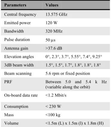
Table I summarizes the main parameters of the instrument. These were chosen as a result of various trade-offs between signal-to-noise ratio, swath and footprint dimensions, geometrical constraints, speckle minimization, data rate limitations, and platform constraints. Note that the chosen bandwidth corresponds to an intrinsic range resolution of 0.47 m, which is then degraded by the on-board averaging.

TABLEI MAIN SWIM PARAMETERS

Parameters Values Central frequency 13.575 GHz Emitted power 120 W Bandwidth 320 MHz Pulse duration 50 µs Antenna gain >37.6 dB Elevation angles 0°, 2.3°, 3.7°, 5.55°, 7.4°, 9.25° 3dB beam width 1.5°, 1.5°, 1.7°, 1.8°, 1.8°, 1.8° Beam scanning 5.6 rpm or fixed position

PRF Between 5.0 and 5.4 k Hz

(variable along the orbit) On-board data rate <1.2 Mbit/s

Consumption < 230 W

Mass <100 kg

Volume <1.5m (L) x 1.5m (l) x 1.8m (H)

2) Architecture

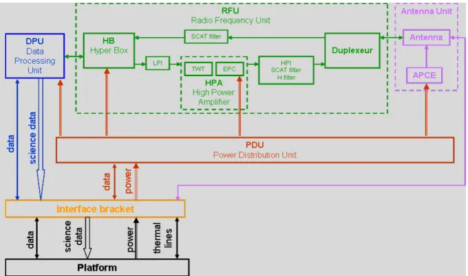
The architecture of the instrument is summarized in Fig. 2.

SWIM comprises four main sub-systems: - the DPU (Data Processing Unit)

This unit generates the time-modulated numerical signal (chirped), processes the received data after digitization and controls the other units. It also receives the remote commands from the platform and transmits the scientific and housekeeping data to the platform, via the interface bracket.

- the RFU (Radio Frequency Unit).

This unit transmits and receives the analog RF waves; it comprises the HB (Hyper Box), for bandwidth expansion, frequency transposition and signal demodulation, the TWTA (Travelling Wave Tube Amplifier) for signal amplification, and the duplexer, which switches between the different transmission and reception (including calibration) paths and several filters, in order to avoid signal pollution inside SWIM, and between

Fig. 2: SWIM architecture: the SWIM instrument comprises the Antenna Unit (purple= antenna and rotating feed assembly), the Radiofrequency Unit (Green), the Data processing Unit (in blue), the Power Distribution Unit (brown), and an Interface Bracket attaching

it to the platform

SWIM and SCAT (LPI, HPI, H filter, SCAT filters).

- the AU (Antenna Unit).

This unit comprises several different components: a fixed reflector, a rotating base plate with six feed horns (one for each incidence beam), a switch matrix (to switch between incidence beams and between geophysical and calibration signals), a radio-frequency harness and an APCE (Antenna Power and Control Equipment) unit to control the antenna and distribute the power.

- the PDU (Power Distribution Unit).

This unit manages the power distribution from the platform (via the interface bracket) to the equipment.

Fig. 3 provides a 3D view of the instrument, mounted on a panel of the satellite platform.

Fig. 3. 3D CAD model of SWIM. The electronic and RF units are located on the interior side of the panel, whereas the antenna is mounted outside on a lateral panel (width = 1.4 m) of the satellite. The height of the antenna structure is approximately 2 m. The blue boxes represent the RFU sub-units, the pink box represents the DPU, and the grey units correspond to the PDU and APCE.

3) On-board processing

The on-board processing unit is designed to sample the radar echoes in regular range gates, and to reduce the overall data rate. This involves numerical range compression, combined with

range registration, to allow further incoherent summation of the signals over time and range. This is achieved using a “Chirp scaling” algorithm, which is a 1D version of that proposed by [28]. This involves convolution of the received signal with a replica of the transmitted signal, while compensating from one pulse to the other for the effects of geometrical migration, due to satellite displacement and antenna rotation. This is

achieved by modifying the phase of the signal replica phase (with respect to processing with no migration compensation).

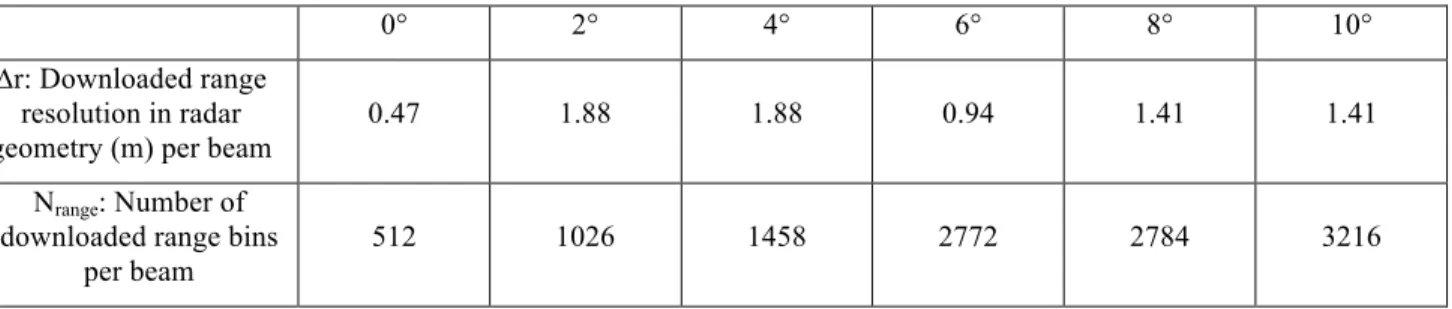
The data downloaded include the power averaged over time (over Nimp samples) and range (over Nrange bins), needed to achieve a range resolution ∆r compatible with the specified minimum detectable wavelength of 70 m (horizontal resolution better than 35 m). The number of range bins (Nrange) determines the footprints in the look direction. Table II lists the values of ∆r and Nrange for each beam. The corresponding footprint dimension (on the Earth's surface) ranges between 25 and 28 km for the beams used for wave spectrum estimation (6°, 8°, 10°). Nimp and the corresponding integration times are provided in Table III.

Table II: Range resolution, number of range gates Nrange used for on-board range integration, and number of range bins in the downloaded

signal.

0° 2° 4° 6° 8° 10°

∆r: Downloaded range resolution in radar geometry (m) per beam

0.47 1.88 1.88 0.94 1.41 1.41

Nrange: Number of downloaded range bins

per beam

512 1026 1458 2772 2784 3216

B. System definition 1) Chronogram

The beams corresponding to the six different elevation angles are illuminated sequentially, within temporal windows having different specific durations (Table III). The time allocated to one single beam measurement is referred to as a “cycle”, whereas the duration of a full sequence

of consecutive beam cycles is referred to as a “macro-cycle”.

The cycle durations have been chosen in such a way as to optimize the number of independent echoes used for the signal integration over time. This is required to reduce the noise (in particular that produced by speckle) and to increase the radiometric resolution.

TABLE III

SWIM CHRONOGRAM.THE PULSE REPETITION FREQUENCY (PRF) IS ADAPTIVE ALONG THE ORBIT.NIMP IS THE CONSTANT NUMBER OF PULSES

TRANSMITTED DURING ONE CYCLE.

0° 2° 4° 6° 8° 10°

Ambiguity rank 18 18 18 18 18 18

Min PRF (Hz) 5093 5079 5079 5065 5037 5023

Max PRF (Hz) 5427 5427 5411 5395 5379 5348

Nimp 264 97 97 156 186 204

Max integration time length (ms) 51,8 19,1 19,1 30,8 36,9 40,6

Min cycle length (ms) 52,0 21,2 21,3 32,3 37,9 41,5

The maximum cycle duration is constrained by the migration of resolution cells resulting from antenna rotation and the satellite's displacement along the ground track [16, 21], even though these migrations are partially compensated by the use of a Chirp Scaling algorithm. In the case of the incidence beams at 2° and 4°, the requirement in terms of radiometric resolution (and hence integration time) are more relaxed than at 6°, 8°, and 10°, because these measurements are used only to complement the normalized radar cross-section information over the full range of incidence angles [0-11°], but not to estimate wave spectra. The durations indicated in Table III result from a trade-off taking all of these constraints into account. The Pulse Repetition Frequency (PRF) is of the order of 5 kHz but takes different values for each incidence beam. It also varies with the distance of the orbit with respect to the Earth’s surface (see Table III). Because of these PRF variations, the cycle duration is adjusted in order to always maintain for each beam, a constant number of time-integrated echoes Nimp.

2) Modes of operation

Different options are possible for SWIM operations, described in the following:

- For the macrocycle mode:

The default mode for the macro-cycle consists in sequentially illuminating all of the beams pointing at each elevation angle {0°, 2°, 4°, 6°, 8°, 10°}. It will be used by default. Alternative macro-cycles can be used such as {0°, 6°, 8°, 10°}, {0°, 8°, 8°}, or {0°, 10°, 10°}. For each case, the cycle durations are maintained to the values presented in Table III for the corresponding incidence.

- The antenna mode:

The antenna feed horns may be rotated (nominal mode) or stopped to a prescribed azimuth direction.

- The time-integration mode:

In the nominal case, integration time is set according to the values shown in Table III. In addition, a specific mode referred to as the “speckle mode” is defined, to provide data that

are used during on-ground post-processing, to estimate the speckle density spectrum in accordance with the method proposed in [19]. In this mode, the on-board integration time is reduced to one-third of its nominal value, allowing three averaged waveforms to be obtained per cycle at any given incidence, with each integration corresponding to Nimp/3 averaged samples. In order to maintain a constant data rate, range averaging is increased by a factor of three in this configuration.

For the SWIM operations, it is possible to choose any combination of these modes (macro-cycle, antenna, time-integration).

In addition to these scientific modes, calibration sequences are interleaved on a daily basis, allowing the instrument gain and the impulse response function to be determined. Appropriate corrections are derived, and applied to the raw data to obtain calibrated backscattering coefficients [29].

C. SWIM instrument performances 1) Geometry and resolution

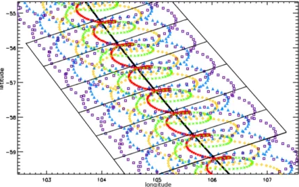
The global swath of the instrument is approximately 90 km left and right of the nadir track. The azimuthal sampling results from the mechanical layout of the feed horns on the rotating plate combined with the illumination sequence of the feed horns. Fig. 4 illustrates the azimuth sampling in the standard operational mode with the six beams illuminated successively. It shows that azimuthal sampling is non-contiguous throughout the macro-cycle. Taking into account the cycle duration, the rotational speed of the horns (5.6 rpm) ensures that at least two observations can be made per 15° azimuthal bin. The surface is illuminated and sampled by the six beams as shown in Fig. 4b: each of the six elevation spot and all azimuths [0-360°] are sampled within the timeframe corresponding to the satellite's along-track displacement of approximately 70 km.

As explained in IV.A.3, the on-board processing is designed to provide an ultimate horizontal resolution, along the line of sight, of 35 m or better. Although the chirp scaling can correct for the effects of the migration along the range axis only (but not for those due to wave front

curvature), simulations were used to check that the effective ground resolution is better than 20 m for all spectrum beams and all range gates (not shown here). This result indicates that the horizontal resolution is compatible with the specified minimum detectable wavelength of 70 m for ocean waves.

Fig. 4 a : Schematic view of the illumination geometry formed by the 6 beams, during 3 macrocyles. One macrocyle comprises the illumination patterns formed by the 6 successively transmitted beams. These are not continuous in azimuth (the black red, green, yellow, cyan and pink footprints are produced

successively).

Fig. 4b: Schematic representation, using geographical coordinates, of a portion of the Earth's surface sampled during approximately 13 macrocycles. The same color code is used as in Fig. 4a : angle of incidence: 0° (black), 2° (red), 4° (green), 6° (yellow), 8° ( cyan), and 10° (pink).

2) Pointing accuracy

The pointing budget of the SWIM instrument has been estimated by taking into account instrument and platform contributions as specified or

measured in the laboratory before launch. These budgets include the accuracy of the mechanical mounting on the platform, the attitude-control system, together with mechanical effects associated with SWIM and the platform (launch,

5.6 rpm 88 km H ~519 km Incidences: 0°-2°-4°-6°-8°-10° Antenna aperture: ~2°x2° 51 9k m

hygrometry, thermoelastic, etc.). The maximum pointing errors estimated at 3 sigma are:

• elevation pointing accuracy < 0.20° (all beams),

• elevation pointing knowledge < 0.08° (all beams),

• azimuthal pointing knowledge < 0.63° (fixed and rotating antenna).

The pointing offset will be also accurately determined from the data processing (ground-processing) by using a best-fit algorithm minimizing with respect to the data, the expected shape of the s0 trend as a function of incidence angle, based on the assumption of geometric optical backscattering, and using the real antenna gain pattern. This algorithm takes advantage of the diversity of the azimuthal pointing directions of the various incidence beams, to retrieve the pointing offset parameters by constraining the trend of s0 as a function of incidence angle. Our numerical simulations, based on this method, show that knowledge of the overall pointing will be accurate to within 0.05°.

3) Radiometry

a) Link Budget

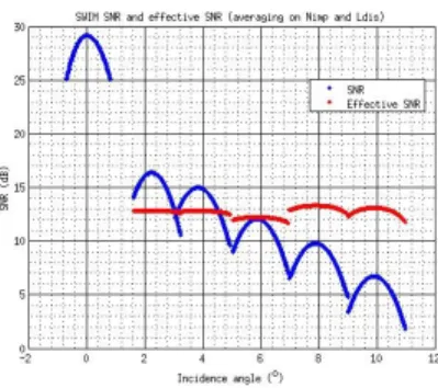
The worst case scenario for the link budget was estimated assuming the lowest values of the normalized radar cross-section, as provided by the TRMM observations [8 dB, 7.4 dB, 6.8 dB, 6.2 dB, 5.6 dB and 5 dB] for the six beams (between 0° and 10°, respectively) and an altitude of 545 km. Figure 5 plots the signal to noise Ratio (SNR) per pulse under these conditions (blue lines). These values correspond to an effective SNR (SNRe) better than 11 dB for any beam (red lines in Fig. 5) corresponding to a radiometric accuracy Kp better than 0.26 dB (Kp=1/SNRe). As Kp can be further reduced by averaging, it becomes negligible at the scale of 0.5° incidence and 15° azimuth bins, which are the scales used for the backscattering coefficient analysis.

Fig. 5 – Link budget of the SWIM instrument for the worst case conditions (see text for details). The SNR is shown by blue lines and the effective SNR (SNRe) is plotted with red lines. The SNRe includes the

on-board averaging over time (Nimp pulses) and over range gates (2 to 4 in

nominal mode, depending on the beam).

b) Normalized radar cross-section

Internal calibration [29] is used to estimate all the radiometric gains and losses and convert signal intensity to normalized radar cross-sections. Analytical and laboratory estimates of the calibration budgets, taking all the internal contributions from the instrument into account show that:

• absolute calibration should be better than ± 0.9 dB (< 0.65 dB for the fixed bias contribution),

• relative calibration error between all beams should be less than ± 0.3 dB.

In order to assess the absolute calibration of the normalized radar cross-section, various additional external, in-flight calibrations will be performed using observations over homogeneous surfaces of known radar cross-sections or at crossing points with other instruments (such as Ku-band altimeters or GPM Ku-band radar). This cross calibration should allow estimating the fixed bias of the error budget. The remaining random error should be below 0.4 dB for each beam.

V. SWIM DATA PROCESSING AND PRODUCTS

A. Overview

The operational near-real time on-ground data processing of SWIM will be carried out in France by the French mission center, CWWIC (CNES Wind and Wave Instrument Center), which will be responsible of producing the following main products in Near-Real-Time (NRT), ie within 3 hours after data acquisition:

- Level 1a: normalized radar cross-section in the radar geometry

- Level 1b: for each SWIM look direction and the beams at 6°, 8°, 10° incidence: radar cross-section modulations, and associated spectral density, impulse response function and speckle

- Level 2:

• for the beams at 6°, 8°, 10°: two-dimensional wave height spectra and their associated parameters

• for the nadir beam: significant wave height and wind speed estimation • for all beams: mean radar

cross-section profiles as a function of incidence and azimuth

A second data center implemented at Ifremer (Institut français de recherche pour l'exploitation de la mer) in France will provide, without the NRT constraints, complementary L2 products as well as L3 and L4 products. In this paper we focus on the CWWIC products whose processing chain is currently being developed and tested, using simulated data as described in the following.

B. Product simulations

1) Nadir products

The performance of the significant wave height and wind speed estimations, derived from the nadir beam, were evaluated using the same approach as for standard altimeter missions (echo simulation and re-tracking algorithm, see [30]). We have implemented simulations (not shown here), showing that the performance is compliant with the requirements, and similar to that of the most recent altimeter (Hs within 10% or 0.5 meters, whichever is greater, rms error on wind speed less than 2 m/s).

2) Off-nadir products

An end-to-end instrument software simulator, SimuSWIM, has been developed, to validate the design of the instrument and prepare the processing algorithms. This is an updated and extended version of the simulator previously developed by [21], for the purposes of dimensioning the initial version of the system. The simulator includes a direct simulation module

(from the surface to the instrument signal) and an inversion module, based on the ground segment prototype, including all of the steps to be used for the inversion of real products, when they become available.

The direct module simulates the radar signal backscattered from the sea surface described by its two-dimensional field of elevation and slopes. The surface topography can be generated numerically, using either a predefined wave spectrum prescribed by an empirical formulation, the output from a wave forecast model, or data taken from in situ measurements. The instrument's characteristics and geometry are taken into account, and the beam footprints and range gates are computed on the sea surface. For the six beams, the mean backscattered power is

computed using a Geometrical Optics

backscattering model ([22]) and a Gaussian probability density function to represent the wave slopes, with the mean square slope having an empirical dependence on wind speed [31]. The signal modulations produced by long waves are then simulated using Eq. (5, 6), the sea surface topography and radar propagation. The simulated radar echoes include the effects of perturbations introduced by speckle and thermal noise. The on-board processing steps are also simulated (migrations, on-board averaging over the cycle, and gain and range loops).

The different steps implemented by the inversion module and their outputs are described in sections V-C to V-E below, for each product. The inversion module makes use of prototypes of the future ground segment algorithms.

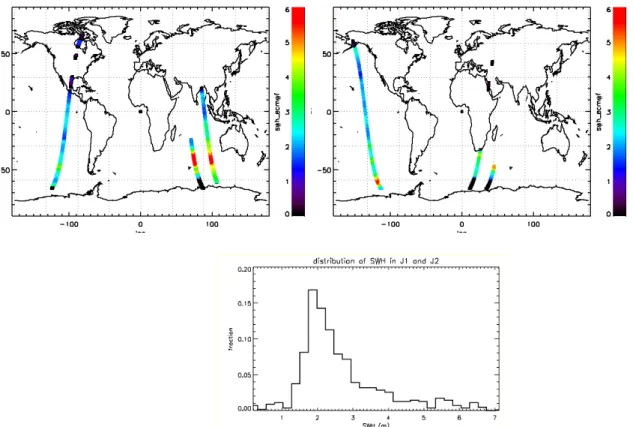
The test set presented in this paper makes use of the directional spectra of ocean waves, provided by hindcasts from the WAM wave model used at ECMWF [32]. Simulations were carried out over two complete CFOSAT orbits (105 minutes per orbit). The first of these (J1) passes over very high wind and waves in the South Indian ocean, which are representative of high sea states (up to 6-7 m). The second orbit (J2) is more representative of the conditions encountered

under conditions of moderate wind and waves (generally around 2-3 m, with a maximum of 5 m). The distribution of significant wave heights encountered along these orbits is shown in Fig. 6.

The datasets from these simulations are available on-line:

http://www.aviso.altimetry.fr/fr/missions/mission s-futures/cfosat/access-to-simulated-data.html

Figure 6: Significant wave height provided by the ECMWF along the selected orbits for the J1 (top left) and J2 (top right) simulation. The histogram of Hs

corresponding to the combined analysis of the J1 and J2 simulations is shown on the bottom plot.

C. L1A processing

The level 1a (L1a) processing provides calibrated radar echoes from the six beams (normalized radar cross-section in the radar geometry), and the associated localization of each range gate (coordinates with respect to ground track and geographical North).

This processing requires the use of calibration parameters, which are provided independently by calibration sequences. These will be updated on a daily basis.

The main steps of L1a processing are:

• correcting the mean level of thermal noise, • normalizing the received power,

• computing the geometry for each gate (range distance, ground distance from

nadir point, elevation, incidence, latitude and longitude),

• computing the integrated antenna gain in the acquisition geometry,

• inversion of the radar equation.

Fig. 7a and 7b provide examples of simulated L0 and L1a products.

Figure 7a. Example of the L0 output power for each of the six beams during one cycle. At this processing step, no compensation of the

Figure 7b. Example of the L1a output for the normalized radar cross-section, plotted for a single macro-cycle as a function of elevation angle.

D. L1b processing

The level 1b (L1b) processing provides intermediate products that are specific of the spectrum beams (6°, 8°, 10°) measurements over ocean surface.

The successive steps applied during L1b processing are:

- calculating the mean value and mean trend of s0, using a polynomial fit,

- calculating the relative fluctuations ds0(r) around the mean trend, as a function of radial distance (Eq.4),

- re-sampling the signal fluctuations, in order to compute their value in the surface reference frame ds0 (x),

- calculating the fluctuation spectrum (Eq. 12),

- calculating the modulation spectrum, and applying corrections for the impulse response function and the speckle density spectra (Eq .11).

By default, the impulse response (IR) is assumed to be that defined in the parametric model proposed by [16, 17], which assumes a Gaussian shape for its density spectrum (Eq. 13, 14). In addition, since the impulse response function is obtained from the calibration sequences, it will also be possible to make use of the measured IR, rather than that provided by the model. Our simulations show that under nominal conditions, the parametric model is sufficiently accurate.

The speckle spectral density is estimated from Eq. (15), i.e. assuming it to be inversely proportional to the number of independent samples averaged in the radar echo at Level 1a. As the simulations cannot take all aspects of the speckle noise into account (in particular the correlation time of the scatterers, which may dominate the Doppler bandwidth effect under certain geometrical or sea state conditions), we also plan to use alternative methods to estimate the density spectrum of speckle, and will test these methods in detail during the commissioning phase. These alternative methods are based on: i) the noise floor of the signal fluctuation sepctrum ii) estimations from “cross-spectrum” analysis [10] applied to the data acquired in special modes (macro-cycles 0-8-8 or 0-10-10 with reduced time integration); and iii) the “speckle mode” of the time-integration mode, as proposed in [18].

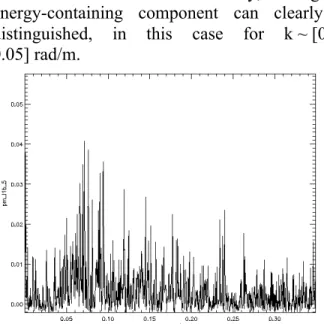
Fig. 8 shows one sample of a spectral density of signal in the direction of wave propagation. It shows that at this level of processing, the spectral modulations remain somewhat noisy, although the energy-containing component can clearly be distinguished, in this case for k ~ [0.02-0.05] rad/m.

Figure 8: Spectral density of signal modulations, expressed as a function of wave number (rad/m).

E. L2 processing

The level 2 (L2) processing provides L2 products, which refer to geophysical data representative of

geographic boxes with dimensions of approximately 70 x 90 km, as shown in Fig 4b. These dimensions allow directional wave spectra to be computed over 180° wave propagation directions, using the concatenation and fusion of radial spectra derived from a single beam (6°, 8° or 10°), or from the combination of three beams (6°, 8°, and 10°).

The L2 products are obtained by processing the L1a and L1b products, as described in the following:

- averaging of the s0 values, over bins defined by intervals of 0.5° in incidence, and 15° in azimuth,

- averaging of the modulation spectrum in 15° azimuthal intervals, and 65 wavenumber bins dk, which fulfill the relationship dk/k = 0.1

- application of the tilt modulation transfer function (MTF) to the modulation spectrum, to estimate the wave slope spectra k2E (Eq. 7-8),

- application of a partitioning algorithm to detect up to three wave components in the 2D polar spectrum; the partitioning algorithm is based on the detection of the spectral maxima, and the use of watershed detection, as proposed in [33]. The latter method has been adapted (noise reduction, discretization of energy levels, and iterative scheme) in order to cope with the noisy nature of the 2D spectra [34].

- calculation of the main parameters in the 2D spectrum, and its partitioning (total energy, peak direction, peak wavelength). In this step, the modulation spectra obtained from L1b are converted to wave spectra, using (Eq.7), which requires an estimation of the parameter <a>. By default (method called MTF1), <a> is calculated from Eq. 8, in which the term ∂(lns0/∂q is estimated from the observations themselves. This estimation is very sensitive to the accuracy of the mean trend of s0 as a function of incidence (i.e. very sensitive to the accuracies of the pointing knowledge and relative calibration between the 6 beams), and requires data over a

range of incidence angles greater than that covered by each individual beam. Although the finally obtained accuracies of the values of the relative s0 and mispointing knowledge (following on-ground processing estimations) are compatible with an accurate estimation of ∂(lns0)/∂q , we also plan to implement two alternative methods. These will be applied when the non-standard macro-cycle mode is selected (acquisition on beams at 2° and 4° not activated). The first of these, referred to as MTF2A, is based on the use of Eq. 8, but with ¶s0/∂q being estimated from an empirical model. This model is established from the existing Ku-Band radar data sets, and is currently based on results presented in [23], derived from the TRMM-Precipitation radar, tabulated in terms of wind speed and significant wave height. Using the wind speed and significant wave height provided by the nadir beam, or derived from ancillary data from meteorological models, the alternative tilt MTF will be estimated from these look-up tables. The third method (referred to as MTF2B) is based on the assumption that the normalized radar cross-section can be described by the geometrical optics backscattering [22]. Under these assumptions, Eq. (8) becomes: 𝛼 = _G%& H 𝑐𝑜𝑡𝜃 − 4 𝑡𝑎𝑛𝜃 − $ no/:_S Npq (_ rsPS ) NrsPS % (16) where p(tanq) is the wave slope probability density function (pdf) in the radar look direction. By assuming the slope pdf to be an isotropic Gaussian function, whose variance (mean square slope) is related to the wind speed, <a> can be estimated as: 𝛼 = _G%& H 𝑐𝑜𝑡𝜃 − 4 𝑡𝑎𝑛𝜃 − 2 rsPS) C//(u) % (17) where mss(U) = AmssU + Bmss with Amss = 0.0016 and Bmss = 0.016 as proposed in [31].

To summarize, for each value of incidence (6°, 8°, 10°), the L2 products for each box will include:

- the wave slope directional spectra for 65 wavenumber intervals and 12 azimuthal intervals

in the range between 0° and 180°, with an 180° ambiguity in the direction of propagation,

- the mean modulation transfer function,

-the omni-directional wave slope spectrum, the confidence intervals per wavenumber bin, and the significant wave height,

- the detected partition mask, which is used for partitioning of the 2D polar spectrum into as many as three partitions, characterizing different wave components (swell, wind sea),

- the characteristic parameters of the directional wave spectrum and its partitions (dominant direction, dominant wavelength, significant wave height).

In addition, for the same geolocalized boxes, the L2 products will contain the mean s0 values, as a function of incidence and azimuth.

Finally, the products produced by processing of the nadir data will be merged with the L2 products (significant wave height, normalized radar cross-section and wind speed).

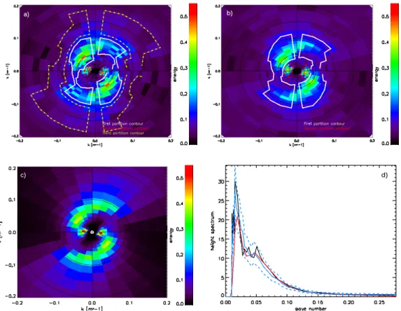
Fig. 9 illustrates the performance of the L2 product retrieval, for a wave spectrum sample chosen characterized by mixed sea conditions (wind sea and swell). It shows that the 2D wave spectrum obtained from the 10° beam observations (Fig. 9a) as well as that obtained by merging the 6°, 8°, and 10° beam observations, is quite consistent with the reference shown in Fig. 9c (the ECMWF spectrum used as input for the simulation): the two main wave components of the spectra are retrieved, with a swell component (dashed red contours) and a wind sea component (continuous white contours), with direction and peak wavenumbers very similar to those found in the reference spectrum (Fig. 9c). The spectrum obtained by merging the 6°, 8°, 10° inversions shows less spectral fluctuations (less noise in the estimation), thanks to the greater number of degrees of freedom in this case. The noise present in the case of a single spectral measurement (10° incidence) leads to the detection of a third wave component, visible in Fig. 9a (yellow dashed

contours), which is likely an artifact. The corresponding omni-directional wave height spectra are plotted in Fig. 9d, showing that the inverted spectra (black and blue lines) are in good qualitative agreement with the reference spectrum (red line). As in the case of the 2D representations, the spectral fluctuations (noise) are reduced when the inversions computed at 6°, 8° and 10° are combined. When homogeneous conditions are fulfilled at the scale of the 3 combined measurements (70 x 90 km), it may be advantageous to use the combined incidence product. In other situations, although the results may be a little noisy, it may be advantageous to interpret the data for individual values of incidence.

In order to quantify the overall accuracy of the L2 products, we used the J1 and J2 test sets to simulate the radar signal and inverted products, over two complete orbits. In both cases, prototype ground segment software was used. The mean errors are computed for each partition rank, as:

• Δ𝐸 =w*w?xy

w?xy , (18a) • Δ𝑘 =,z*,z_?xy

,z_?xy , (18b) • Δ𝜙 = 𝜙_{_}− 𝜙_{__;|}} (18c)

where the variables 𝐸, 𝑘_, 𝜙_, refer respectively

to the total energy, dominant wavenumber and dominant direction in the inverted wave spectra partitions, and the same quantities with the subscript ref refer to their counterparts derived from the reference spectra (WAM hindcast). The dominant wave number and directions are estimated as the energy-weighted mean wavenumber and direction over a region close to the peak of each partition delimited by 2/3 of the maximum energy.

Figure 9: (a) Example of a directional wave spectrum retrieved using the inversion algorithm and simulation tool, for the case of the 10° incidence beam. The spectral density is shown in color, the wave number scale is indicated on the horizontal

and vertical axis, and the wave propagation direction is given by the angle from the top of the figure (with a 180° ambiguity). The contour lines (dashed red, continuous white, and dashed yellow) show the contours of the three detected

partitions. This example corresponds to a situation with mixed sea conditions, characterized by a total significant wave height of 4 m. (b) same conditions as for (a), computed from the average of the three spectra, determined at incidence angles

of 6, 8, and 10°. (c) Reference directional wave spectrum derived from the ECMWF model. (d) Omni-wave height directional spectrum corresponding to the 2D spectra shown in (a) (black line) and (b) (blue line). The dashed lines correspond to the 95% confidence interval, and the red line corresponds to the reference spectrum used as input for the

simulation. The total energy of each partition is estimated as:

𝐸 = 4•8€𝐹(𝑘, 𝜙)

4••‚ 𝑘𝑑𝑘𝑑𝜙

,•8€

,••‚ (18d)

where kmin, kmax , Fmin, Fmax delimit the

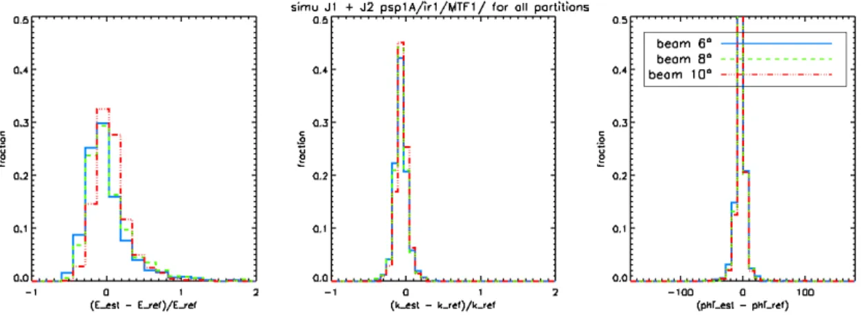
partition.The results obtained for all partitions using the J1 and J2 datasets are shown in Figs. 10. Fig. 11a-b shows the results for each of the first two partitions. Figs.10 and 11 show that the peak

wavenumbers and directions are globally well retrieved for all partitions, and all incidence configurations (6°, 8°, 10°), with accuracies in agreement with the specifications (10% in wavelength, 15° in azimuth). As for the energy of the wave partitions, Fig. 11 indicates good performance, except for small values of Hs (< 1.5 m), for which the computed energy is offset by a bias with respect to the reference.

Figure 10: Normalized energy, peak wave number and peak direction error histograms for each detected partition in the 2D wave spectra, for the J1 and J2 simulation sets.

Table IV lists the mean errors, the scatter index (or standard deviation for the peak direction) computed with respect to the reference values, for all partitions having a significant wave height greater than 2 m. The energy estimations in each partition achieve the expected performance. The best energy estimation is obtained with the beam at 10°, because the signal-to-noise ratio is always higher at this incidence than at 6° or 8°. Following the launch of CFOSAT, it is planned to correct the biases observed in the smallest energy partitions (< 1.5 m), using real data to provide external reference values.

The same error analysis was also carried out as a function of wind speed (not shown), confirming the absence (under all wind conditions) of any bias for the peak wavenumber and direction, and showing that the errors in the estimation of wave energy had no significant dependence on wind speed. This type of analysis will be repeated with

larger simulated datasets, prior to the launch of CFOSAT. Similar, detailed analyses will also be carried out during the calibration/validation (CAL/VAL) phase. The assessment of energy retrieval performance will be particularly important, for the selection of the parameter <a>, which governs the modulation transfer function. The speckle model may also require various adjustments, after launch.

Table IV: Mean relative bias and scatter index for the energy and peak wavenumbers, and mean absolute bias and standard deviation for the peak directions of partitions when

Hs > 2 m. The 3 columns on the right refer to results for the 6°, 8°, and 10° beam, respectively

Figure 11: Relative difference in energy (top), wavenumber (middle), and absolute difference in direction (bottom), as a function of the reference significant wave height (SWH), obtained for the first partitions (left-hand column) and the second

partitions (right-hand column), using the J1 and J2 simulation sets.

VI. CONCLUSION

In this paper we present the SWIM Ku-Band radar instrument, designed and developed for the future CFOSAT Chinese-French oceanographic mission. SWIM is a new type of space-borne scatterometer, developed for the measurement of the directional spectra of ocean waves, using a concept designed to overcome the limitations encountered with SAR systems.

This instrument is based on a real-aperture, conical scanning fan-beam system inspired by the pioneering work described in [16,17], and by the results obtained from the airborne systems described in [18, 20]. This technique interprets modulations of the observed radar cross-section in the range direction, to determine the local slopes of long ocean waves. A description is provided of the scientific requirements for the geophysical products, together with the ensuing performance specifications of the instrument.

The inversion algorithms are also presented in detail, and the results of an end-to-end simulator, applied to synthetic data representative of ocean wave fields over two orbits, are discussed. This shows that, when associated with the predicted performance of the instrument, the proposed inversion methods are fully compliant with the scientific requirements on the directional wave spectra and their associated parameters: ocean waves in the [70m, 500m] range to be measured with an accuracy better than 10% in wavelength, 15° in direction, and 10% in significant wave height (or 20% in energy), for all wave systems with a significant wave height greater than approximately 1.5 m. In addition, the system will provide the scientific community with the mean profiles of the normalized radar cross-sections at near-nadir incidence angles [0-10°], as well as the significant wave heights and wind speeds measured by the nadir beam.