EcoGRAFI
2nd International Conference on Bio-based Building Materials &
1st Conference on ECOlogical valorisation of GRAnular and FIbrous materials
June 21th - 23th 2017 Clermont-Ferrand, France
THERMAL INSULATION MATERIALS FROM RENEWABLE RESOURCES:
THERMAL AND HYGRIC PERFORMANCES
M. Viel*, F. Collet, C. Lanos
Université Rennes 1, Laboratoire Génie Civil et Génie Mécanique, Rennes, France * Corresponding author: marie.viel@univ-rennes1.fr
Abstract
The European ISOBIO project aims to develop new bio-based building insulating materials which contribute to reduce environmental impacts of buildings. The developed materials shall have low embodied energy and low carbon footprint and shall contribute to reduce energy needs of buildings ant to ensure high hygrothermal comfort of users. This study investigates the valuation of agro-resources as bio-based aggregates and as binding material to produce wholly bio-based composites. Two types of aggregates: hemp shiv and corn cob residues (obtained after alkali treatment on the corn cob), and five types of green binders are investigated. Specimens are produced to characterize thermal and hygric properties of developed composites and to identify the best mixture between aggregate and binder. They show interesting thermal and hygric properties. They have low thermal conductivity ranging from 0.067 to 0.148 W/(m.K) and depending on the mix (aggregate with binder). They are excellent hygric regulators (MBV >2 g/(m².%RH)). These results suggest that developed composites can be used as building materials but not for the same types of use. In fact, some composites would be more suitable for thermal insulating products and others would be better suited to indoor facing panels.
Keywords:
Agricultural waste valuation, Thermal insulation materials, Bio-based composites, Hemp shiv, Corn cob, Green binders, Moisture Buffer Value, Thermal conductivity
1 INTRODUCTION
This study is part of the European ISOBIO project which aims to develop new bio-based building insulating materials. The aim is to reduce the embodied energy of materials while also reducing the total energy needs of buildings and allowing high hydrothermal comfort of users. Two kinds of products are developed within ISOBIO project: insulating panels and bio-based insulating composites to be implemented on-site. The project focuses on the valuation of agro-resources as bio-based aggregates and as binding material to produce wholly bio-based composites. Five agro-resources are considered in ISOBIO project: hemp, flax, rape, wheat and corn cob. They are available as straw, shiv, fibre or dust.
For compressed straw panels, no additional binder is needed to provide a minimum of cohesion. The raw material is just cleaned and compressed between two hot plates where it undergoes a hydrothermal treatment at 200°C (as the STRAMIT Process [Glassco 1987]). The cohesion of the obtained material is then ensured by the released lignin (between 8 and 17%), hemicellulose (between 28 and 33%) and cellulose (between 33 and 42%) from the wheat straw [Sun 2000]. Based on this observation, it is possible to use the components contained in the bio-based aggregates to formulate a green binder. Initial work was done to evaluate the ability of hemp shiv to be bonded by wheat straw using the same
compression process. Hemp shiv was mixed with wheat straw chopped with a lab blender to obtain bio-based composites. Several compositions were tested; it was shown that wheat straw allowed a good cohesion of the composite when the dry mix included at least 15% of wheat straw [Collet 2016].
This study investigates the development of bio-based composites to be used to produce insulating panels. Two types of aggregates: hemp shiv and corn cob residues (obtained after alkali treatment on the corn cob) for its good hygric property, are considered. Then, six green binders are used to be compared. Two bio-binders are obtained by extraction process on corn cob and on flax fine. Others come from industry as black liquor (by-product of paper industry), molasses (by-product of sugar industry), commercial lignin (by-product of wood industry) and the PLA (thermoplastic binder from renewable resources). Specimens are produced to qualify the hygrothermal performances of developed composites. The aim of these characterizations, in link with the objectives in term of reduction of energy needs of buildings and in term of hygrothermal comfort of users, is to identify the best mixture between aggregates and binder.
2 MATERIALS AND METHODS
2.1 Raw materials Binders
Six types of binders are considered in this study.
Two bio-binders are developed from agro waste valuation, and four are available from industrial waste valuation. Considering the previous study [Collet 2016], the developed bio-binder by extraction of soluble content. This method is first studied for wheat straw. The extraction process consists in infusing wheat straw in solvent for several hours. Then, wheat straw is pressed in order to collect all solvent. This solvent is partially evaporated in order to control the concentration of the solution (Fig. 34).
Fig. 34: The extraction process on bio-aggregates
Several trials are achieved to identify the optimum conditions. Indeed, for the extraction process, many factors can affect the yield:
▪ The maceration time, ▪ The grain size, ▪ The nature of solvent, ▪ The solvent concentration.
Following those observations, the optimum conditions identified with a yield of 50 % were maceration in alkali solvent during 4 hours at 90°C.
This process is then applied for each raw material supplied by CAVAC, industrial partner of ISOBIO project (these materials are presented in other conference paper [Viel 2017]) and two raw materials are identified as the best for this use. These ones are corn cob and flax fines. Three other binders are bio-binders from industry as black liquor (waste of paper industry), molasses (by-product of sugar industry) and commercial lignin (by-product of wood industry, Biochoice® powder).
The last binder is a biodegradable thermoplastic from renewable resources: the Poly-Lactic Acid (PLA provided by Galactic - Belgium). This polymer is characterized by very high mechanical properties (flexural strength of 17.8 MPa and compression strength higher than 50 MPa, elastic modulus of 3500 MPa) and glass transition temperature around 180°C. PLA is marketed in granular form. To be used, it is reduced in chips.
All the binders are presented Fig.2.
Fig. 35: Binders used to tested composites formulation Aggregates
Two types of aggregates are considered in this study (Fig.
36).
The shiv is a commercial product (Biofibat – CAVAC, France) commonly used to produce hemp concrete. Its bulk density is about 100 to 110 kg/m3. The mean width of particles (W50) is 2.2 mm and the mean length (L50) is 8 mm. The maximal width is 5 mm and the maximal length is 19 mm.
The corn cob is the support for maize grains and maize cultivation’s by-product. Its bulk density is about 390 kg/m3. The mean width of particles is 3.78 mm and the mean length is 5.15 mm. The maximal width is 4.77 mm and the maximal length is 6.47 mm. This aggregate is used to make a green binder with their soluble content in the alkali solvent and the corn cob residues obtained is used as aggregates in the composites formulation. After the extraction, the bulk density of the corn cob residues is about 365 kg/m3.
Fig. 36: Aggregates used to tested composites formulation 2.2 Composites
Design of Experiment (DOE)
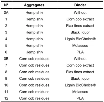
For this study, two types of aggregates and six types of binders are tested. To get a large number of information, screening design is used and more specify Hadamard matrix. This experience design will allow understanding the effects of factors on the composites properties (thermal conductivity and moisture buffer value) [Rabier 2007]. Tab. 34 shows the established experience design. One factor has 2 levels for aggregates (hemp shiv or corn cob residues), and one other factor has 7 levels, for binders (without binder, corn cob extract, flax fines extract, black liquor, lignin BioChoice®, Molasses or PLA).
Tab. 34: Formulation of composites
N° Aggregates Binder
0A Hemp shiv Without
1 Hemp shiv Corn cob extract
2 Hemp shiv Flax fines extract
3 Hemp shiv Black liquor
4 Hemp shiv Lignin BioChoice®
5 Hemp shiv Molasses
6 Hemp shiv PLA
0B Corn cob residues Without
7 Corn cob residues Corn cob extract
8 Corn cob residues Flax fines extract
9 Corn cob residues Black liquor
10 Corn cob residues Lignin BioChoice®
11 Corn cob residues Molasses
12 Corn cob residues PLA
Then, this experimental design is converted in experiment matrix, which is a mathematical entity. It includes as many lines (noted n) as formulations and as many columns (noted p) as unknown coefficients in the model. This
experimental design can be rewritten in the form of the following equation:
{𝒀} = {𝑩} (𝑿) + {𝒆} (1)
with:
▪ {Y}: response vector, ▪ (X): matrix of the model, ▪ {B}: coefficient vector, ▪ {e}: vector of the gaps.
The mathematical analysis allows estimating the coefficients {B} and the residues {e} by the least squares method. The effects of the factors on the responses are calculated as:
{𝑩} = ( 𝑿𝑿𝒕 )−𝟏( 𝑿𝒕 ){𝒀} (2)
where (tXX)-1 is a dispersion matrix and (tX) is the transpose of the matrix. Once the Bi coefficients are determined, they are used in the following equation to predict the responses yi.
𝑦𝑖= 𝐵0+ 𝐵1. 𝑥1,𝑗+ 𝐵2. 𝑥2,𝑗+ 𝐵3. 𝑥3,𝑗+ 𝐵4. 𝑥4,𝑗+ 𝐵5. 𝑥5,𝑗+ 𝐵6. 𝑥6,𝑗 + 𝐵7. 𝑥7,𝑗+ ∆ + 𝜀 (3) with:
▪ yi: response, ▪ xi, j: level of the factor
▪ B0: theoretical average value of the response (constant),
▪ Bi: effect of the factor, ▪ ∆: the lack of fit, ▪ ε: random error.
The robustness of the defined model is tested with two tools: F-test for the significance of the model and the t-test for significance of the coefficients (Fig. 37).
Fig. 37 : Flow chart of statistical analysis for defining the robustness of the model
The analysis of variance (ANOVA) studies the differences of average between the experimental and theoretical responses. It determines if the defined model is significant or not. The total variation in Y (total sum of squares, SSTO) is divided into two components: the one is the equation regression component (regression sum of squares, SSR) and the other is the residual component (error sum of squares, SSE). The first is tested in comparison with the second. These components are sum of the squared deviations and their equations are summarized in the following analysis of variance table (Tab. 35).
Tab. 35: Standard analysis of variance table Source of variation Degrees of freedom Sum of
squares Mean square F*
Regression 𝑝 𝑆𝑆𝑅 𝑀𝑆𝑅 = 𝑆𝑆𝑅𝑝 𝐹∗= 𝑀𝑆𝑅 𝑀𝑆𝐸 Residual error 𝑛 − 𝑝 − 1 𝑆𝑆𝐸 𝑀𝑆𝐸 = 𝑆𝑆𝐸 𝑛 − 𝑝 − 1 Total 𝑛 − 1 𝑆𝑆𝑇𝑂 with: ▪ 𝑆𝑆𝑅 = ∑(𝑦𝑖− 𝑦̂𝑖)², ▪ 𝑆𝑆𝐸 = ∑(𝑦̂𝑖− 𝑦̅)², 𝑖 ▪ 𝑆𝑆𝑇𝑂 = 𝑆𝑆𝑅 + 𝑆𝑆𝐸.
where 𝑦𝑖 are the experimental responses, 𝑦̂ are the theoretical responses and 𝑦 is the mean response. Then the F* ratio is compared to a critical variable taken in F-table for α = 5% (risk). Thus, if F* is higher than the considered critical level, the model is considered to be statistically significant.
Another statistical analysis is performed on the coefficients.
Tab. 36: Table of statistical analysis of the coefficients
Coefficient σ texp Significance
Bi 𝜎𝑖= √𝑀𝑆𝐸 × 𝑐𝑖𝑖 𝑡𝑒𝑥𝑝,𝑖= 𝐵𝑖
𝜎𝑖 texp > tth
with:
▪ σi: standard deviation of Bi,
▪ cii: diagonal term of the level i of the (tXX)-1 dispersion matrix.
Then the texp is compared to a critical variable from the t-distribution for α = 5% (risk). Thus, if texp is higher than tth, the factor effect is considered to be statistically significant. If a coefficient is considered not relevant, it is possible to eliminate it but its impact on the adjusted determination coefficient ra² will need to be evaluated.
In the presence of several variables, the determination coefficient r² must not be used to compare the descriptive quality of the different models. The use of determination coefficient adjusted ra² is required. This coefficient takes into account the number of variables present in the model and it depends on the following equation:
𝒓𝒂𝟐 = 𝒓𝟐 × 𝒏−𝟏𝑫𝑭 = 𝟏 − 𝒔𝒖𝒎 (𝒚,𝒊
𝟐)
(𝒏−𝟏)×𝒗𝒂𝒓 (𝒚𝒊) ×
𝒏−𝟏
𝒏−𝒑−𝟏 (4)
More the ra² is close to 1, more the calculated values will be close to experimental values [Goupy 2006; Oehlert 2000].
Composites production process
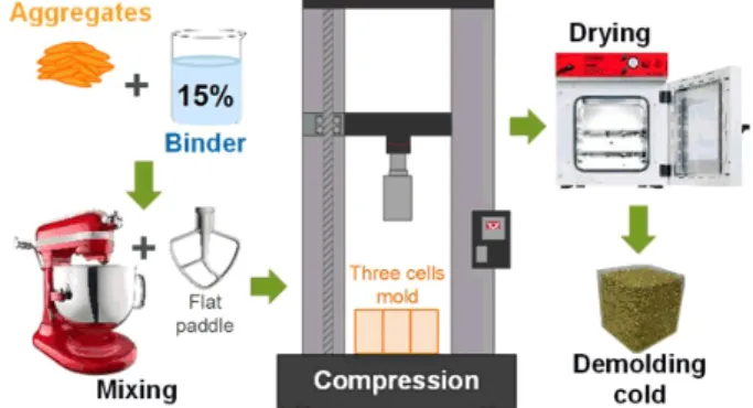
The bio-aggregates are moistened with the binder into water (except for PLA). To ensure a good cohesion, a content of 15% of dry binder is used. Three composites are produced from the same mixture. This mix is divided into three equal parts (A, B and C) and each part is introduced in one of three cell of the mold. After, each part is compacted 5 times at 0.25 MPa in the mold, which is then placed in an oven at 190°C for 2 hours. The three composites of dimensions 100 x 100 x 100 mm3 are demolded cold (Fig. 38).
Fig. 39 shows the produced composites. The composites
n°11 and n°12 have not been produced due to the bad cohesion between the binders (molasses and PLA) and the aggregates (corn cob residues).
Except for the composite n°6, the composites based on hemp shiv have very close densities ranging from 177 to 191 kg.m3. The composite based on hemp shiv and PLA (n°6) has the highest density (273 kg/m3) of the composites based on hemp shiv. The composites based on corn cob residues have a density much higher than composites based on hemp shiv, due to much higher density of aggregates. The three composites, with the aggregates extracts and black liquor, have very close densities ranging from 520 to 557 kg/m3. The composite with the lignin has the lowest density (457 kg/m3) of the composites based on corn cob residues.
Fig. 39: Developed composites Tab. 37: Apparent density of composites
N° 1 2 3 4 5 Density (kg/m3) 177.69 ± 2.37 179.65 ± 5.68 191.42 ± 0.90 179.04 ± 1.26 187.36 ± 1.38 CoV 1.33% 3.43% 4.44% 2.80% 1.95% N° 6 7 8 9 10 Density (kg/m3) 272.89 ± 18.95 519.86 ± 9.80 556.94 ± 9.69 526.98 ± 5.38 457.26 ± 0.93 CoV 4.01% 1.67% 1.19% 3.61% 1.21% 2.3 Characterization methods Thermal characterization
The thermal characterization is based on the measurement of thermal conductivity after drying at 60°C and cooling to ambient temperature in desiccators with silica gel. The measurement is performed in a desiccator and with a transient method: Hot Wire. This method is based on the analysis of the temperature rise versus heating time.
∆𝑻 = 𝟒.𝝅.𝝀𝒒 (𝒍𝒏(𝒕) + 𝑪) (5)
Where ∆T (°C) is the temperature rise, q (W/m) is the heat flow per meter, (W/(m/K)) is the thermal conductivity, t (s) is the heating time and C is a constant including the thermal diffusivity of the material.
The measurement is performed with the sensor sandwiched between two specimens. In order to prevent the presence of an air gap, a weight is put on the specimens. The heat flow and heating time are chosen to reach high enough temperature rise (>10°C) and high correlation coefficient (R²) between experimental data and fitting curve. In this study, the commercial CT Meter device is equipped with five centimeters-long hot wire. The power used is 142 mW (n°1 to 4) or 205 mW (n°5 to 10) and the heating time is 120 seconds. These settings allow meeting the previous requirements (temperature increase higher
than 10°C and high R² value). According to the manufacturer, the expected accuracy is thus better than 5%. For each formulation, three pairs of specimen are considered by combining differently the three specimens (A&B, C&B and A&C, Fig. 7). The thermal conductivity of a pair of specimens is the average of three values with a coefficient of variation (ratio of the standard deviation to the average value) lower than 5%. The thermal conductivity of a formulation is the average of the nine values from the three pairs of specimens.
Fig. 40: Thermal conductivity measurement Hygric characterization
The hygric characterization is based on the measurement of the moisture buffer value (MBV) of materials, which characterizes their ability to moderate the variations of indoor relative humidity in buildings.
The moisture buffer value is measured following the Nordtest protocol [Rode 2005]. Specimen are sealed on all but one surfaces. After stabilization at 23°C, 50% RH, specimens are exposed to daily cyclic variation of ambient relative humidity (8 hours at 75% RH and 16 hours at 33% RH) in a climate chamber (Vötsch VC4060, Fig. 41).
Fig. 41: Experimental device for the measurement of Moisture Buffer Value
The moisture buffer value is then calculated from their moisture uptake and release with:
𝑴𝑩𝑽 = 𝑨.(𝑹𝑯 ∆𝒎
𝒉𝒊𝒈𝒉−𝑹𝑯𝒍𝒐𝒘) (6)
Where MBV (g/(m².%RH)) is the moisture buffer value, ∆m (g) is the moisture uptake/release during the period, A (m²)
is the open surface area and RHhigh/low (%) is the high/low relative humidity.
Temperature and relative humidity are measured continuously with sensor SHT75 and with sensor of the climatic chamber; the air velocity in the surroundings of the specimen ranges from 0.1 to 0.4 m/s for horizontal velocity and is lower than 0.15 m/s for vertical one.The specimens are weighed out of the climatic chamber five times during absorption period and two times during desorption one. The readability of the balance is 0.01 g and its linearity is 0.01 g. The accuracy of the moisture buffer value is thus about 5%. For each formulation, the MBV is measured on the three specimens and the MBV of the formulation is the average value of the three specimens.
3 RESULTS
3.1 Thermal characterization
To validate thermal conductivity measurement, an infrared thermography picture a photo is taken on each specimen immediately after measurement. For all specimens, all the probe volume is in the specimen, as shown as examples on Fig. 42 for formulations 5 (left) and 8 (right) for which heating power is respectively 142 mW and 205 mW . Thus, the measurements are validated.
Fig. 42: Infrared thermography pictures of specimens 5 (on the left) and 8 (on the right) immediately after the
thermal conductivity measurement
Tab. 38 and Fig. 43 give the average value, the standard
deviation and the coefficient of variation of thermal conductivity of studied composites.For all tests, the correlation coefficient between experimental data and fitting curve is very close to one, higher than 0.9996. More, for each composite, experimental values are very close to each other. The coefficient of variation is lower than 4% between the nine measurements (three pairs and three measurements by pair). This induces great confidence in thermal conductivity values.
Tab. 38: Thermal conductivity of composites N° λ (W/(m.K)) σ (W/(m/K)) CoV (%) 1 0.0708 0.0009 1.22 2 0.0702 0.0012 1.75 3 0.0711 0.0015 2.05 4 0.0675 0.0013 1.88 5 0.0704 0.0008 1.18 6 0.0786 0.0017 2.18 7 0.1403 0.0041 2.92 8 0.1479 0.0047 3.20 9 0.1365 0.0048 3.55 10 0.1284 0.0047 3.66
The thermal conductivities of developed composites, at dry state, range from 0.0675 to 0.1479 W.m-1.K-1. The composites made from hemp shiv as aggregates, have the lowest thermal conductivity (between 0.0675 and 0.0786 W.m-1.K-1). The composite with the PLA has a thermal conductivity slightly higher than the others made with the hemp shiv. The composites made from corn cob residues as aggregates, have the highest ones (between 0.1284 and 0.1479 W.m-1.K-1). The composite with the lignin BioChoice® has a thermal conductivity slightly lower than the others made with the corn cob residues.
As shown on Fig. 43, the thermal conductivity of the composites increases linearly with density. The correlation coefficient of the fitting curve is very close to 1.The slope of the regression line for the composites (yellow curve), is more important than the slope of the regression line for the aggregates (green curve). Thus, the thermal conductivity increases more quickly with the density in the case of the composites.
Fig. 43: Thermal conductivity of composites (W.m-1.K-1)
versus density at dry state
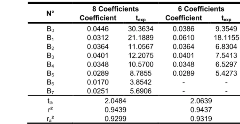
To obtain additional information, the results are exploited through the design of experiment. Following the F-test (analysis of variance), the models with 6 or 8 coefficients are significant. Tab. 39 gives the analysis of the coefficients. In the two cases, all the coefficients are significance because texp > tth. More ra² is better in the case where there are 6 coefficients. Thus, the chosen model is the one with 6 coefficients.
Tab. 39: Analysis of the significance of the effects in the cases of 8 or 6 coefficients
N° 8 Coefficients 6 Coefficients
Coefficient texp Coefficient texp
B0 0.0446 30.3634 0.0386 9.3549 B1 0.0312 21.1889 0.0610 18.1155 B2 0.0364 11.0567 0.0364 6.8304 B3 0.0401 12.2075 0.0401 7.5413 B4 0.0348 10.5700 0.0348 6.5297 B5 0.0289 8.7855 0.0289 5.4273 B6 0.0170 3.8542 - - B7 0.0251 5.6906 - - tth 2.0484 2.0639 r² 0.9439 0.9437 ra² 0.9299 0.9319
Fig. 44 shows the interactions between the aggregates
and the binders. The lines of the corn cob extract and the black liquor are confused. Their impact is the same on the thermal conductivity for these two aggregates. The slope of the lines for the composites, whatever the binder, is more important than the slope of the line in the case of the bulk. The interaction between the hemp shiv and the binders is the same except for the PLA where the interaction is more important. The interaction between the corn cob residues and the binders is not the same. Indeed, it is more important for the flax fines extract and less important for the lignin BioChoice®.
Fig. 44 : Interaction graph for the thermal conductivity (W.m-1.K-1)
For an identical production process, Fig. 45 shows that thermal conductivity increases when the hemp shiv are replaced by the corn cob residues (B1 coefficient) and when the bulk is converted into composites (B2, B3, B4 and B5 coefficients). Indeed, the density of the composites increases with the use of corn cob residues as aggregates. The binder with the least important impact is the lignin (B5 coefficient). The corn cob extract (B2 coefficient) and the black liquor (B4 coefficient) both have high impact on the thermal conductivity (nearly the same). The path diagram gives the flax fines extract the highest impact. However, the impact of flax fines extract is much higher on corn cob composites than on hemp shiv composites. Indeed, the impact induced by flax fines extract is not only due to the type of binder but also to its effect on composite density.
Fig. 45: Path diagram for the thermal conductivity (W.m
-1.K-1)
3.2 Hygric characterization
Fig. 46 shows the ambient relative humidity and
temperature in the climate chamber during the test. The mean value of relative humidity is slightly lower than 75 % during absorption (about 71.4 %) and slightly higher than
33% during desorption (about 35.5 %) because the door of the climate chamber is regularly open to weight specimens (peak on the curve). The SHT 75 sensor is calibrated at 23°C using silica gel and saturated salt solutions at 22.75, 32.90, 43.16, 58.20, 75.36, 81.20 and 97.42 %RH. The relative humidity is then calculated with:
𝑹𝑯𝒄𝒐𝒓.= 𝟎. 𝟎𝟎𝟒𝟑 𝑹𝑯𝑺𝑯𝑻𝟕𝟓𝟐+ 𝟎. 𝟔𝟎𝟗𝟔 𝑹𝑯𝑺𝑯𝑻𝟕𝟓+ 𝟑. 𝟑𝟒𝟓𝟖 (7)
It is obtained from the calibration of sensor, which is realized with saturated salt solutions at 22.75, 32.90, 43.16, 58.20, 75.36, 81.20 and 97.42 %RH for a temperature of 23°C. The value of point zero is obtained with silica gel at 23°C.
Fig. 46: Monitored relative humidity and temperature in the climate chamber during MBV test
Fig. 47 gives as example the moisture uptake and release
of sample n°1. For all composites, the change in mass shows less than 5 % of discrepancy for cycles 3 to 5. The moisture buffer value is thus calculated from cycles 3 to 5.
Fig. 47: Moisture uptake and release for sample n°-1-A Fig. 48 to Fig. 51 summarize the moisture buffer values
obtained in absorption, desorption and on average. The standard deviations are low, leading to coefficients of variation lower than 4.5 %.
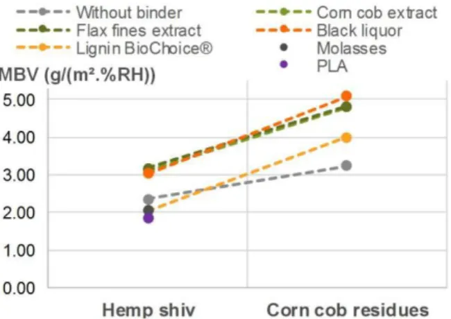
The average MBV range from 1.86 to 5.08 g/(m².%RH). According the Nordtest classification [Rode 2005], only the composite n°6 is good hygric regulators (1 < MBV < 2 g/(m².%RH)). The others composites are all excellent hygric regulators (MBV > 2 g/(m².%RH)).
As shown on Fig. 49 and Fig. 51, the moisture buffer value is not impacted by the density of composite. For a same binder, the composites made with corn cob residues have a better MBV than the composites made with hemp shiv. This is good sense because in bulk, the corn cob residues have already a better MBV than the hemp shiv.
The composites made from similar binders (corn cob extract, flax fines extract and black liquor) and hemp shiv,
have close MBV around 3.14 g/(m².%RH). It is the same with the composite made from similar binders (corn cob extract, flax fines extract and black liquor) and corn cob residues, they have close MBV around 4.90 g/(m².%RH). The composite n°6, which has the lowest MBV (1.86 g/(m².%RH)), is made with hemp shiv and PLA. The others composites made from hemp shiv have a MBV slightly higher around 2.05 g/(m².%RH).
Thus, the MBV is impacted by the type of aggregate and of binder, not only by bulk density.
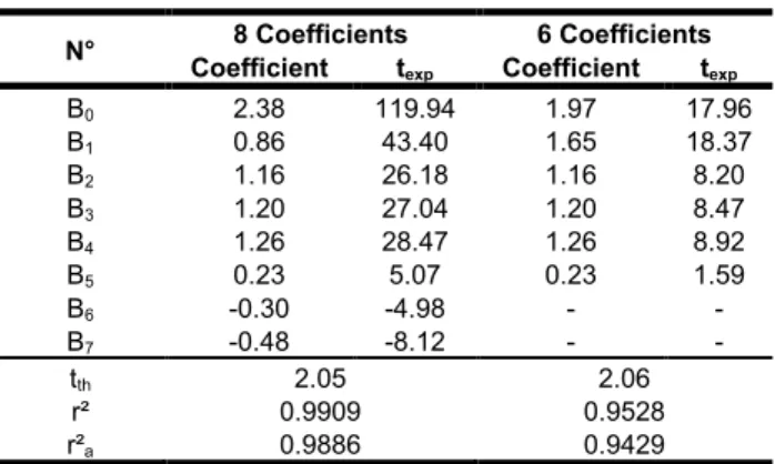
Tab. 40: Analysis of the significance of the effects in the cases of 8 or 6 coefficients
N° 8 Coefficients 6 Coefficients Coefficient texp Coefficient texp
B0 2.38 119.94 1.97 17.96 B1 0.86 43.40 1.65 18.37 B2 1.16 26.18 1.16 8.20 B3 1.20 27.04 1.20 8.47 B4 1.26 28.47 1.26 8.92 B5 0.23 5.07 0.23 1.59 B6 -0.30 -4.98 - - B7 -0.48 -8.12 - - tth 2.05 2.06 r² 0.9909 0.9528 r²a 0.9886 0.9429
To obtain additional information, the results are exploited through the design of experiment. Following the F-test (analysis of variance), the models with 6 or 8 coefficients are significant. Tab. 40 gives the analysis of the
coefficients. In the case there are 6 coefficients, the B5 coefficient is not significant because texp < tth. More ra² is better in the case there are 8 coefficients. Indeed, the adjustment quality of the model as measured by the adjusted determination coefficient is very good because it is close to 1. Thus, the chosen model is the one with 8 coefficients.
Fig. 52 shows the interactions between the aggregates
and the binders. The lines of the two extracts are confused. Their impact is the same on the MBV for these two aggregates. The slope of the lines for the black liquor and the lignin BioChoice® are the same. However, the interaction between the black liquor and the aggregates is better than the one of the lignin BioChoice®. The interaction between the hemp shiv and the extracts binders and the black liquor, is the same. The interaction between the hemp shiv and the others binders is less important as the synergy is negative. The interaction between the corn cob residues and the binders is not the same. Indeed, it is more important for the black liquor and less important for the lignin BioChoice®.
Fig. 53 shows that MBV increases when the hemp shiv
are replaced by the corn cob residues (B1 coefficient) and when the bulk is converted into composites (B2, B3, B4 and B5 coefficients). For the B6 and B7 coefficients, when the bulk is converted into composites, the MBV decreases. These binders should seal the pores of agro-resources. The binder which have the most important impact on the increasing of the MBV is the black liquor (B4 coefficient). The binder with the least important positive impact is the lignin BioChoice® (B5 coefficient). The corn cob extract (B2 coefficient) and the flax fines extract (B3 coefficient) have
Fig. 48: Moisture buffer value versus composites based on hemp shiv
Fig. 49: Average moisture buffer value of composites based on hemp shiv (g/(m².%RH)) versus density
Fig. 50: Moisture buffer value versus composites based on corn cob residues
Fig. 51: Average moisture buffer value of composites based on corn cob residues (g/(m².%RH)) versus density
nearly the same impact on the MBV. This impact is somewhat less important than the one of black liquor.
Fig. 52: Interaction graph for the moisture buffer value (g/(m².%RH))
Fig. 53: Path diagram for the moisture buffer value (g/(m².%RH))
4 CONCLUSION
This study shows that it is possible to produce wholly bio-based composites. Indeed, use these combinations of binders and aggregates is very interesting from the environmental perspective because local agriculture is given priority, waste and by-products are used in the production of these binders and none additive is added. The density of developed composites ranges from 177 to 273 kg/m3 with hemp shiv as aggregates, and ranges from 457 to 557 kg/m3 with corn cob residues as aggregates. The thermal conductivity ranges from 0.0675 to 1.479 W.m-1.K-1. It is mainly dependant on density but it is also slightly impacted by the type of binder. Thus, the composites made with hemp shiv have a lower thermal conductivity than the ones made with the corn cob residues.
The composites are all excellent hygric regulators (MBV > 2 g/(m².%RH)) except the composite made with PLA,
which is only a good hydric regulator. For a same binder, the composites made with corn cob residues have a better MBV than the composites made with hemp shiv. More, the use of the molasses and the PLA decreases the MBV because these binders should seal the pores of agro-resources.
Further research is still required to qualify the durability and the fire resistance of such composites and to study other properties such as the mechanical performances. Actually, mechanical properties are highly interesting on several points of view: handling, cutting and performance in use.
5 ACKNOWLEDGEMENTS
This project has received funding from the European Union’s Horizon 2020 research and innovation program under grant agreement No. 636835 – The authors would like to thank them.
CAVAC, industrial partner of the ISOBIO project, is gratefully acknowledged by the authors for providing raw materials.
Thanks are due to Tony Hautecoeur.
6 REFERENCE
[Collet 2016] Collet, F.; Pretot, S.; Lanos, C.; Hemp-straw composites: thermal and hygric performances, ICOME, 2016, Place: La Rochelle, France.
[Glassco 1987] Glassco, R.B.; Noble, R.L.; Modular building construction and method of building assembly, WO1987003031 A1, 1986.
[Goupy 2006] Goupy, J.; Creighton, L.; Introduction aux plans d’expériences, Dunod, 2006, ISBN978-2-10-049744-7.
[Oehlert 2000] Oehlert, G.W.; A first course in design and analysis of experiments, New York, W.H. Freeman, 2000, ISBN978-0-7167-3510-6.
[Rabier 2007] Rabier, F.; Modélisation par la méthode des plans d’expériences du comportement dynamique d’un module IGBT utilisé en traction ferroviaire, Location: Toulouse, Institut National Polytechnique, PhD Thesis, 2007.
[Rode 2005] Rode, C.; Peuhkuri, R.H.; Mortensen, L.H.; Hansen, K.K. and al; Moisture buffering of building materials, Technical University of Denmark, Department of Civil Engineering, 2005.
[Sun 2000] Sun, R.C.; Tomkinson, J.; Essential guides for isolation/purification of polysaccharides, Academic Press: Lond, 2000.
[Viel 2017] Viel, M.; Collet, F.; Lanos, C.; Chemical and hygrothermal characterization of agro-resources’s by-product as a possible raw building material, ICBBM, 2017, Place: Clermont-Ferrand, France.