HAL Id: hal-02637331
https://hal.inrae.fr/hal-02637331
Submitted on 27 May 2020
HAL is a multi-disciplinary open access
archive for the deposit and dissemination of
sci-entific research documents, whether they are
pub-lished or not. The documents may come from
teaching and research institutions in France or
abroad, or from public or private research centers.
L’archive ouverte pluridisciplinaire HAL, est
destinée au dépôt et à la diffusion de documents
scientifiques de niveau recherche, publiés ou non,
émanant des établissements d’enseignement et de
recherche français ou étrangers, des laboratoires
publics ou privés.
Distributed under a Creative Commons Attribution| 4.0 International License
formosat-2 satellite image time series
David Sheeren, Mathieu Fauvel, Veliborka Josipovic, Maïlys Lopes, Carole
Planque, Jerome Willm, Jean-François Dejoux
To cite this version:
David Sheeren, Mathieu Fauvel, Veliborka Josipovic, Maïlys Lopes, Carole Planque, et al.. Tree species
classification in temperate forests using formosat-2 satellite image time series. Remote Sensing, MDPI,
2016, 8 (9), 29 p. �10.3390/rs8090734�. �hal-02637331�
Tree Species Classification in Temperate Forests Using
Formosat-2 Satellite Image Time Series
David Sheeren1,*, Mathieu Fauvel1, Veliborka Josipovi´c1, Maïlys Lopes1, Carole Planque1, Jérôme Willm1and Jean-François Dejoux2
1 DYNAFOR, INP-ENSAT, INP-EI Purpan, INRA, University of Toulouse, Auzeville 31320, France;
[email protected] (M.F.); [email protected] (V.J.); [email protected] (M.L.); [email protected] (C.P.); [email protected] (J.W.)
2 CESBIO, CNES, CNRS, IRD, UPS, University of Toulouse, Toulouse 31401 Cedex 9, France;
* Correspondence: [email protected]; Tel.: +33-5-34-32-39-81 Academic Editors: Randolph H. Wynne and Prasad S. Thenkabail
Received: 30 June 2016; Accepted: 30 August 2016; Published: 7 September 2016
Abstract: Mapping forest composition is a major concern for forest management, biodiversity assessment and for understanding the potential impacts of climate change on tree species distribution. In this study, the suitability of a dense high spatial resolution multispectral Formosat-2 satellite image time-series (SITS) to discriminate tree species in temperate forests is investigated. Based on a 17-date SITS acquired across one year, thirteen major tree species (8 broadleaves and 5 conifers) are classified in a study area of southwest France. The performance of parametric (GMM) and nonparametric (k-NN, RF, SVM) methods are compared at three class hierarchy levels for different versions of the SITS: (i) a smoothed noise-free version based on the Whittaker smoother; (ii) a non-smoothed cloudy version including all the dates; (iii) a non-smoothed noise-free version including only 14 dates. Noise refers to pixels contaminated by clouds and cloud shadows. The results of the 108 distinct classifications show a very high suitability of the SITS to identify the forest tree species based on phenological differences (average κ=0.93 estimated by cross-validation based on 1235 field-collected plots). SVM is found to be the best classifier with very close results from the other classifiers. No clear benefit of removing noise by smoothing can be observed. Classification accuracy is even improved using the non-smoothed cloudy version of the SITS compared to the 14 cloud-free image time series. However conclusions of the results need to be considered with caution because of possible overfitting. Disagreements also appear between the maps produced by the classifiers for complex mixed forests, suggesting a higher classification uncertainty in these contexts. Our findings suggest that time-series data can be a good alternative to hyperspectral data for mapping forest types. It also demonstrates the potential contribution of the recently launched Sentinel-2 satellite for studying forest ecosystems. Keywords:tree species; forest; time series; classification; smoothing; Whittaker; phenology; biodiversity
1. Introduction
Forest ecosystems provide essential services to human society. Beyond the production of multiple resources (timber, energy, foods), these ecosystems play a major role in carbon sequestration, regulating biogeochemical cycles and climate [1]. However, the provision of such ecosystem services may depends on tree species diversity [2]. The complementarity among species can sustain multiple services simultaneously. Mapping tree species is therefore crucial to assess forest ecosystems and their services. Under the current context of climate change, it is also essential to build more accurate models predicting future tree habitat shifts [3]. Information about tree species diversity is required to assess forest resilience and vulnerability to drought and pathogens [4,5].
While important advances in the knowledge of global tree cover and its change have been reported recently [6], little is known about the current composition of forests at large scale [7]. Existing maps of tree species are often derived from species distribution models (SDM) which provide potential geographic ranges of tree species but not the exact geo-location of the species [8,9]. These models give projections of the ecological niches of species using a set of habitat indicators (such as climatic, edaphic and topographic variables) and a set of species observations, often based on National Forest Inventory plot data [10,11].
An alternative to the SDM-based approach for mapping tree species is the use of earth observation imagery. Tree species identification is a classical topic in optical remote sensing of forests [12,13]. Many studies have already addressed this issue in different ways. However, obtaining an accurate tree species classification is still a challenging task. A large number of factors influences the spectral response of species such as leaf biochemical properties, canopy structure, forest density and maturity, illumination and acquisition conditions. Thus, the spectral variability within species may be sometimes higher than the variability between species.
In the past, much attention has been devoted to the spatial resolution of the data [14]. Aerial photography have been the most frequently used data for forest inventory including the estimation of forest composition [15,16]. Discrimination of tree species was often based on visual interpretation, relying on the fine spatial details provided by this data and on the stereoscopic vision. Automated methods have been developed [17,18] including textural analysis [19,20] or canopy height models from stereo-images [21] to improve classification accuracy. In general, results show a limited success with potentially high confusion rates (>20%–30%).
The emergence of the very high spatial resolution (VHR) sensors has increased the number of works on tree species classification. New studies focused on the spatial details to map individual trees in temperate or tropical forest environments [22–24]. These studies are in line with the first attempts based on the high-resolution multispectral sensors like Landsat TM [25,26]. Despite some encouraging results, the reduced number of spectral bands in these images cannot allow an accurate species discrimination when only one image is available.
Alternatively, several authors investigated the ability to identify tree species using airborne hyperspectral imagery [27–30], LiDAR data [31] or a combination of multiple sources [32–35]. Spectral variability between species related to differences in biochemical properties are better preserved using hyperspectral data which allow continuous sampling of the electromagnetic spectrum. Incorporating LiDAR-derived information on height and canopy structure to hyperspectral responses of vegetation can also improve the classification of tree species [33,36]. The simultaneous use of these sources have demonstrated a high potential for species discrimination with accuracies higher than 90%. However, the operational use of these data remains difficult because of their limited availability and high cost.
A third approach for the classification of individual tree species is the use of optical multitemporal imagery. In this approach, phenological variations from green-up to senescence are assumed to increase the spectral separability between species. The use of multi-seasonal images has been successfully applied in several previous works. However, most of them were based on Landsat data composed of a limited number of dates, sometimes acquired from different years, and covering partially the key phenological periods [25,37–40]. Relatively few studies have attempted to assess the potential of dense high spatial resolution satellite image time series (SITS) for mapping forest types. SITS with very high frequency of observations such as MODIS have been already tested but the coarse spatial resolution of the images makes the tree species identification difficult in the case of complex forest environment [41]. The previous experiments were based on NDVI temporal profiles which help to reduce the data dimensionality but can also limit the discrimination between species. Using high resolution airborne images, [42,43] showed promising results at finer spatial resolution but they also highlighted the influence of the number of spectral bands and the number of dates on classification performance, in addition to the timing of image acquisition during the stages of leaf flush, leaf tinting
and fall. More recently, [44] investigated the ability of intra-annual image time series of RapidEye (6.5 m pixel size) to identify the most frequent tree genera in the urban environment of Berlin, Germany. The authors observed a decrease in quantity disagreement and allocation disagreement for data with higher temporal and spectral resolution.
In this paper, we explore the benefits of using a very dense high spatial resolution multispectral Formosat-2 image time-series for mapping 13 tree species in temperate forests. Compared to previous studies, the available time-series data composed of 17 dates acquired across one year, with constant viewing angles, is unique. The specific aims of the paper are:
• Develop an optimal classification strategy for mapping tree species in natural forests and tree plantations at three class hierarchy levels using dense Formosat-2 SITS.
• Quantify the effect of removing noise (i.e., clouds and cloud shadows) in the time series on classification accuracy.
• Identify the best supervised learning classifier among parametric and nonparametric methods. • Evaluate the sensitivity of the classification accuracy to the dimensionality of the data and to
the feature space, by comparing the classification results based on different feature sets: spectral bands, NDVI index or spectral bands and NDVI.
This study should demonstrate the potential contribution of the recently launched Sentinel-2 satellites for studying forest ecosystems. Formosat-2 and Sentinel-2 have close sensor characteristics in the visible and near-infrared spectral domain (similar spatial and spectral resolutions with close period of revisit).
2. Study Area and Data 2.1. Study Site
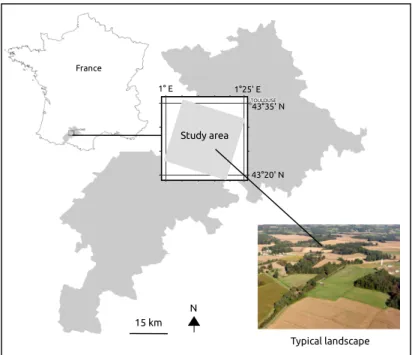
The study site is located in southwest France (Figure 1), in the Garonne river floodplain, approximately 30 km west of Toulouse (1◦100E, 43◦270N). It is a rural landscape within a sub-Atlantic climate characterized by mild and rainy winters with warm and dry summers (average annual temperature>13◦C ; annual precipitation = 656 mm). Woodlands cover less than 10% and are dominated by Oak. Non-forest areas consist of a combination of crops (including wheat, sunflower and maize) and grasslands.
15 km Typical landscape France 1°25' E 1° E 43°20' N 43°35' N Study area N
2.2. Image Data and Forest Map
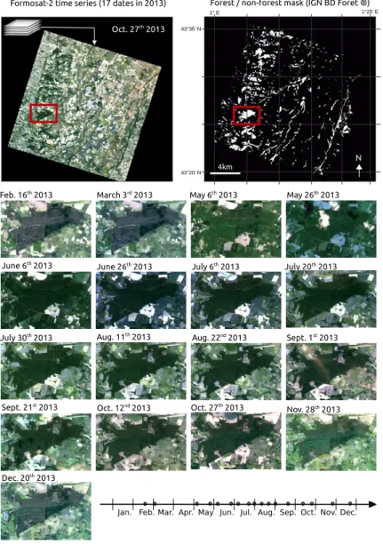
Formosat-2 optical imagery was used for this study. The time series has been acquired in the framework of the VENµS mission preparation that results from a cooperation between the Israeli Space Agency (ISA) and the French Centre National d’Etudes Spatiales (CNES) [45]. The Formosat-2 SITS was acquired on 17 dates in 2013 (Figure2). The multispectral images provide 4 spectral bands from the visible (Blue: 0.45–0.52 µm, Green: 0.53–0.60 µm, Red: 0.63–0.69 µm) through the near-infrared (NIR: 0.76–0.90 µm) at 8-m spatial resolution with a field of view of 24 km. The radiometric resolution of the data is 8-bit. All the images were acquired with the same constant viewing angle which is likely to reduce the within-species spectral variation.
An ancillary vector map was also used to mask the non-forest areas. These data were derived from the French National Forest Inventory database (IGN BD Foret®, v.1) produced in 1996. This database provides a forest/non-forest map with a minimum forest area (i.e., the minimum mapping unit) of 2.25 hectares (Figure2). Because of a temporal mismatch between the SITS (year 2013) and the ancillary map (year 1996), the forest data layer was manually updated, based on the SITS and aerial photographs.
Feb. 16th 2013 March 3rd 2013 May 6th 2013 May 26th 2013
June 6th 2013 July 6th 2013 July 20th 2013 July 30th 2013 Aug. 11th 2013 June 26th 2013 Oct. 12nd 2013 Aug. 22nd 2013 Sept. 1st 2013 Sept. 21st 2013 Nov. 28th 2013 Dec. 20th 2013
Jan. Feb. Mar. Apr. May Jun. Jul. Aug. Sep. Oct. Nov. Dec.
Forest / non-forest mask (IGN BD Foret ®) Formosat-2 time series (17 dates in 2013)
Oct. 27th 2013 Oct. 27th 2013 N 4km 1°25' E 1° E 43°35' N 43°20' N
Figure 2. Dataset used in the study composed of a multispectral Formosat-2 time series of 17 dates covering a 24 km×24 km area and a forest/non-forest mask derived from the French National Forest Inventory database. The Formosat images with excerpts focusing on one forest are viewed in true color composites.
2.3. Field Data
Four specific surveys were conducted across the study site in November 2013, January 2014, May 2014 and October 2015 to collect sample points (n=1235) of the most dominant broadleaf and conifer tree species. Each plot was recorded by two observers on pure stands covering approximately an extent of 576 m2(i.e., nine contiguous Formosat pixels of 8 m×8 m). Plots were distributed over the whole study site (51 distinct forests) and their location were assessed using a Garmin GPSMap 62st receiver (±3–5 m accuracy). The field-collected data did not include the young generation of trees (age<15 years). Class errors in this reference dataset were estimated to be less than 2%. Because of possible mix of species at the plot borders (due to the GPS inaccuracy), we only used the pixel at the center of the nine contiguous pixels in the calibration and validation procedures of the supervised classification. Thus, all the plots were converted into homogeneous polygons of one pixel size.
Three thematic levels were defined (Table1). The first level split the forests into broadleaf and conifer species (level 1). The second one makes distinction between four groups of species including deciduous and evergreen broadleaves species, pines and the other conifer species (level 2). The last one includes twelve distinct species and one group of three species of the same genus (level 3). This hierarchy was inspired from the French National Forest Inventory database nomenclature adapted to visual interpretation of aerial photographs [46]. Sample size per species varied from 51 pixels for Willow to 209 pixels for Aspen.
Table 1. Class hierarchy composed of three levels with the sample size of collected reference data (in pixels ; n =1235) for all the tree species. Each sample represents the pixel at the center of nine contiguous pixels of the same species.
Level 1 Level 2 Level 3 Sample Size
Broadleaf Deciduous Silver birch (Betula pendula) 85
Broadleaf Deciduous Oak (Quercus robur/pubescens/petraea) 113
Broadleaf Deciduous Red oak (Quercus rubra) 145
Broadleaf Deciduous European ash (Fraxinus excelsior) 80
Broadleaf Deciduous Aspen (Populus tremula) 209
Broadleaf Deciduous Black locust (Robinia pseudoacacia) 59
Broadleaf Deciduous Willow (Salix spp.) 51
Broadleaf Evergreen Eucalyptus (Eucalyptus spp.) 148
Conifer Pine Corsican pine (Pinus nigra subsp. laricio) 62
Conifer Pine Maritime pine (Pinus pinaster) 87
Conifer Pine Black pine (Pinus nigra) 55
Conifer Other conifer Douglas fir (Pseudotsuga menziesii) 66
Conifer Other conifer Silver fir (Abies alba) 75
3. Methods
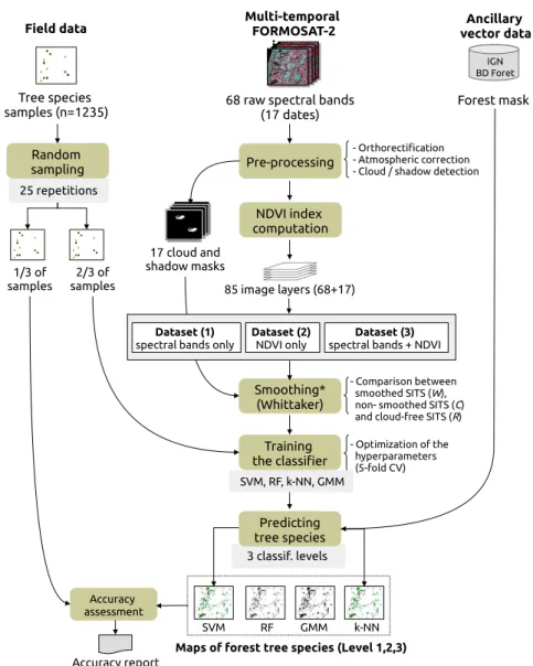
The processing chain defined to discriminate tree species using Formosat-2 SITS included several steps (Figure3). First, orthorectification, atmospheric correction and cloud detection was performed using an operational pre-processing chain, called MACCS (Multi-sensor Atmospheric Correction and Cloud Screening), resulting in (i) surface reflectance time-series data; and (ii) masks of clouds and cloud shadows [47,48]. In this chain, atmopheric effects are corrected by combining multi-temporal and multi-spectral criterion to estimate aerosol optical tickness [48] while clouds are detected by analyzing the reflectance increase in the blue spectral band [49]. Then, NDVI index was computed for each date (Figure3). Three image datasets were derived: one including the spectral bands only (68 image layers; dataset 1), another one including the NDVI index only (17 image layers; dataset 2) and the last one including both the spectral bands and NDVI (85 image layers; dataset 3). In the next step, each of these datasets was smoothed to deal with noisy pixels (i.e., cloudy and shady). The Whittaker smoothing algorithm (see Section3.1) was applied on the SITS in which, for each date, pixels affected by cloud coverage and cloud shadows were marked as missing values, using the cloud
and shadow masks. Then, a part of field data on tree species was used to train several supervised classifiers: Support Vector Machines (SVM), Random Forest (RF), Gaussian Mixture Model (GMM) and k-Nearest Neighbors (k-NN). The remaining field data samples on tree species were used to assess the classification performance of the models. In order to evaluate the effect of smoothing and noisy data on classification accuracy, the procedure was repeated on (i) the non-smoothed image datasets contaminated by clouds or cloud shadows (i.e., with the original reflectance values in the cloudy and shady areas); and (ii) on image datasets with no cloud or cloud shadow on forests (14 dates instead of 17 dates). Finally, all the results were compared to conclude on the best classification strategy. The key steps of the method are detailed below.
Field data Multi-temporal FORMOSAT-2 images
68 raw spectral bands (17 dates) Ancillary vector data Forest mask NDVI index computation 85 image layers (68+17) Pre-processing 2/3 of samples 1/3 of samples Tree species samples (n=1235) Predicting tree species
Maps of forest tree species (Level 1,2,3)
RF GMM Accuracy assessment Accuracy report - Orthorectification - Atmospheric correction - Cloud / shadow detection
- Optimization of the hyperparameters (5-fold CV) 25 repetitions IGN BD Foret 3 classif. levels Predicting tree species k-NN 17 cloud and shadow masks Smoothing* (Whittaker) Training the classifier SVM Random sampling Dataset (2) NDVI only Dataset (1)
spectral bands only spectral bands + NDVIDataset (3)
- Comparison between smoothed SITS (W), non- smoothed SITS (C) and cloud-free SITS (R)
SVM, RF, k-NN, GMM
Figure 3. Tree species classification process of the Formosat-2 satellite image time series. Note that the smoothing step is applied on the three datasets separately (*).
3.1. Smoothing of Temporal Profiles
Optical dense time series are often affected by noise due to clouds and shadows. In this study, noisy pixels were marked as missing values and the resulting temporal profiles were corrected using the Whittaker smoother [50]. This smoother has been selected for its fast execution, its limited number of parameters (only one) and its ability to deal with missing values [51].
Let z(ti), the value of one observed (noisy) pixel at time i for a given spectral band of the
SITS of length T = {t1, t1, ..., tn}. The vector composed of each observed value of the pixel in
the SITS is denoted by z = {z(t1), ..., z(tn)}. The noise free (unobserved) version is denoted by
x= {x(t1), ..., x(tn)}. The related noise model is such as: z = x+nwhere n follows a zero mean
normal distribution.
The Whittaker smoother algorithm is based on penalized least squares with the basic principle that smoothing must be a compromise between fidelity to the data (denoted by S in Equation (1)), and roughness of the smoothed curve (denoted by Rd). More precisely, the objective of the smoother is to
find ˆx such as it minimizes, with respect to x, a function Q(x)which combines the two conflicting goals: ˆx=arg min
x
Q(x)where Q(x) =S(x) +λRd(x) (1)
The fidelity S is expressed as the sum of the squared differences between observed pixels z(ti)
and smoothed pixels x(ti):
S(x) =
n
∑
i=1
(z(ti) −x(ti))2 (2)
The measure of roughness Rdis the norm of derivatives. It can be expressed, in its discrete
form, as the squared sum of the differences∆dx(ti), where∆dx(ti)represents a d order difference of
a pixel x(ti): Rd(x) = n
∑
i=1 (∆dx(ti))2 (3)Regularization parameter λ in Equation (1) is a smoothing parameter defined by the user. The larger it is, the smoother ˆx will be (increasing the lack of fit to the data). Here, the value of λhas been estimated by ordinary (OCV) and generalized (GCV) leave-one-out cross validation. OCV and GCV were computed for a series of values of λ={100, ..., 1015} to search for a minimum of it.
Since we had missing values in the data at each date because of clouds and shadows, a vector of weights w (with the same size of z) was introduced in S with w(ti) =0 for missing values and
w(ti) =1 for non-missing values. This information was derived from the 17 cloud and shadow masks.
Expressed in matrix notation, it took the form: S(x) =
n
∑
i=1
w(ti)(z(ti) −x(ti))2= (z−x)>W(z−x) (4)
where W is a n×n matrix with vector w on its diagonal.
A version of Whittaker smoother adapted for unequally spaced data was used since the time period between two consecutive images in the SITS was not constant. In this version, S was estimated in the same way as for an equally spaced data with missing values. The measure of the roughness of x was given by:
Rd(x) = n
∑
i=1 (∆dx(t i))2= Ddx 2 =x>Dd>Ddx (5)where Dd is the derivative matrix of order d. Finding partial derivatives of the final function Q in
Equation (1) and setting them to zeros leads to the following solution:
ˆx= (W+λDd>Dd)−1Wz (6)
3.2. Training and Validating the Models
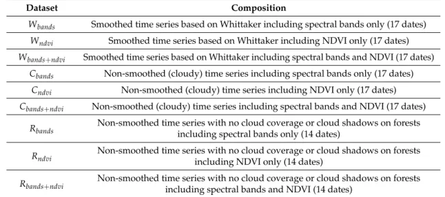
Classifications were carried out on nine datasets (Table2) corresponding to the cross product between the stacked images of spectral bands alone, ndvi alone, and both spectral bands and ndvi with (i) the smoothed version of the SITS (17 dates, dataset W); (ii) the non-smoothed version of the SITS
with cloudy images (17 dates, dataset C); and (iii) the non-smoothed version of the SITS including only the cloud-free and cloud shadow-free images on forests (14 dates, dataset R, a subset of C).
Table 2. Datasets used to evaluate the influence of the spectral features and the smoothing on the classification accuracy.
Dataset Composition
Wbands Smoothed time series based on Whittaker including spectral bands only (17 dates)
Wndvi Smoothed time series based on Whittaker including NDVI only (17 dates)
Wbands+ndvi Smoothed time series based on Whittaker including spectral bands and NDVI (17 dates)
Cbands Non-smoothed (cloudy) time series including spectral bands only (17 dates)
Cndvi Non-smoothed (cloudy) time series including NDVI only (17 dates)
Cbands+ndvi Non-smoothed (cloudy) time series including spectral bands and NDVI (17 dates)
Rbands Non-smoothed time series with no cloud coverage or cloud shadows on forestsincluding spectral bands only (14 dates)
Rndvi Non-smoothed time series with no cloud coverage or cloud shadows on forests
including NDVI only (14 dates)
Rbands+ndvi Non-smoothed time series with no cloud coverage or cloud shadows on forestsincluding spectral bands and NDVI (14 dates)
All the classifiers were computed using the scikit-learn Python library [52]. SVM was used with a gaussian Radial Basis Function (RBF) kernel given its superior performance compared to other kernels [53]. Adequate values of the hyperparameters were selected after testing ranges of values using a grid search. Ranges were specified as follows: the regularization parameter C={1, 10, ..., 105} and the width of the RBF kernel function γ={2−5, ..., 25}. For RF, we varied the number of classification trees from 10 to 500 (step = 50). For k-NN, the spectral similarity between the unlabeled pixels and the reference pixels was measured as Euclidean distance in the feature space. The optimal value of k, the number of nearest neighbors, was selected in the range from 1 to 50 (step = 5). For GMM, a regularization was introduced in the inversion of the covariance matrix with a parameter varying from 10−8to 108(step = 1 for the power value). All the hyperparameters of each method have been selected using a 5-fold cross validation.
The classifiers were trained using 2/3 randomly selected reference pixels per class (i.e., using an equal sample rate for each class by stratified sampling), and the learning models were validated using the remaining independent pixels (1/3). Classifications were carried out after masking the non-forest areas using ancillary data. Confusion matrices with overall accuracy and kappa statistics were computed and averaged over 25 repetitions (i.e., by applying the repeated random data-splitting procedure). Finally, comparisons of performance between classifiers and datasets were carried out statistically, based on the Wilcoxon rank-sum nonparametric test, and spatially, based on map comparison.
4. Results
Statistical results of the classifications are reported in Figure4. For each classifier, the kappa index is plotted for the three levels of the class hierarchy and the accuracy is provided for all the image datasets (27 tests per classifier).
In general, the results revealed a very high potential of Formosat-2 image time series to be used to discriminate forest tree species based on phenological differences. On average, a kappa (κ) value of 0.93 was obtained, all the classifiers, thematic levels and band combinations included (108 classifications). In most of the cases, an increase in thematic accuracy (from level 1 to level 3) has lead to a decrease in classification accuracy, with an average kappa value varying from 0.94 for level 1 to 0.91 for level 3.
However, the results exhibited a sensitivity to the spectral features, the smoothing and the classification algorithms. This sensitivity is analyzed in the following sections. For all the comparisons, difference in accuracy is declared significant when the p-value of the Wilcoxon rank test is less or equal to α = 0.05.
1 2 3 0.8 0.85 0.9 0.95 1 Class Level Kappa (a)GMM classifier 1 2 3 0.8 0.85 0.9 0.95 1 Class Level Kappa (b)SVM classifier 1 2 3 0.8 0.85 0.9 0.95 1 Class Level Kappa (c)RF classifier 1 2 3 0.8 0.85 0.9 0.95 1 Class Level Kappa (d)k-NN classifier
W bands W ndvi W bands ndvi C bands C ndvi C bands ndvi R bands R ndvi R bands ndvi
Figure 4. Average Kappa coefficient± standard deviation obtained after 25 repetitions for each classifier (GMM in (a), SVM in (b), RF in (c), k-NN in (d)) at the three levels of the class hierarchy (2 classes at level 1; 4 classes at level 2; 13 classes at level 3). The smoothed and non-smoothed versions of the SITS (17 dates) are denoted respectively by W (in blue) and C (in red). The non-smoothed cloud-free version of the SITS (14 dates) is denoted by R (in orange). Accuracy is provided for each group of spectral features: spectral bands alone (solid line), NDVI alone (dashed line), or spectral bands and NDVI (dotted line).
4.1. Influence of the Classifier
On average, considering all the nine datasets, SVM was found to be the best classifier at the three levels of the class hierarchy (Table3). GMM performed the worst at level 1 (κmean= 0.91). RF was the
less efficient at level 3 (κmean= 0.90). However, the results are close between the classifiers with only
partial significant differences (16/27 between SVM and k-NN, 24/27 between SVM and RF and 20/27 between SVM and GMM; Figure4). The highest κ values obtained with SVM were 0.98 using Rbandsat
level 1 (broadleaf vs conifer tree species), 0.97 using Wbandsat level 2 (4 classes of tree species), and 0.97
using Cbandsat level 3 (13 classes of tree species) (Figure4).
In most of the cases, as the classification becomes more specific from level 1 to level 3, the performance decreases significantly, especially using NDVI alone (Figure4). This is true for SVM, RF and k-NN, excepting GMM. At level 1, the GMM average accuracy based on the Wndvi, Cndviand Rndvidatasets
(κmean = 0.83 ± 0.02; Figure4) is lower than the ones at level 2 (κmean = 0.88 ± 0.02) and level 3
species at level 1 is more difficult than learning a greater number of more homogeneous classes at levels 2 and 3, in particular, when only a subset of spectral features available is used.
Table 3.Accuracy comparison between the classifiers based on the average kappa values±standard deviation computed from the results of all the nine datasets.
GMM SVM RF k-NN
Level 1/all datasets 0.91±0.02 0.96±0.01 0.93±0.02 0.95±0.01 Level 2/all datasets 0.93±0.01 0.95±0.01 0.93±0.01 0.94±0.01 Level 3/all datasets 0.92±0.01 0.93±0.01 0.90±0.01 0.91±0.01 4.2. Influence of the Spectral Features
Except for RF, there is no significant benefit of adding NDVI to spectral bands to discriminate tree species. The kappa values are very close whatever the classifier (GMM, SVM, k-NN) and the level of the class hierarchy (Figure4). In the case of RF, incorporating NDVI has only a slight but significant positive effect on classification accuracy for levels 1 and 2 (∆kmean = 1%). By contrast, the classification
performance decrease significantly using NDVI alone for all the classifiers (e.g.,∆kmean= 6% between
bands-based and ndvi-based classifications of level 1 with SVM). 4.3. Influence of the Smoothing
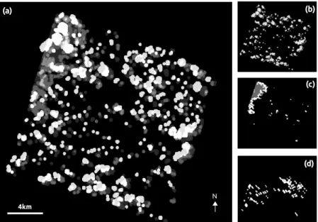
Smoothing was performed to remove cloud contamination in the data. A large proportion of the pixels of the SITS were impacted by clouds and cloud shadows (Figure5). The most affected images are those one acquired in 26 May (14.3% of the entire image), 20 July (4.9%) and 21 September (3.9%). Considering only the reference plots, 397 pixels were affected by cloud contamination at least once (i.e., 32% of the sample size). Twelve of the thirteen species were concerned. However, if we only focus the analysis on forests, fourteen images of the SITS were non-cloudy and non-shady. Clouds and cloud shadows on forests appear in 26 May, 1 and 21 September.
4km 4km (a) (b) (c) (d) N
Figure 5. Resulting graylevel image of clouds and cloud shadows combining all the individual masks of the SITS at each date (a); or detected only in 26 May (b); in 20 July (c); and in 21 September (d). The grayscale intensity vary from black (cloud and shadow free) to white (maximum of clouds and shadows).
The smoothing effect can be evaluated by comparing the performance of the three groups of datasets W, C and R (Figure4). In the experiments, the optimal value for the regularization parameter λ of the Whittaker smoother was estimated to 105from both Generalized and Ordinary Cross-validation. This parameter value has been retained to smooth all the W datasets.
In a general way, there is no difference in accuracy between the classifications based on the smoothed and non-smoothed datasets at level 1, except for RF. With this classifier, the non-smoothed datasets C or R perform slightly but significantly better than W (∆kmean = 1%). This is also true for SVM
and k-NN using NDVI alone (∆k≥2% between Wndviand Cndvi) . At level 2, a decrease in classification
accuracy is observed with the R dataset. The non-smoothed C dataset performs significantly better for most of the classifiers, especially using NDVI alone. No significant differences appear between the C and W datasets using the spectral bands alone or the spectral bands combined with NDVI, except for RF. At level 3, differences in accuracy between the datasets increase. The R dataset including only the 14 cloud-free and shadow-free images is the worst. Thus, the results are improved when all the dates are added in the SITS, even if the time series contains noisy data, as the C dataset. In some cases, the C dataset performs significantly better than the smoothed W dataset. This is true for all the classifiers using NDVI alone. This also appears for RF and k-NN using spectral bands alone or spectral bands with NDVI.
4.4. Confusions between Species
A confusion matrix summarizes the results for the best classification at level 3 based on the SVM classifier and the smoothed Wbandsdataset (Table4) (see AppendixAfor values in pixels). Among
the broadleaf tree species, Silver birch, Red oak, Eucalyptus, European Ash, Aspen and Willow showed the highest accuracies (confusion rate<1%). Oak and Black locust were the most difficult to discriminate (confusion rates equal to 5.03% and 3.05% respectively). Oak is mainly confused with Silver birch (1.64%) and Eucalyptus (1.44%). For Black locust, confusions were observed with Oak (2.29%). Considering conifer species, the best agreement was obtained for Silver fir (96.77%). Douglas fir showed the lowest accuracy (87.13%). The main confusions appeared with Silver fir (6.78%). The other important classification errors were observed between the three Pine species and Pines with Oak. In a general way, more confusions were observed among conifer tree species compared to broadleaf tree species which is consistent with the fact that phenology is less informative for conifers than deciduous tree species (see AppendixB).
The final results of forest type mapping are shown in Figure6. According to our field observations, the dominant species in the small forests is Oak. Conifer species are located in the biggest forests including some deciduous species. Red oak, Eucalyptus and Aspen (tree plantations) are mainly present in isolated homogeneous patches.
4.5. Classification Stability
In spite of the optimal accuracy estimated from the confusion matrix, an in-depth analysis of the cartographic results revealed a high instability between the classifiers, especially at level 3. When the class value predicted by each classifier was compared, for each pixel, classification consistency was found at level 1 for most of the pixels (96.5% of agreement between 3 or 4 classifiers). Similar results were computed at level 2 (94.5% of agreement). However, a high ambiguity was observed at level 3 with only 11.1% of pixels in agreement between all the classifiers and 55.6% of agreement between 3 classifiers (mainly SVM, RF and k-NN). The highest instability was observed in the core of complex forests including various deciduous or conifer species. Disagreements between the classifiers were also found in forest edges. By contrast, a high consistency appeared within monospecific broadleaf plantations at the three levels of the class hierarchy, in particular, for Red Oak, Aspen and Eucalyptus.
Table 4. Confusion matrix between the 13 tree species (level 3) computed in % and averaged over 25 repetitions. The matrix is based on the best classification obtained using the smoothed Wbands dataset and the SVM classifier. Rows and columns represent pixels in the classification and the reference respectively. The class labels are: 1 (Silver birch), 2 (Oak), 3 (Red oak), 4 (Douglas fir), 5 (Eucalyptus), 6 (European Ash), 7 (Aspen), 8 (Corsican pine), 9 (Maritime pine), 10 (Black pine), 11 (Black locust), 12 (Silver fir), 13 (Willow).
Reference Class Predicted Class 1 2 3 4 5 6 7 8 9 10 11 12 13 1 100 1.64 0.08 0 0 0 0 0 0 0 0 0 0 2 0 94.97 0.08 0.52 0 0.43 0.22 1.45 2.27 3.80 2.29 0 0 3 0 0.51 99.84 0 0 0 0 0 0 0 0 0 0 4 0 0 0 87.13 0 0 0 1.45 0 0 0 1.54 0 5 0 1.44 0 0.52 99.76 0 0 0 0 0 0 0 0 6 0 0.62 0 0 0 99.00 0.06 0 0 0 0.76 0 0 7 0 0.10 0 0 0 0.57 99.72 0 0 0 0 0 0 8 0 0.62 0 0.35 0 0 0 93.64 3.07 2.11 0 0 0 9 0 0.10 0 2.43 0.24 0 0 2.91 91.73 0.63 0 0 0 10 0 0 0 2.26 0 0 0 0.55 1.87 93.46 0 1.69 0 11 0 0 0 0 0 0 0 0 0 0 96.95 0 0 12 0 0 0 6.78 0 0 0 0 0 0 0 96.77 0 13 0 0 0 0 0 0 0 0 1.07 0 0 0 100 2 km Level 3 Silver birch Oak Red oak Doulgas fir Eucalyptus European ash Aspen Corsican pine Maritime pine Black pine Black locust Silver fir Willow 1° E 1°20' E 43°30' N 43°25' N N
Figure 6. Map of forest tree species at level 3 based on the smoothed Wbandsdataset and the SVM classifier. Excerpts of image in false color infrared are derived from the winter Formosat-2 image acquired in 16 Februrary 2013. At this time, a clear distinction between conifer and deciduous tree species is observed.
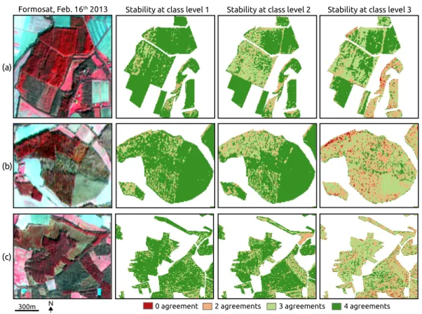
Examples of classification stability are given in Figure7. The first one shows tree plantations composed of Aspen (Figure7a, in the southwest) and Eucalyptus (Figure7a, in the center and the north). A good agreement is observed between the classifiers at the three thematic levels. The other two examples show mixed forests composed of conifers (Douglas fir and Corsican pine in Figure7b; Maritime pine and Douglas fir in Figure7c) with deciduous species (Oak in both examples with Silver birch in Figure7b). In these two cases, instability between the classifications is high at level 3, especially for mixed pixels and heterogeneous forest edges. These patterns were found for all the datasets used.
This comparison between the classifiers suggested overfitting of the models at level 3. Indeed, when the same similarity analysis was performed using only the reference pixels (n = 1235), 97.6% of agreement between 3 or 4 classifiers was found. In order words, the models had a high explanatory power at level 3 but a weak predictive performance. Except for broadleaf tree plantations, an overestimation of the classification accuracy is assumed for complex forests, regarding the dissimilarities between the maps of forest types.
Stability at class level 3 Stability at class level 2
Stability at class level 1 Formosat, Feb. 16th 2013
0 agreement 2 agreements 3 agreements 4 agreements
300m
(a)
(b)
(c)
N
Figure 7. Degree of relative agreement between the SVM, RF, k-NN and GMM classifiers at the three classification levels using Wbandsdataset. Stability is observed at level 3 for monospecific tree plantations in (a) compared to complex forests with mixed pixels in (b) and (c).
5. Discussion
Globally, the results showed a high suitability of Formosat-2 multispectral SITS for mapping detailed forest types in temperate woodlands. High classification accuracies were obtained from several classifiers highlighting the importance of phenological information for discriminating various broadleaf and coniferous tree species. To the best of our knowledge, this is the first study examining the potential contribution of dense (17 dates) high spatial resolution (<10 m) image time series to classify several tree species in temperate forests within a complete seasonal cycle of vegetation.
Regarding the classifiers, SVM outperforms RF, k-NN and GMM. This finding is consistent with previous studies focusing on forest applications [33,54]. SVM often produces higher classification
accuracy than the traditional methods, especially when small training samples are available and when the data are of high dimensionality [55,56]. However, to obtain the best accuracy, SVM supposes to select the adequate kernel with the optimal values of the hyperparameters. The number of user-defined parameters is higher than the other classifiers. In terms of computational time, the method is also slower, especially for predictions. For GMM based on NDVI datasets, when the number of classes increases from level 1 to level 2, an increase in accuracy is observed, contrary to the other classifiers. This is due in large part to the Gaussian assumption of the Maximum Likelihood estimation. At level 1, since the normal distributions of the two classes are defined from the pixels of all the conifer and broadleaf species, they are characterized by a high variability in reflectance that may not handle multimodal distributions well. In this case, GMM requires to define more classes (i.e., the subclasses) to better estimate the data distributions [57]. The non-parametric methods such as SVM or RF are more flexible since they do not require any assumptions about data distribution.
Regarding the spectral features, adding NDVI to the spectral bands has not significant effect on the classification performance. This is probably due to the fact that NDVI is a function of the red and near-infrared spectral bands and thus, is highly correlated to these bands. Conversely, using NDVI alone decreases significantly the classification accuracy, even though a lower number of features is used (i.e., the data dimensionality is reduced). This suggests that the differences in the seasonal dynamic of NDVI are too slight among some tree species. Larger differences are found using all the spectral bands (see AppendicesBandC).
Regarding the smoothing, we did not found any clear benefit of removing noise in the data using the Whittaker smoother. When NDVI is used alone, the non-smoothed dataset outperforms the smoothed one. These findings contradict other previous studies that evaluated the effect of noise reduction in time series data before classification. Some authors found improved inter-class separability after smoothing using Whittaker algorithm [51,58]. Nevertheless, smoothing has not always a positive effect. As revealed by [58] for crop-specific classification, smoothing may also reduce classification accuracy. If the smoothing process is excessive, removing all the roughness of the raw data, the inter-class separability may be affected. In our study, the smoothing parameter λ has been adjusted automatically by cross-validation (CV) in a fixed range of values (from 100 to 1015). As suggested by a visual inspection of the temporal profiles before and after smoothing
(see AppendixD), the optimal value we computed by CV may be adapted in some cases (i.e., producing a stronger smoothing).
Another important point highlighted by our results is the fact that the classification performance is improved using all the 17 dates in the SITS instead of including only the 14 cloud-free images, even if the full SITS contains noisy data (i.e., non-smoothed images with cloud contaminated pixels). One explanation for this is the small number of dates affected by clouds and cloud shadows in the SITS. More than 32% of the reference plots was found to be related to noisy pixels but for most of them, in only one image (26 May). Thus, the negative effect of noisy data is lower than the benefit of adding more dates in the SITS. The inclusion of the three cloudy images on forests (26 May, 1 September, 21 September) improves the separability between the classes. This is especially true for conifer tree species, as revealed by the comparison of the confusion matrix. The additional dates enable the confusions to be reduced between Douglas fir and Corsican pine (−5%) as well as between the three classes of pines. For deciduous species, no notable changes were observed in classification accuracy, suggesting that no additional phenological information was provided with the supplementary images. Despite the very high performance we found statistically, the classification stability analysis between the classifiers has shown uncertainties at level 3, in particular, for non-plantations in mixed forests. An overestimation of accuracy is assumed for these cases. This assumption is supported by the important difference in accuracy between our analysis and the previous studies focusing on tree species mapping using multitemporal images. A difference of 17% of kappa is observed with the best results obtained by [43] to classify six deciduous tree species (Ash, Aspen, Birch, Elm, Maple, Oak) using a combination of five Airborne Thematic Mapper images. Our results also outperform the ones
reported by [42] to identify four species (Yellow poplar, White oak, Red oak and Red maple). These species were mapped at 76% overall accuracy (κ = 0.41) using a combination of four spectral bands and five of the nine dates available from aerial photographs. In another study, [38] discriminated 33 forest classes (20 dominant types with 13 sub-classes) with an overall accuracy of 79% based on multiseasonal Landsat TM data. More recently, an intra-annual time series of RapidEye data including five dates was used to classify 8 tree genus in an urban environment [44]. Several classification scenarios were tested to evaluate the impact of phenological information and the RapidEye’s red edge band on the accuracy. The best classification they achieved using SVM was estimated to 83% of kappa.
Although these previous studies are not directly comparable because they were conducted with different methods and imagery, for different tree species, the strong classification performance we obtained for 13 species (average kappa of 93% at level 3 with SVM) is surprisingly much higher, suggesting a potential bias in the learning procedure and the accuracy assessment. This bias could be explained by several reasons: (1) overfitting; (2) classification of data with imbalanced class distribution; (3) the use of only pure pixels for training and validating the classifications; (4) a discrimination restricted to the most dominant tree species; (5) a partial spatial dependence between training and validation data.
Overfitting is suspected in our experiments regarding the high number of features relative to the small number of learning samples. For some classes, the number of features is greater than the sample size. In this case, overfitting is likely to occur, providing a model with a high explanatory power but a poor predictive performance (as suggested by the spatial comparison of the four classifier results). The sample size is known to be one of the most important factors affecting the quality of a model and its ability to generate accurate predictions. In the remote sensing community, several recommandations have been proposed to estimate the appropriate sample size although no clear consensus exists [59,60]. The required sample size depends on several factors including the classification algorithm but also the complexity of the learning problem. As a rule of thumb, [59] suggests to collect a minimum of 50 samples for each category. In this study, eight categories contain less than 85 pixels for training and validation. Because of the high dimensionality of our image datasets (when all the spectral bands are included), our sample sizes were probably too small to avoid overfitting and evaluate the classification accuracy properly, especially at level 3. As recommended with small reference datasets, cross-validation was retained to estimate the accuracy. Regularization was also introduced, but these efforts were probably insufficient. In order to prevent overfitting, one option may be to augment the ground-based reference dataset and to analyze the impact of larger training subsets on classification error (plotting the learning curve of the classifiers [57]). However, gathering additional reference data is costly and highly time-consuming. Adapted classification approaches enabling training set size to be reduced [61], or enabling training samples to be added iteratively, including unlabeled pixels [40], could be another option. Beyond these strategies to control sample size, overfitting could be also moderated using fewer features. The dimensionality of the data could be reduced from feature extraction or selection techniques [62,63]. The use of NDVI instead of the spectral bands is also an alternative, as we did. In this case, a decrease in classification accuracy should be observed with the decrease of overfitting. This may be another explanation of the lower performance we obtained for the classifications produced using NDVI alone.
The variation in the sample size across classes may also influence the rate of classification errors [64]. Samples of smaller classes can be misclassified more often than those belonging to prevalent classes. This could lead to an accuracy paradox: a less accurate model (in terms of overall accuracy) may be more useful than a more accurate one. Indeed, an excellent accuracy may be obtained by always predicting the prevalent classes with any prediction of the minority classes. In our study, the class imbalance is weak (maximum class size ratio of 4:1). In addition, we selected the kappa coefficient as a performance metric since kappa is more appropriate than the overall accuracy with imbalanced class distributions. Nevertheless, the minority classes were often the most confused (e.g., Black locust and Black pine). A part of the confusions appeared with the prevalent classes (e.g., Oak). This variation
in the sample size across classes is rather common for tree species classification [65], reflecting the uneven distribution of species abundances on landscape. Several solutions exist to overcome this problem, both at data level and algorithm level [64]. These include many different forms of resampling (oversampling the small classes, undersampling the prevalent classes, generating new synthetic data). Cost-sensitive learning approaches may be also adopted, assuming higher misclassification costs with samples in the minority class.
As revealed by classification instability at forest edges (often composed of a high variability of species), another cause of uncertainty may be the discrimination restricted to the most dominant tree species. In the studied forests, the number of species is higher than the 13 detected species. However, all the pixels were assigned to one of the dominant species. Thus, according to the classifier, pixels composed of non-sampled tree species may be assigned to different tree species classes. The non-sampled species (such as Hornbeam or Hazel tree) were too few to collect field data on them. Most of them were mixed with other species and spatially interspersed. Instability is also due to the presence of understory vegetation and the existence of harvesting operations in the forests during the year. Understory vegetation is visible in some images, after the leaf fall of the dominant trees. Clear cuts also appear in some forests (as observed in the excerpts of Figure2, from 30 July). This may also lead to differences in classification between the classifiers. The comparison of the classifiers should not be viewed as an accuracy assessment but rather as a similarity assessment that may be affected by various factors.
Since we processed a high spatial resolution SITS, we adopted a hard classification approach, assuming that all the pixels were pure in the forests. The results showed that this assumption was consistent in monospecific tree plantations. However, in the case of complex forest environments (Figure8), the proportion of mixed pixels was too high, generating dissimilarities between the classifiers at level 3. This result was not necessarily expected, the pixel size (8 m) being small enough to detect individual tree and thus, the variety of species within a single stand. Alternative approaches based on soft classification [66], spectral unmixing [67] or the use of small training sets containing mixed pixels [61] could be used to account for uncertainty in these forests.
(a) (b)
Figure 8. Examples of homogeneous and heterogeneous forest areas of the study site. At level 3, mixed forests show a high classification instability between the classifiers. (a) Monospecific forest composed of Silver birch; (b) Mixed forest composed of various deciduous and conifer species.
Finally, our evaluation method is independent, in the sense that pixels used to train and validate the classifications are strictly distinct. However, our random sampling design to select training and validation data (based on repeated split-sample) is not spatially constrained. Samples may come from the same geographic area or the same forests. Some species exist only in one forest. Other species appear in several forests but in various proportions. Thus, reference samples of tree species are not distributed equally over the forests. Consequently, the selection of reference samples for training and validation did not consider the effect of spatial autocorrelation among neighboring
pixels. Because close samples tend to have similar spectral values, this may influence the outcome of the supervised classification [68–71].
Despite these potential optimistic bias in accuracy assessment, the qualitative validation of our classifications, based on a visual interpretation of the maps and our field observations, confirmed the high level of classification accuracy computed for the most tree species. This high accuracy can be explained by the combination of the high spatial and temporal resolution of the Formosat-2 SITS, as well as the image acquisition at constant viewing angles which may reduce the within-species spectral variation. Phenological differences among the broadleaf tree species is also another factor explaining the performance obtained in this study (see the temporal profiles of each species in AppendicesBandC). The possible discrimination between Eucalyptus and the other broadleaf species is obvious, mainly due to the evergreen phenology of Eucalyptus. Red Oak is also unique, characterized by red leaves in spring (leaf out in May) and in autumn (leaf fall in November). The European ash phenology differs from the other broadleaf tree species by a shorter period with leaves (last tree to leaf out in May after flowering, first tree to drop leaves in late September). Between the other broadleaf species of the study, the leaf development starts with Aspen (early-mid of April), followed by Oak, Silver birch, Black locust and Willow (mid-late April until May). In autumn, the species senescence start with Aspen (late October), Black locust and Silver birch (early-mid of November), followed by Willow (yellow leaves) and Oak (late November, brown leaves).
6. Conclusions
Our study demonstrates the high suitability of dense optical high spatial resolution SITS for mapping dominant tree species in temperate woodlands. High classification accuracies (kappa>0.9) were obtained from several classifiers verifying the assumption that multispectral imagery makes tree species recognition possible when phenological information is taken into consideration. Specifically, we conclude from our findings that:
• The classification performance is slighlty influenced by the classifier. RBF-SVM classifier demonstrated the best accuracy at the three levels of the class hierarchy. GMM performed the worst.
• There is any clear benefit of removing cloudy and shady pixels using the Whittaker smoother in our context, even if 32% of the reference pixels were contaminated at least once. By contrast, adding all the dates in the SITS instead of only the cloud-free and shadow-free images enables the classification accuracy to be increased.
• There is no benefit of adding NDVI to spectral bands to discriminate tree species. By contrast, using NDVI alone led to a significant decrease in classification performance, even if the dimensionality of the data is reduced.
• Classification uncertainty exists for complex mixed forests, regarding the spatial disagreements that appear between the maps produced by all the classifiers. By contrast, a high consistency is observed within monospecific broadleaf plantations.
• Among the broadleaf tree species, Oak and Black locust are the most difficult to discriminate. For conifers, the lowest accuracy is observed for Douglas fir.
The conclusions of the study have to be taken with caution. Because of small sample size for some species, overfitting is suspected. Classification errors might also be affected by the imbalanced class distributions. Additional works should be carried out to confirm that the approach is transferable to other sites. Despite a possible overestimation of the predictive performance, we believe that these results provide the basis to map forest tree species across a broad spatial extent, using the forthcoming Sentinel-2 image time series. Further developments will be needed to better control the sampling and learning procedures. The spatial and temporal variability of tree species phenology at a regional or national scale should also be considered.
Our study is a first step towards the production of detailed and accurate maps of species composition for forest managers. These maps would also permit a variety of ecological applications.
Supplementary Materials:Full classification map is available online at http://goo.gl/bbzwZC.
Acknowledgments:This work was partially supported by the French Space Agency CNES (TOSCA OSO project). A special thanks to M. Huc and O. Hagolle from CESBIO for providing the pre-processed Formosat-2 time series with masks of clouds and cloud shadows.
Author Contributions:D.S. and M.F. conceived and designed the experiments; D.S., C.P., J.W. and J.-P.D. carried out the field work; V.J. and M.F. performed the experiments; M.L. implemented the smoothing method; D.S. and M.F. analyzed the data; D.S. wrote the paper with feedback from M.F., M.L. and J.-P.D.
Conflicts of Interest:The authors declare no conflict of interest.
Appendix A. Confusion Matrix in Pixels from the Smoothed WbandsDataset and the
SVM Classifier
Table A1. Confusion matrix between the 13 tree species (level 3) computed in pixels and averaged over 25 repetitions (explaining why there are decimal fractions). The matrix is based on the best classification obtained using the smoothed Wbandsdataset and the SVM classifier. Rows and columns represent pixels in the classification and the reference respectively. The class labels are: 1 (Silver birch), 2 (Oak), 3 (Red oak), 4 (Douglas fir), 5 (Eucalyptus), 6 (European Ash), 7 (Aspen), 8 (Corsican pine), 9 (Maritime pine), 10 (Black pine), 11 (Black locust), 12 (Silver fir), 13 (Willow).
Reference Class Predicted Class 1 2 3 4 5 6 7 8 9 10 11 12 13 1 29.00 0.64 0.04 0 0 0 0 0 0 0 0 0 0 2 0 37.04 0.04 0.12 0 0.12 0.16 0.32 0.68 0.72 0.48 0 0 3 0 0.20 49.92 0 0 0 0 0 0 0 0 0 0 4 0 0 0 20.04 0 0 0 0.32 0 0 0 0.40 0 5 0 0.56 0 0.12 49.88 0 0 0 0 0 0 0 0 6 0 0.24 0 0 0 27.72 0.04 0 0 0 0.16 0 0 7 0 0.04 0 0 0 0.16 71.80 0 0 0 0 0 0 8 0 0.24 0 0.08 0 0 0 20.60 0.92 0.40 0 0 0 9 0 0.04 0 0.56 0.12 0 0 0.64 27.52 0.12 0 0 0 10 0 0 0 0.52 0 0 0 0.12 0.56 17.72 0 0.44 0 11 0 0 0 0 0 0 0 0 0 0 20.36 0 0 12 0 0 0 1.56 0 0 0 0 0 0 0 25.16 0 13 0 0 0 0 0 0 0 0 0.32 0 0 0 16.00
Appendix B. Temporal Signatures in Each Spectral Band of the SITS for Each Broadleaf and Conifer Tree Species
Broadleaf Conifer 0 20 40 60 100 200 300 100 200 300
Day of the year (DOY)
R efl ectance (mean v alue in % * 10) Tree species Aspen Black locust Eucalyptus European ash Oak Red oak Silver birch Willow Corsican pine Maritime pine Black pine Douglas fir Silver fir Blue
(a) Blue band Figure B1. Cont.
Broadleaf Conifer 0 20 40 60 100 200 300 100 200 300
Day of the year (DOY)
R efl ectance (mean v alue in % * 10) Tree species Aspen Black locust Eucalyptus European ash Oak Red oak Silver birch Willow Corsican pine Maritime pine Black pine Douglas fir Silver fir Green (b) Green band Broadleaf Conifer 0 20 40 60 100 200 300 100 200 300
Day of the year (DOY)
R efl ectance (mean v alue in % * 10) Tree species Aspen Black locust Eucalyptus European ash Oak Red oak Silver birch Willow Corsican pine Maritime pine Black pine Douglas fir Silver fir Red (c) Red band Broadleaf Conifer 100 200 300 400 100 200 300 100 200 300
Day of the year (DOY)
R efl ectance (mean v alue in % * 10) Tree species Aspen Black locust Eucalyptus European ash Oak Red oak Silver birch Willow Corsican pine Maritime pine Black pine Douglas fir Silver fir Near Infrared
(d) Near infrared band
Figure B1.Average spectral signatures of the thirteen tree species in the blue (a), green (b), red (c) and near infrared (d) spectral bands of the SITS. Reflectance values (y-axis) are given for each day of the year (x-axis) in percent, multiplied by a factor of 10.
Appendix C. Boxplots of the NDVI Index of the SITS for Each Broadleaf and Conifer Tree Species 39 50 126 146 157 177 187 201 211 223 234 244 264 285 300 332 354 0.0 0.2 0.4 0.6 0.8 1.0 (a)Eucalyptus 39 50 126 146 157 177 187 201 211 223 234 244 264 285 300 332 354 0.0 0.2 0.4 0.6 0.8 1.0 (b)Silver birch 39 50 126 146 157 177 187 201 211 223 234 244 264 285 300 332 354 0.0 0.2 0.4 0.6 0.8 1.0 (c)Oak Figure C1. Cont.
39 50 126 146 157 177 187 201 211 223 234 244 264 285 300 332 354 0.0 0.2 0.4 0.6 0.8 1.0 (d)Red oak 39 50 126 146 157 177 187 201 211 223 234 244 264 285 300 332 354 0.0 0.2 0.4 0.6 0.8 1.0
(e)European ash
39 50 126 146 157 177 187 201 211 223 234 244 264 285 300 332 354 0.0 0.2 0.4 0.6 0.8 1.0 (f)Black locust Figure C1. Cont.
39 50 126 146 157 177 187 201 211 223 234 244 264 285 300 332 354 0.0 0.2 0.4 0.6 0.8 1.0 (g)Aspen 39 50 126 146 157 177 187 201 211 223 234 244 264 285 300 332 354 0.0 0.2 0.4 0.6 0.8 1.0 (h)Willow
Figure C1. Seasonal dynamic of NDVI distribution among broadleaf tree species: Eucalyptus (a), Silver birch (b), Oak (c), Red oak (d), European ash (e), Black locust (f), Aspen (g), Willow (h). Boxplots (medians and the interquartile range from 1st to 3rd quartiles) are defined for each date of the year (x-axis) of the Formosat-2 time series of 2013.
39 50 126 146 157 177 187 201 211 223 234 244 264 285 300 332 354 0.0 0.2 0.4 0.6 0.8 1.0
(a)Douglas fir
39 50 126 146 157 177 187 201 211 223 234 244 264 285 300 332 354 0.0 0.2 0.4 0.6 0.8 1.0 (b)Silver fir 39 50 126 146 157 177 187 201 211 223 234 244 264 285 300 332 354 0.0 0.2 0.4 0.6 0.8 1.0 (c)Corsican pine Figure C2. Cont.
39 50 126 146 157 177 187 201 211 223 234 244 264 285 300 332 354 0.0 0.2 0.4 0.6 0.8 1.0 (d)Maritime pine 39 50 126 146 157 177 187 201 211 223 234 244 264 285 300 332 354 0.0 0.2 0.4 0.6 0.8 1.0
(e)Black pine
Figure C2. Seasonal dynamic of NDVI distribution among conifer tree species: Douglas fir (a), Silver fir (b), Corsican pine (c), Maritime pine (d), Black pine (e). Boxplots (medians and the interquartile range from 1st to 3rd quartiles) are defined for each date of the year (x-axis) of the Formosat-2 time series of 2013.
Appendix D. Smoothing of Temporal Profiles Using Whittaker 50 100 150 200 250 300 350 0 50 100 150 200 250 300 350 400 D N V -V B l u e 50 100 150 200 250 300 350 0 50 100 150 200 250 300 350 D N V -V G r e e n 50 100 150 200 250 300 350 0 50 100 150 200 250 300 350 400 D N V -V R e d 50 100 150 200 250 300 350 0 100 200 300 400 500 600 700 800 D N V -V N e a r V I n f r a -R e d 50 100 150 200 250 300 350
DayV of V t heV year 0. 1 0. 2 0. 3 0. 4 0. 5 0. 6 0. 7 0. 8 0. 9 1. 0 D N V -V N D V I
(a)Pixel values affected by clouds in 26 May (DOY 146) and 20 July (DOY 201)
50 100 150 200 250 300 350 0 5 10 15 20 25 30 35 40 45 D N V -V B l u e 50 100 150 200 250 300 350 10 20 30 40 50 60 70 80 D N V -V G r e e n 50 100 150 200 250 300 350 0 10 20 30 40 50 60 70 80 90 D N V -V R e d 50 100 150 200 250 300 350 50 100 150 200 250 300 350 400 D N V -V N e a r V I n f r a -R e d 50 100 150 200 250 300 350
DayV of V t heV year 0. 50 0. 55 0. 60 0. 65 0. 70 0. 75 0. 80 0. 85 0. 90 D N V -V N D V I
(b)Pixel values affected by cloud shadows in 26 May (DOY 146) and 26 June (DOY 177)
Figure D1. Temporal profiles of spectral bands and NDVI for pixels affected by clouds (a) and cloud shadows (b) at several days of the year (DOY) in 2013. The noisy values of the pixels within the SITS are labeled in red. The cloud-free and shadow-free values of the pixels are represented in blue. The line represents the temporal profiles after application of the Whittaker smoother.
References
1. Assessment, M.E. Ecosystems & Human Well-Being: Synthesis; Island Press: Washington, DC, USA, 2005. 2. Gamfeldt, L.; Snall, T.; Bagchi, R.; Jonsson, M.; Gustafsson, L.; Kjellander, P.; Ruiz-Jaen, M.C.; Fröberg, M.;
Stendahl, J.; Philipson, C.D.; et al. Higher levels of multiple ecosystem services are found in forests with more tree species. Nat. Commun. 2013, 4, 1340.
3. Iverson, L.R.; McKenzie, D. Tree-species range shifts in a changing climate: Detecting, modeling, assisting. Landsc. Ecol. 2013, 28, 879–889.
4. Thompson, I.; Mackey, B.; McNulty, S.; Mosseler, A. Forest Resilience, Biodiversity, and Climate Change. A Synthesis of the Biodiversity/Resilience/Stability Relationship in Forest Ecosystems; Technical Series No. 43, Secretariat of the Convention on Biological Diversity: Montreal, QC, Canada, 2009.
5. Guyot, V.; Castagneyrol, B.; Vialatte, A.; Deconchat, M.; Selvi, F.; Bussotti, F.; Jactel, H. Tree diversity limits the impact of an invasive forest pest. PLoS ONE 2015, 10, e0136469.
6. Hansen, M.C.; Potapov, P.V.; Moore, R.; Hancher, M.; Turubanova, S.A.; Tyukavina, A.; Thau, D.;
Stehman, S.V.; Goetz, S.J.; Loveland, T.R.; et al. High-resolution global maps of 21st-century forest cover change. Science 2013, 342, 850–853.
7. Thompson, S.D.; Nelson, T.A.; White, J.C.; Wulder, M.A. Mapping dominant tree species over large forested areas using Landsat Best-Available-Pixel image composites. Can. J. Remote Sens. 2015, 41, 203–218.
8. Guisan, A.; Zimmermann, N.E. Predictive habitat distribution models in ecology. Ecol. Model. 2000,
135, 147–186.
9. Franklin, J. Mapping Species Distributions: Spatial Inference and Prediction; Cambridge University Press: Cambridge, UK, 2009.
10. Iverson, L.R.; Prasad, A.M.; Matthews, S.N.; Peters, M. Estimating potential habitat for 134 eastern US tree species under six climate scenarios. For. Ecol. Manag. 2008, 254, 390–406.
11. Brus, D.J.; Hengeveld, G.M.; Walvoort, D.J.; Goedhart, P.W.; Heidema, A.H.; Nabuurs, G.J.; Gunia, K. Statistical mapping of tree species over Europe. Eur. J. For. Res. 2012, 131, 145–157.
12. Holmgren, P.; Thuressopn, T. Satellite remote sensing for forestry planning — A review. Scand. J. For. Res.
1998, 13, 90–110.
13. Boyd, D.S.; Danson, F.M. Satellite remote sensing of forest resources: Three decades of research development. Prog. Phys. Geogr. 2005, 29, 1–26.
14. Nagendra, H. Using remote sensing to assess biodiversity. Int. J. Remote Sens. 2001, 22, 2377–2400. 15. Meyer, P.; Staenzb, K.; Ittena, K.I. Semi-automated procedures for tree species identification in high spatial
resolution data from digitized colour infrared-aerial photography. ISPRS J. Photogramm. Remote Sens. 1996, 51, 5–16.
16. Wulder, M.A.; Franklin, S.E. Remote Sensing of Forest Environments: Concepts and Case Studies; Kluwer Academic Publishers: Dordrecht, The Netherlands, 2003.
17. Brandtberg, T. Individual tree-based species classification in high spatial resolution aerial images of forests using fuzzy sets. Fuzzy Sets Syst. 2002, 132, 371–387.
18. Erikson, M. Species classification of individually segmented tree crowns in high-resolution aerial images using radiometric and morphologic image measures. Remote Sens. Environ. 2004, 91, 469–477.
19. Franklin, S.E.; Hall, R.J.; Moskal, L.M.; Maudie, A.J.; Lavigne, M. Incorporating texture into classification of forest species composition from airborne multispectral images. Int. J. Remote Sens. 2000, 21, 61–79. 20. Kayitakire, F.; Giot, P.; Defourny, P. Discrimination automatique de peuplements forestiers à partir
d’orthophotos numériques couleur: Un cas d’etude en Belgique. Can. J. Remote Sens. 2002, 28, 629–640. 21. Waser, L.T.; Ginzler, C.; Kuechler, M.; Baltsavias, E.; Hurni, L. Semi-automatic classification of tree species
in different forest ecosystems by spectral and geometric variables derived from Airborne Digital Sensor (ADS40) and RC30 data. Remote Sens. Environ. 2011, 115, 76–85.
22. Carleer, A.; Wolff, E. Exploitation of very high resolution satellite data for tree species identification. Photogramm. Eng. Remote Sens. 2004, 70, 135–140.
23. Immitzer, M.; Atzberger, C.; Koukal, T. Tree species classification with random forest using very high spatial resolution 8-band WorldView satellite data. Remote Sens. 2012, 4, 2661–2693.
24. Lin, C.; Popescu, S.C.; Thomson, G.; Tsogt, K.; Chang, C.I. Classification of tree species in overstorey canopy of subtropical forest using QuickBird images. PLoS ONE 2015, 10, e0125554.
25. Wolter, P.T.; Mladenoff, D.J.; Host, G.E.; Crow, T.R. Improved forest classification in the northern Lake States using multi-temporal Landsat imagery. Photogramm. Eng. Remote Sens. 1995, 61, 1129–1143.
26. Foody, G.M.; Hill, R.A. Classification of tropical forest classes from Landsat TM data. Int. J. Remote Sens.
1996, 17, 2353–2367.
27. Cochrane, M.A. Using vegetation reflectance variability for species level classification of hyperspectral data. Int. J. Remote Sens. 2000, 21, 2075–2087.
28. Féret, J.B.; Asner, G.P. Tree species discrimination in tropical forests using airborne imaging spectroscopy. IEEE Trans. Geosci. Remote Sens. 2012, 51, 73–84.
29. Ghiyamat, A.; Shafri, H.Z.; Mahdiraji, G.A.; Shariff, A.R.M.; Mansor, S. Hyperspectral discrimination of tree species with different classifications using single- and multiple-endmember. Int. J. Appl. Earth Obs. Geoinf.
2013, 23, 177–191.
30. George, R.; Padaliab, H.; Kushwahab, S.P. Forest tree species discrimination in western Himalaya using EO-1 Hyperion. Int. J. Appl. Earth Obs. Geoinf. 2014, 28, 140–149.
31. Heinzel, J.; Koch, B. Exploring full-waveform LiDAR parameters for tree species classification. Int. J. Appl. Earth Obs. Geoinf. 2011, 13, 152–160.