The CO
2
Content of Consumption
Across US Regions: A Multi-Regional
Input-Output (MRIO) Approach
Justin Caron, Gilbert Metcalf and John Reilly
Report No. 266
August 2014
The MIT Joint Program on the Science and Policy of Global Change combines cutting-edge scientific research with independent policy analysis to provide a solid foundation for the public and private decisions needed to mitigate and adapt to unavoidable global environmental changes. Being data-driven, the Program uses extensive Earth system and economic data and models to produce quantitative analysis and predictions of the risks of climate change and the challenges of limiting human influence on the environment—essential knowledge for the international dialogue toward a global response to climate change.
To this end, the Program brings together an interdisciplinary group from two established MIT research centers: the Center for Global Change Science (CGCS) and the Center for Energy and Environmental Policy Research (CEEPR). These two centers—along with collaborators from the Marine Biology Laboratory (MBL) at Woods Hole and short- and long-term visitors—provide the united vision needed to solve global challenges.
At the heart of much of the Program’s work lies MIT’s Integrated Global System Model. Through this integrated model, the Program seeks to: discover new interactions among natural and human climate system components; objectively assess uncertainty in economic and climate projections; critically and quantitatively analyze environmental management and policy proposals; understand complex connections among the many forces that will shape our future; and improve methods to model, monitor and verify greenhouse gas emissions and climatic impacts. This reprint is one of a series intended to communicate research results and improve public understanding of global environment and energy challenges, thereby contributing to informed debate about climate change and the economic and social implications of policy alternatives.
Ronald G. Prinn and John M. Reilly, Program Co-Directors
For more information, contact the Program office:
MIT Joint Program on the Science and Policy of Global Change Postal Address:
Massachusetts Institute of Technology 77 Massachusetts Avenue, E19-411 Cambridge, MA 02139 (USA) Location:
Building E19, Room 411 400 Main Street, Cambridge Access:
Tel: (617) 253-7492 Fax: (617) 253-9845
Email: globalchange@mit.edu
The CO2 Content of Consumption Across US Regions:
A Multi-Regional Input-Output (MRIO) Approach Justin Caron*†, Gilbert Metcalf *‡, John Reilly*
Abstract
We improve on existing estimates of the carbon dioxide (CO2) content of consumption across regions of
the United States. Using a multi-regional input-output (MRIO) framework, we estimate the direct and indirect CO2 emissions attributable to domestically and internationally imported goods. We include
estimates of bilateral trade between US states as well as between individual states and international countries and regions. This report presents two major findings. First, attributing emissions to states on a consumption versus a production basis leads to very different state-level emissions responsibilities; for example, when attributed on a consumption basis, California's per capita emissions are over 25 percent higher than when attributed on a production basis. Second, when attributing emissions on a consumption basis, heterogeneity of emissions across trading partners significantly affects emissions intensity. These findings have important implications for evaluating the potential distributional impacts of national climate policies, as well as for understanding differing incentives to implement state- or regional-level policies.
Content
1. INTRODUCTION ... 1
2. ESTIMATING THE CO2 CONTENT OF CONSUMPTION IN A MULTI-REGIONAL INPUT-OUTPUT MODEL ... 4
2.1 Defining Consumption-Based Emissions ... 4
2.2 Multi-Regional Input-Output ... 4
2.3 Consumption-Related Emissions ... 6
2.4 Emissions Intensity ... 7
3. RESULTS ... 9
3.1 Regional Emissions and Consumption-Based Emissions ... 12
3.2 Consumption: Household, Government and Investment Final Demand ... 14
3.3 The Direct and Indirect CO2 Intensity of Consumption ... 15
3.4 Understanding the Source of Differences in CO2 Intensity of Consumption ... 18
3.5 Importance of Accounting for International and Sub-National Trade Flows ... 21
4. CONCLUSIONS ... 22
5. REFERENCES ... 22
APPENDIX A – STATE-LEVEL RESULTS ... 24
APPENDIX B – DATA CONSTRUCTION ... 26
APPENDIX C – DECOMPOSITION ... 31
APPENDIX D – TRADE FLOWS ... 33
APPENDIX E – MRIO ILLUSTRATED WITH FLOW CHARTS ... 34
* Joint Program on the Science and Policy of Global Change, Massachusetts Institute of Technology, MA, USA. † Corresponding author (Email: jcaron@mit.edu)
1 1. INTRODUCTION
Extensive literature has been produced in attempts to trace the full effect of consumption patterns on carbon dioxide (CO2) emissions throughout the economy. There are many motivations for these studies, including attributing responsibility for emissions; guiding
producers, consumers, or public policy to favor products and processes with lower emissions; and understanding how emissions pricing might affect households with different consumption
patterns. One common approach relies on an engineering-based life-cycle approach that identifies emissions related to a particular production process, including emissions related to the production of inputs, and so forth, with the goal of identifying all emissions associated with a product
through its full life cycle (e.g. ISO, 2006; Liamsanguan and Gheewala, 2009; US EPA, 2010a, b; Jones and Kammen, 2011). Engineering-based analysis typically stops somewhere along the production chain; it will measure the direct emissions caused by producing chemicals which are used to produce a product of interest, but will not necessarily measure the emissions associated with building the plant producing the chemicals, or the emissions related to the cement used to build the plant producing the chemicals. A second common approach relies on input-output (I-O) tables, which describe the entire production chain. Linear algebra manipulation of I-O table matrices is commonly used to attribute emissions throughout the economy to individual consumption goods, and this manipulation does not arbitrarily truncate the emissions chain.1
While these two approaches are similar in some respects—and at some levels, have the same general goal—in application they generally have different purposes. Engineering life-cycle analysis is best suited to evaluate different brands of the same product, or different processes used to produce an otherwise homogeneous product. Life-cycle analysis can answer questions such as “Is cola A less CO2-intensive than cola B?” or “Is fuel production process X more CO2-intensive than fuel production process Y?” The I-O approach, on the other hand, is difficult to resolve at the level of different brands of the same product, or between different processes used to produce what otherwise is an otherwise homogeneous product, because of the relatively coarse level of aggregation in I-O tables. I-O analysis is better suited to indicate the full CO2 implications of the consumption patterns of different regions, or other large groups of consumers (e.g.,
households in different income classes). As such it can potentially be used to understand whether, for example, per capita emissions in California are low compared to those in Texas because Californians consume different products than Texans, or whether they are low because the emissions related to their consumption patterns are embodied in goods produced elsewhere and imported into the state. In that case, the full emissions effect of Californians’ consumption patterns may, in fact, be no different than that of Texans. One might attribute emissions from chemical and fuels production in Texas to Texans, and those emissions from the film industry in California to Californians, but it is possible that both Texans and Californians consume fuels and films at similar rates, resulting in similar indirect emissions.
1 This is a slightly different concept than “cradle to grave” accounting, which would also calculate emissions associated with the disposal of the product.
2
Apart from simply assigning responsibility, I-O analysis has also been used to assess the potential burden of emissions pricing on different consumers (e.g. Metcalf, 1999). Here, the idea is that a CO2 emissions price will be reflected in the cost of products throughout the economy in proportion to the emissions incurred during production. The price of final goods in the economy will thus reflect the CO₂ cost of their production and use, carrying along the cost of all the CO₂ emissions associated with intermediate and primary production. While I-O analysis is widely used for such purposes, such an assessment is at best an approximation, providing only a limited indication of which demographics may bear the burden of emissions pricing.
I-O analysis assumes that all industries have constant cost production functions, so all emissions costs are passed forward to consumers rather than backwards to owners of factors—which in general equilibrium is not the case. Wages and returns to assets will be affected—most likely differentially—by carbon pricing. Some households will derive more of their income from wages than capital, and among capital owners, some may be invested in fossil fuels while others are invested in renewable energy sources. I-O also assumes that there are no options to abate
emissions—which is the purpose of carbon pricing in the first place. A product whose production can be switched to a lower emitting process at minimal cost will do so, and therefore will not transfer much of the carbon price; a product with no reasonable low-carbon production options will have a much higher cost to pass forward (or backward). Even assuming all of these effects are neutral across households, these results do not address what happens with the revenue from, or allowance value inherent in, a carbon pricing system. How the revenue is used is often more important in determining the final distributional effects of a carbon pricing policy than the effects occurring through differential patterns of consumption (e.g., Rausch et al., 2010, 2011).
Nevertheless, current consumption patterns are one of the ingredients necessary to determine relative CO2 cost burden. Accurately measuring the CO2 consumption intensity is vital to our understanding of how burdens may differ across states and regions. Previously, in making such calculations for US states, studies have made the simplifying assumption that indirect emissions associated with the consumption of an imported product are uniform among different regional sources of the same product: a dollar’s worth of vehicle produced in Michigan has the same emissions as a dollar’s worth of vehicle produced in Tennessee, Germany, or Japan (e.g. Metcalf, 1999; Dinan and Rogers, 2002; Hassett et al., 2009; Mathur and Morris, 2012). This assumption was necessary because previous researchers lacked the full bilateral trade data needed to track domestic and international sources of imports. In recent studies, I-O modeling has been used to track CO2 emissions through the economy across countries, made possible by international trade data sets providing information on bilateral trade flows (see Wiedmann et al., 2007; Davis and Caldeira, 2010). It has also been used to compute the emissions embodied in trade across countries (e.g. Qi et al., 2014) and to compute the level of tariffs based on the total carbon intensity of imports (e.g. Winchester et al., 2011). Our contribution is to improve on empirical estimates for states or regions within the US—a timely issue, as recent Congressional efforts have focused on crafting legislation with mechanisms to “fairly” distribute the cost of a carbon policy among states.
3
We use the same terminology as Hassett et al. (2009), where direct emissions are defined as those related to household fuel use and the production of electricity used by households; all other emissions associated with consumption are termed indirect emissions. We define these terms more precisely in Section 2. Hassett et al. (2009) find that roughly half of CO2 emissions related to final consumption in the US are indirect emissions occurring in the production of non-energy goods consumed by households. While emissions associated with most non-energy goods and services are fairly low, the vast bulk of household spending goes toward purchase of these items2 and a large share of household emissions are thus embodied in non-energy goods and services.
One of our objectives for this study is to compare direct and indirect consumption-related emissions to production-based emissions, which are defined according to the point of emission, including all CO2 emitted within the region by both producers and consumers. Although we consider this to be the most natural metric for comparison with consumption emissions, we note that other metrics could be used to attribute emissions to states, such as accounting for “embodied production” emissions (attributing CO2 to states according to the point of extraction of fossil fuels). The relevance of each of these metrics depends on the locus of emission taxation: the direct
incidence of a downstream “consumption-based” tax would relate to consumption-based
accounting; production emissions would relate to a midstream tax based on the point of emissions; and a fully upstream tax would depend on the point of extraction of carbon.
To undertake this analysis, we develop a multi-regional input-output (MRIO) model with over 100 countries and the United States disaggregated to the state level. This allows us to track carbon embodied in imports and exports, as well as products domestically produced and consumed. We advance previous work by using available data for the US on interstate and international trade flows to estimate a full matrix of bilateral trade flows—both inter-state and between US states and foreign countries. While the full bilateral trade flow data are imperfect, we believe they allow us to challenge critical assumptions of previous work: specifically, that emissions intensities of similar goods imported from different regions are identical, and that measures of regional emissions are not appreciably distorted by the first assumption. If the difference in carbon intensity does not depend on the origin of imports into a state, then this simplifying assumption may be reasonable. However, if there are substantial differences among sources of imports, we can at least conclude that further data collection or effort to estimate bilateral trade flows is needed—either to develop better estimates, or to make a compelling case for assuming identical emissions intensities of imports.
In Section 2, we discuss the definition of “consumption” used in the analysis; we then describe the MRIO model and the data we used to compute CO2 content on a consumption basis. In Section 3 we discuss our findings. Two findings in particular stand out. First, attributing emissions to states on a consumption rather than production basis leads to very different state level emissions
responsibilities; for example, when attributed on a consumption basis, California's per capita emissions are over 25 percent higher than when attributed on a production basis. Second, when
2 Direct consumer expenditures on energy (fuel oil, natural gas, electricity and motor vehicle fuels) accounted for only 9% of household expenditures in 2011–2012. Data are from the Consumer Expenditure Survey Midyear Tables at http://www.bls.gov/cex/tables.htm, accessed on Aug. 5, 2013.
4
attributing emissions on a consumption basis, heterogeneity of emissions across trading partners significantly affects emissions intensity. We offer some final thoughts in Section 4.
2. ESTIMATING THE CO2 CONTENT OF CONSUMPTION
IN A MULTI-REGIONAL INPUT-OUTPUT MODEL 2.1 Defining Consumption-Based Emissions
In this study, we use a broad definition of consumption, including not only the final use of goods and services by private households, but also government and investment final demand. Goods and services purchased by state and federal governmental entities are assumed to benefit households within the same region, and we attribute the CO2 embodied in those goods to that region’s consumption. The attribution of emissions embodied in final investment demand introduces an additional level of complexity and is typically overlooked in the input-output literature. Ideally, we would relate emissions associated with past investment (in today’s capital stock) with current consumption; however, we cannot track the actual investments composing each sector’s current capital stock. While for this reason we cannot provide an accurate attribution of emissions over time, we can—with some assumptions—attribute current investment emissions to consumption in each region. We do so by sharing out each sector’s investment-related emissions proportionally to the destination regions of goods produced. More precisely, emissions associated with investment are a matter of timing attribution—a machine that is produced today is an input (with its associated emissions) in the future production of a stream of consumption goods. Accounting for emissions on a production basis is straightforward: emissions are counted at the location and time of production. When accounting on a consumption basis, however, we should prorate the emissions from the machine's production to the stream of consumption goods over time based on the machine's useful life. This could be approximated by measures of economic depreciation. In this study, we simply attribute the emissions to consumption at the time the machine is produced (equivalent in a depreciation sense to expensing the machine).
2.2 Multi-Regional Input-Output
We develop a multi-regional input-output (MRIO) model and use it to estimate the CO2
content of consumption across US regions. Input-Output models can track flows of inputs through the economy assuming Leontief production, and MRIO modeling has been widely used to track CO2 emissions through the economy and across countries. Wiedmann et al. (2007) provide a recent survey of that literature. To our knowledge, no previous studies on regional incidence of US carbon pricing policy have used MRIO modeling to determine differences in
CO2 consumption across regions of the US. Using the MRIO approach, we can track
emissions—on a consumption or production basis—through to final consumption, regardless of the origin of emissions or the number of intermediate production layers.3 For example, consider
3 Peters (2008) compares and contrasts production- and consumption-based emission methodologies based on an emissions embodied in bilateral trade (EEBT) approach and the MRIO approach. While the latter approach is more complex and less transparent, it is more accurate in allocating emissions to final consumption.
5
glass produced in Ohio that is exported to Michigan for assembly into automobiles, which in turn are exported to New York for sale. In consumption-based emissions accounting, the MRIO model allocates the emissions associated with the glass production to New York; under a production-based emissions framework, it would allocate the emissions to Ohio.
Our input-output framework also differs from what is found in existing literature on regional incidence of US carbon pricing policy in that it combines country-level data outside of the US with sub-national data within the US. In the context of this study, these two types of regions are conceptually similar, and we denote them with the same index r. The model tracks flows for n sectors of the economy. We follow the notation from previous literature, in particular Peters (2008). Output in region r (xr) is used in intermediate demand, final demand, and net exports:
𝑥!= 𝐴!𝑥!+ 𝑦!+ 𝑒!− 𝑚! (1)
where the n by n matrix Ar tracks the use of output 𝑥!as an intermediate input in region r, yr is a vector of dimension n of final demand in region r, er is a vector of exports from region r, and mr is a vector of imports to region r.
We create a decomposition according to the origin of intermediate and final demand. The input-output matrix Ar are decomposed into a matrix of industry requirements for domestic output (Arr) and matrices of industry requirements for production of domestic output from
imports from region s (Asr). Exports out of region r are decomposed according to their destination region s in the ers vectors, such that 𝑒! = 𝑒!"
!!! . Each of these are then decomposed into
exports for final demand in region s (yrs) and exports for use as intermediate inputs in region s (zrs):
𝑒!" = 𝑧!"+ 𝑦!" (2)
where
𝑧!" = 𝐴!"𝑥! (3)
Letting yrr represent the final demand in region r that is produced domestically, and noting that imports need not be tracked explicitly (since imports to region r from s are exports from region s to r), equation (1) can be rewritten as:
𝑥!= 𝐴!!𝑥!+ 𝑦!!+ 𝐴!"𝑥!
!!! + !!!𝑦!" (4)
This system of equations can be stacked over the R regions: 𝑥! ⋮ 𝑥! = 𝐴 !! ⋯ 𝐴!! ⋮ ⋱ ⋮ 𝐴!! ⋯ 𝐴!! 𝑥! ⋮ 𝑥! + 𝑦 !! ! ⋮ 𝑦!" ! (5) or X = AX + Y (6)
6
where X is an nR by 1 vector and so on. The Y vector is the vector of final demand both consumed domestically and imported.
The quantity of carbon dioxide emissions per unit of output associated with production in region r is denoted by the row vector fr of dimension n. These vectors can be stacked next to each other in the row vector F of dimension 1 by nR:
𝐹 = 𝑓!… 𝑓! (7)
2.3 Consumption-Related Emissions
Bilateral final demand in each region is represented by the nR vectors Yr: 𝑌!= 𝑦
!!
⋮ 𝑦!"
(8) As explained earlier, these final demand vectors are composed of final demand by private households Hr, government final demand Gr, and investment final demand Ir:
𝑌!= 𝐻!+ 𝐺!+ 𝐼! (9)
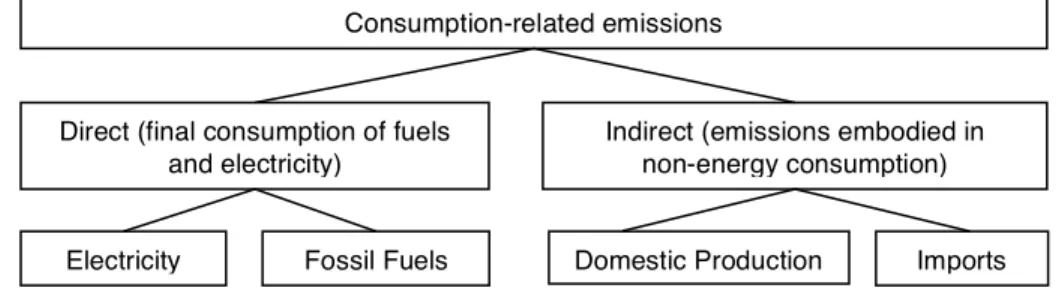
We now define the emissions associated with this final demand. Consistent with Hassett et al. (2009), we separate consumption-based emissions into direct and indirect emissions. Direct emissions are defined as emissions arising from household, government or investment fossil fuel demand, including emissions associated with the final demand for electricity. All other emissions embodied in final demand are categorized as indirect emissions (see Figure 1).
Specifically, direct household emissions are given by: 𝐸!,!"#! = 𝐵! 𝐻!+ 𝐸
!,!"!! (10)
where Br is a nR vector of CO2 emission coefficients representing the quantity of CO2 emitted per dollar of fossil fuel use by households in region r. The 𝐸!,!"!! term represents the emissions
associated with the electricity consumed by households.
Figure 1. Composition of consumption-related emissions.
Indirect emissions embodied in region r’s consumption are given by: 𝐸!,!"#$%! = 𝐹 𝐼 − 𝐴 !!𝐻!− 𝐸
!,!"!! (11)
Consumption-related emissions
Direct (final consumption of fuels and electricity)
Indirect (emissions embodied in non-energy consumption)
7
Total emissions associated with household consumption are the sum of direct and indirect emissions: 𝐸!! = 𝐸
!,!"#! + 𝐸!,!"#$%! . Direct and indirect emissions associated with government
and investment final demand (𝐸!! and 𝐸
!!) are computed in a similar manner. While we attribute
to each region the emissions associated with households and governments in that region, the emissions embodied in final investment demand (𝐸!!) are attributed to regions in proportion to the
final destination of the output of the sectors in which the investment occurred.
In our social accounting matrix, we observe final investment demand 𝐼! (the value of each
sector’s output going to investment) as well as capital earnings in each sector I, 𝑉!!. We assume
that investment per sector is proportional to capital earnings and use capital earnings to share out the CO2 embodied in investment (𝐸!!) to each sector. Assuming that investment in each sector has
the same CO2 intensity as aggregate investment, we compute 𝐸!!", the investment-related
emissions embodied in each sector: 𝐸!!" = !!!
!!!
! 𝐸!
! (12)
We then attribute investment emissions to regions according to the destination of each sector’s output. We assume that each region’s future production will be exported to the same distribution of destinations as current production. This share is computed using the elements of the inverted A matrix, 𝛼!,!,!,!, as 𝜃!,!,! = !,!!𝛼!,!,!,!!𝑦!,!!,!, assigning production in each sector to the region in which it will ultimately be consumed. These shares are used to compute the emissions embodied in investment for domestic production in region r as 𝐸!"! = 𝜃
!,!,!
! 𝐸!!", and the emissions
embodied in imported investment as 𝐸!!! = 𝜃
!,!,!𝐸!!"
!,! .
Finally, emissions embodied in region r’s consumption are the sum of household consumption emissions, government consumption emissions, and investment related emissions (both domestic and imported):
𝐸!! = 𝐸
!! + 𝐸!!+ 𝐸!"! + 𝐸!!! (13)
We will compare these emissions to regional production emissions (the CO2 emitted within region r), which include the emissions caused by the burning of fossil fuels in final demand as well as emissions in production:
𝐸!! = 𝐵! 𝑌!+ 𝑓!𝑥! (14)
2.4 Emissions Intensity
From the total emissions embodied in consumption (𝐸!!) we can compute the CO
2 intensity of consumption 𝑘!! as:
𝑘!! = !!!
!!"
8
The measure of CO2 intensity is closely related to the notion of carbon tax incidence computed in Hassett et al. (2009). Indeed, if the price shock caused by a tax on CO2 emissions is assumed to completely pass through to consumers, the two metrics are equivalent.
Here, we estimate the carbon content of consumption using MRIO, providing two
improvements on previous work. First, we account for differences in the CO2 intensity of foreign imports and trace these to a destination state or region of the US, taking into account whether they are consumed in that region or then traded to other parts of the country. Second,
intra-national trade patterns are based on interstate trade data, rather than assuming an homogeneous dispersion of products within the country.
Construction of the A, Y, and F matrices is discussed in Appendix B, and more detail is available in Caron and Rausch (2013). The resulting dataset used for the analysis includes input-output tables, final demand data and bilateral trade data for all 50 US states as well as 113 countries and regions outside of the US (see Table B3) for 2006. The dataset also includes the full matrix of bilateral trade between all regions of the US and their international trading partners, as well as CO2 emission coefficients for all regions. Our bilateral trade matrix does not, however, distinguish between trade in intermediate and final goods. Similar to other MRIO analyses, these are shared out according to bilateral trade shares. To our knowledge, there is no data describing shares of intermediate trade at the sector- and state-level.
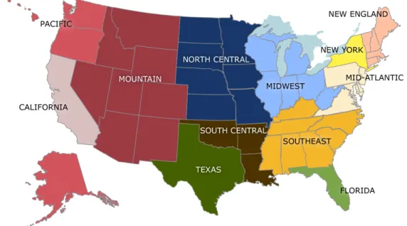
Because the dataset we have constructed covers the global economy, we are able to compute the total CO2 intensity of both internationally and domestically traded goods. Within states and countries, we track 52 sectors (see Table B2) including agricultural, industrial, service and energy goods. While we also compute results at the state level, we simplify exposition in the main body of this report by aggregating states to 12 regions, as shown in Figure 2.
Figure 2. Regional aggregation of US states. New England (NENG): ME, NH, VT, MA, CT, RI. Southeast (SEAS): KY,
NC, TN, SC, GA, AL, MS. Mid-Atlantic (MATL): DE, MD, PA, NJ, DC, VA. Midwest (MWES): WV, WI, IL, MI, IN, OH. South Central (SCEN): OK, AR, LA. North Central (NCEN): MO, ND, SD, NE, KS, MN, IA. Mountain (MOUN): MT, ID, WY, NV, UT, CO, AZ, NM. Pacific (PACI): OR, WA, HI, AK. Single-state regions: CA, FL, NY, TX.
9 3. RESULTS
Our main objective is to investigate differences in the CO2 intensity of consumption across regions of the US. We start by presenting the emission intensities of production across US regions and sectors, as these data provide the foundation for determining emissions embodied in consumption. Combining production emissions intensities with bilateral patterns of trade between the regions, we calculate inventories of consumption-based emissions between regions. We then compare these inventories to standard emission inventories based on emissions occurring within each region. Then, we allocate CO2 intensity of consumption according to the destination of final demand. Unless otherwise stated, all results are based on data from 2006.
We begin in Table 1 by reporting the average amount of CO2 (in kg) embedded in each dollar of gross output—the CO2 intensity of output—across regions of the US for the 24
highest-emitting sectors in the dataset (representing over 90 percent of US emissions). The intensity measure is the total amount of CO2 required for the production of goods in each sector, divided by the value of gross output in that sector. We could use this calculation to determine, for example, that for the Motor Vehicles/Parts sector in the Midwest region, $1 USD worth of output embodies an average of 0.58 kg of CO2. This number takes into account the use of intermediate inputs purchased both domestically and internationally.
Table 1 reveals heterogeneity in carbon intensities across both regions and sectors. For example, New England and New York have less than half the carbon content per dollar of Electricity output than the Southeast and Central regions. The distribution of intensities is more homogenous in other sectors but large differences exist in almost all goods and services. These reflect differences in technology, prices and the within-sector composition of production (these intensity measures use value as a denominator) as well as in the CO2 intensity of intermediate inputs, Electricity in particular.
These sector-level intensity measures can be used to investigate the distribution of impacts that may be caused by various carbon taxation policies. For example, if emissions were subject to a uniform tax t everywhere in the world (measured in terms of $USD per kg), one could use this intensity measure to compute a first-order approximation of the effect of such a tax on the price of any good by multiplying its CO2 intensity by t. Table 1 shows that electricity produced in New England contains an average of 4.59 kg of CO2 per dollar of output; therefore, a fully passed forward carbon tax of t = $0.02/kg ($20/metric ton) would increase the price of electricity by 9 percent of the value of output: 4.59 × t = 0.09. Because these intensity indices capture the CO2 emitted in all upstream sectors, multiplying intensity estimates by the value of output and summing across regions and sectors would lead to double-counting emissions as well as any associated tax revenue. These intensity measures reflect the average amount of CO2 embedded in each sector but not the amount of CO2 emitted directly from that sector—the amount of which would determine the tax paid by producers in that sector.
10
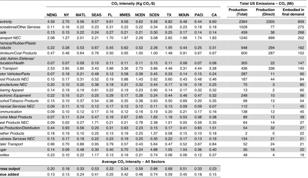
Table 1. Carbon intensity of output by region and sector, ordered by total emissions embodied in final demand.
CO2 Intensity (Kg CO2 /$) Total US Emissions – CO2 (Mt)
NENG NY MATL SEAS FL MWES NCEN SCEN TX MOUN PACI CA
Production (Total) Production (Direct) Embodied in final demand Electricity 4.59 2.70 9.56 9.57 9.61 9.56 9.62 9.58 6.82 6.48 6.44 6.60 2364 2305 809 Recreational/Other Services 0.11 0.16 0.22 0.23 0.31 0.22 0.22 0.34 0.26 0.23 0.18 0.18 1028 77 275 Trade 0.13 0.15 0.22 0.24 0.27 0.21 0.21 0.30 0.25 0.17 0.14 0.14 459 36 268 Transport NEC 2.08 1.27 2.01 2.21 1.70 1.97 2.29 3.08 2.65 1.99 1.74 1.83 1240 899 202 Chemical/Rubber/Plastic Products 0.22 0.28 0.53 0.67 0.45 0.62 0.52 2.26 1.95 0.44 0.25 0.31 948 294 162 Petroleum/Coal Products 0.47 0.46 0.64 0.76 0.50 0.95 1.00 1.00 1.48 0.91 0.67 0.67 600 287 152 Public Admin./Defense/ Education/Health 0.07 0.07 0.09 0.10 0.11 0.11 0.11 0.15 0.11 0.08 0.07 0.06 305 22 147 Air Transport 2.53 2.85 3.85 3.43 3.86 3.36 2.73 3.86 4.46 3.31 4.44 3.28 436 336 145 Motor Vehicles/Parts 0.07 0.18 0.21 0.48 0.12 0.58 0.39 0.45 0.23 0.14 0.15 0.24 287 11 90 Food Products NEC 0.15 0.17 0.31 0.52 0.19 0.88 1.43 0.92 0.60 0.43 0.48 0.46 187 44 84
Manufactures NEC 0.20 0.10 0.20 0.38 0.18 0.31 0.32 0.44 0.17 0.19 0.16 0.25 75 3 80
Wearing Apparel 0.14 0.19 0.19 0.61 0.22 0.19 0.23 0.90 0.14 0.17 0.32 0.32 13 2 60
Electronic Equipment 0.22 0.15 0.21 0.25 0.29 0.17 0.28 0.24 0.44 0.46 0.47 0.32 248 10 56 Alcohol/Tobacco Products 0.15 0.10 0.37 0.54 0.36 0.35 0.38 0.63 0.50 0.69 0.20 0.35 68 13 54 Financial Services NEC 0.09 0.11 0.15 0.12 0.17 0.12 0.12 0.11 0.13 0.09 0.09 0.07 112 1 45
Communication 0.09 0.10 0.12 0.17 0.16 0.12 0.16 0.19 0.20 0.21 0.17 0.16 138 12 45
Bovine Meat Products 0.07 0.11 0.24 0.47 0.16 0.67 2.65 1.62 1.18 0.53 0.38 0.38 89 13 39 Meat Products NEC 0.09 0.02 0.27 1.71 0.21 0.21 0.78 2.38 1.01 0.05 0.59 0.35 64 14 27 Gas Production/Distribution 0.44 0.93 0.56 0.20 0.31 0.63 2.23 0.15 0.17 0.41 0.65 1.51 54 32 27
Leather Products 0.18 0.19 0.10 0.25 0.13 0.19 0.25 1.37 0.08 0.15 0.10 0.18 2 0 22
Business Services NEC 0.15 0.17 0.18 0.22 0.23 0.19 0.25 0.35 0.22 0.17 0.13 0.16 134 21 21
Water Transport 0.96 0.70 0.89 0.95 3.79 0.57 0.43 5.64 0.47 0.52 3.67 0.84 52 24 21
Sugar 0.14 0.09 0.48 0.30 0.40 0.70 5.24 4.88 1.05 1.54 0.36 0.40 30 16 20
Textiles 0.23 0.10 0.22 1.17 0.13 0.19 0.21 0.74 0.06 0.06 0.12 0.37 48 4 19
Average CO2 Intensity – All Sectors
Gross output 0.20 0.18 0.33 0.53 0.33 0.54 0.59 0.86 0.68 0.51 0.33 0.23 Value added 0.13 0.13 0.24 0.41 0.25 0.42 0.46 0.74 0.59 0.45 0.18 0.15
Regional cells report carbon intensity measured as tons of CO2 per dollar of output in each region. CO2 intensity includes emissions embodied in intermediate inputs.
11
The final three columns of Table 1 display measures for the total nation-wide emissions associated with each sector, in Mt CO2. The first of these columns displays the total emissions embodied in each sector’s output, both directly (in the production of that sector) and indirectly (through intermediates, including electricity). The second-to-last column displays the amount of CO2 directly emitted in the production of each sector7. For example, in the Electricity sector, almost all emissions are direct production emissions—2305 Mt out of the total 2364 Mt. For many sectors, however, a large share of emissions is embodied in intermediate inputs. Very little carbon (77 Mt) is emitted directly in the production of the Recreational/Other Services sector, but its output is associated with a large amount of emissions (1028 Mt) when embodied emissions are included (as Recreational/Other Services requires electricity, construction, transportation, and other emissions-intensive inputs). The last column displays the total amount of emissions embodied in the final demand of each sector. The Electricity sector constitutes the largest contributor to emissions in final demand, but again we see that sectors with cleaner production (e.g., Recreational/Other Services, Trade) also contribute significantly to final demand emissions. This metric incorporates emissions that occurred outside of the US; the difference between total direct production emissions (summed across sectors) and those embodied in final demand is due to emissions embodied in international imports and exports. In some sectors, a large share of emissions embodied in final demand is imported—the consumption of Wearing Apparel, for example, is responsible for 60 Mt of CO2 even though US production of Wearing Apparel is only responsible for 13 Mt. Also, we can see that some sectors associated with large production
emissions, such as Chemical/Rubber/Plastic Products, are not responsible for the same proportion of final demand emissions.
The last two rows of Table 1 illustrate how differences in each sector’s CO2 intensity and each region’s composition of production relate to differences in the average CO2 intensity of regional production. The first of these rows displays the CO2 intensity of gross output, and corresponds to the average of the sector-level intensities above it, weighted by gross output in that region. These values reveal very large differences between regions, ranging from an average of 0.18 kg CO2/$ of output for New York, to an average of 0.86 kg CO2/$ for the South Central region. This measure encompasses all emissions associated with production in a region (production emissions and emissions embodied in intermediates). The last row of Table 1 shows emissions from
production in the region itself as the CO2 intensity of value added in each region (defined as the amount of CO2 emitted directly in the production of all sectors, divided by value added – or GDP – in that region). We divide by value added rather than the gross value of output, relating
in-region emissions to in-region economic activity. These values vary even more across regions than the gross output estimate, as the traded intermediates included in the gross output measure mitigate differences in direct CO2 intensity between regions.
7 The sum of these emissions over all sectors is 5309 Mt. This number does not include emissions occurring in final demand. According to the EPA GHG inventory, CO2 emissions from fossil fuel combustion corresponded to 5753 Mt in 2005, 358 Mt of which were residential emissions.
12
3.1 Regional Emissions and Consumption-Based Emissions
Before switching our focus to measuring the CO2 intensity of consumption, we find it
informative to use our MRIO framework to construct regional CO2 inventories. We compute
these both from a production and a consumption perspective, allowing for a differential
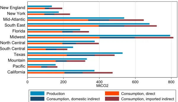
attribution of responsibility for emissions across regions. Figure 3 displays regional production-
and consumption-based estimates of CO2 emissions. The top bar corresponds to production-based
emissions, including all CO2 emitted within the region, both in production and final demand. The bottom bar corresponds to consumption-based emissions, distinguishing between sources of emissions. Consumption-based emissions are computed using the MRIO framework, which tracks emissions through the production chain to final consumption; these calculations include not only the carbon emitted in the production of final goods consumed in the region, but also the CO2 emitted anywhere in the production of goods used as intermediates for all goods which are ultimately consumed in the region.
Figure 3. CO2 accounting of consumption, compared to regional production emissions. Both the production- and consumption-based calculations include direct consumption emissions (e.g., Midwest values include CO2 emitted as households consume fossil fuels and electricity) as well as domestic indirect consumption emissions (e.g., Midwest values include CO2 emitted during the production of cars in the Midwest that were then purchased in the Midwest). However, the two metrics differ in terms of the CO2 embodied in trade. Production estimates include the carbon emitted during the production of goods and services that are
ultimately consumed outside of the region (e.g., Midwest production values include CO2 emitted to produce glass in the Midwest for cars produced in the Midwest that were ultimately purchased in New York), while consumption estimates include imported indirect emissions – CO2 emitted during production outside of the region, imported as an intermediate input or final good (e.g.,
0 200 400 600 800 MtCO2 California Pacific Mountain Texas South Central North Central Midwest Florida South East Mid-Atlantic New York New England
Production Consumption, direct
13
New York consumption values include CO2 emitted to produce glass in the Midwest for cars that were ultimately purchased in New York).
Comparison of the top and bottom bars in Figure 3 reveals whether a region is a net importer or a net exporter of CO2. We find that the New England, New York, Mid-Atlantic, Florida and California regions are all significant net importers of embodied carbon. The Southeast, Midwest, North Central and Pacific regions are nearly balanced with imports of carbon very close to exports. The South Central, Mountain and Texas regions are exporters of carbon. These statistics include carbon imported or exported abroad and so do not net to zero for the US as a whole (which is overall a net importer of embodied carbon).
Neither the production-based nor consumption-based estimates displayed in Figure 3 include “re-exports” of CO2—the emissions embodied in a region’s imports of goods which are then transformed and ultimately exported to be consumed outside of the region. These emissions are not attributed either to domestic consumption nor production, but the MRIO framework allows us to compute re-exports and we note that they comprise a relatively large share of CO2 trade in most regions—46% of total carbon exports (both domestically emitted and imported), with a maximum of 76% in New England, and 36% of total imports (both domestically consumed and re-exported), with a maximum of 46% for the Midwest.8
Figure 3 highlights the extent to which measures of CO2 can differ when computed on consumption rather than a production basis. Consider California, for example: its
consumption-based emissions are about 100 Mt larger than its production-based emissions; California imports 1.85 times more embodied CO2 than it exports. Although we do not trace emissions over time in this analysis, this difference suggests reason for caution about drawing policy conclusions from curves such as the Rosenfeld Curve, which shows a marked decline in California’s per capita energy consumption from 1963–2009 (Rosenfeld and Poskanzer, 2009), but may largely underestimate the amount of emissions for which the state is responsible. The decline of emissions observed over time in California may be partially attributed to the state importing more of the emissions embodied in its consumption; however, without an evaluation similar to ours that goes back over time, one cannot conclude whether California has reduced emissions relatively well compared to other parts of the country, or whether emissions have simply shifted out of the state for various economic or regulatory reasons. Similar to California, both New England and New York import large shares of the emissions for which they are responsible. Overall, Figure 3 highlights the importance of tracking trade flows: almost all regions consume more imported CO2 (imported indirect) than domestically emitted CO2
(domestic indirect), and most regions export a majority of the CO2 they emit in the production of goods.
8 To illustrate the role of bilateral trade flows in generating these estimates, Table D1 (Appendix D) displays the CO2 embodied in bilateral trade flows (in Mt CO2) of US regions, between regions as well as with their major international trading partners.
14
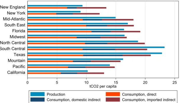
Figure 4. CO2 emissions per capita (tonnes)
Figure 3 does not account for differences in region sizes. In Figure 4, we normalize the values by each region’s population. Shifting to per capita emissions measurements, two things stand out. First, the ranking of regions changes significantly: Midwest emissions—formerly the highest by both measures—are lowered; South Central moves from the middle of the list to become the region with the highest production emissions per capita, whereas Texas has the highest consumption emissions per capita; New York has both the lowest production- and
consumption-based emissions, replacing New England and Pacific, respectively; and California, even with its substantial imported emissions, remains among the lower-emitting regions. Second, although accounting for size differences causes the variation in emissions to drop significantly, it is still quite large—particularly when measured on a production basis. The ratio of highest to lowest production emissions per capita is still roughly two to one—a considerable amount, especially since we display results at a relatively high level of aggregation. The variation in consumption emissions per capita is lower, as trade between regions partially equalizes emission rates; however, large differences remain between regions’ per capita consumption of CO2.
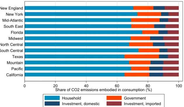
3.2 Consumption: Household, Government and Investment Final Demand
As described in Section 2, we use a broad definition of consumption, attributing to regions not only the emissions associated with household demand, but also government and investment demand. Figure 5 shows the total CO2 content of consumption as in Equation (13), displaying the percentages of final demand types for each region. Private household demand dominates, but government and investment demand account for non-negligible shares of consumption emissions. On average, household final demand accounts for 70% of emissions, government demand for 15%, domestic investment (emissions embodied in domestic investment that are attributed to domestic consumption) for 7% and imported investment (emissions embodied in out-of-region
0 5 10 15 20 25
tCO2 per capita
California Pacific Mountain Texas South Central North Central Midwest Florida South East Mid-Atlantic New York New England
Production Consumption, direct
15
investment that is attributed to domestic consumption) for 8%. Overlooking investment-related consumption emissions would therefore lead to a substantial underestimation of the emissions embodied in final demand.
Figure 5. Percentage of each final demand type for consumption emissions, by region. 3.3 The Direct and Indirect CO2 Intensity of Consumption
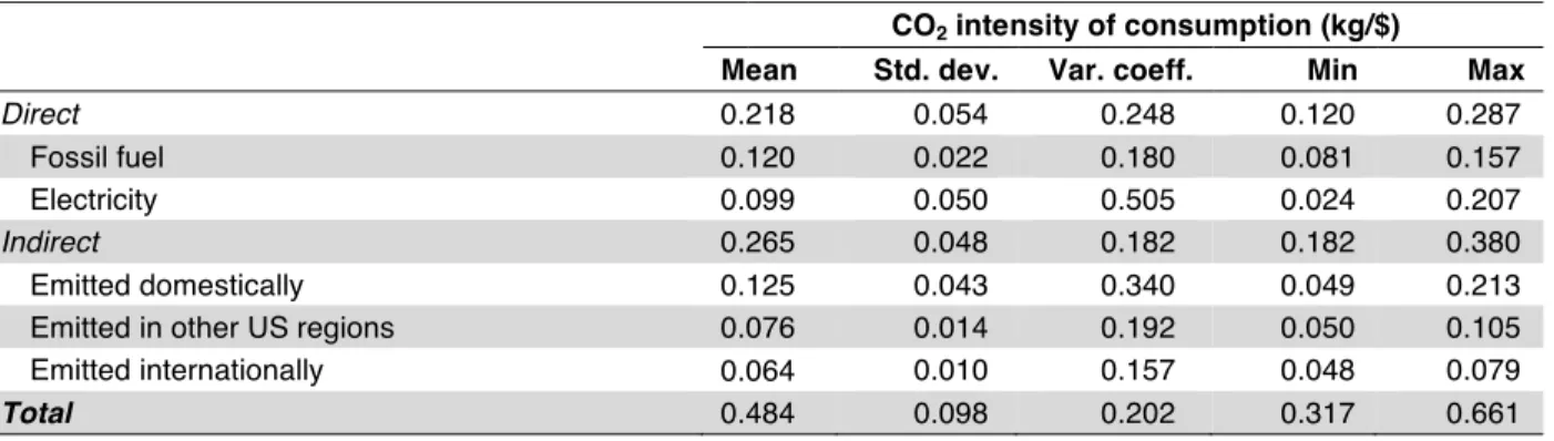
Figure 6 displays the average CO2 content per dollar—or CO2 intensity—of consumption for each region. Indirect-only CO2 content is shown in red, while total CO2 content is shown in blue. The difference between the two bars corresponds to the final demand of emissions by
consumption of fossil fuels and electricity by households, government and investing firms. Table 2 provides summary statistics on these intensity measures, weighted by total consumption in each region such that the mean value corresponds to the US mean value. Table A1 (see Appendix A) displays calculations of this intensity for each individual US state.
In Figure 6, we observe that the indirect component of consumption accounts for more than half of the total intensity. On average over the whole country, each dollar of consumption contains 0.218 kg of direct emissions and 0.265 kg of indirect emissions. While policy makers tend to focus on the impact of carbon pricing on energy goods that cause direct emissions through consumption (e.g., gasoline, home heating fuels and electricity), most consumer spending is on non-energy goods where embodied emissions occurred during production. Even though non-energy goods and services have low emissions intensities relative to that of energy goods, non-energy emissions amount to a large share of consumption emissions because such a large portion of the household budget is spent on these goods. One implication, then, is that while the impact of carbon pricing might be most obviously seen in the price of energy goods, the budget may also be impacted by the accumulation of very small, individually unremarkable increases in the cost of all other goods.
0 20 40 60 80 100
Share of CO2 emissions embodied in consumption (%) California Pacific Mountain Texas South Central North Central Midwest Florida South East Mid-Atlantic New York New England Household Government
16
Figure 6. Total vs. indirect-only CO2 consumption intensity. Table 2. CO2 intensity of consumption – Summary statistics across US regions.
CO2 intensity of consumption (kg/$)
Mean Std. dev. Var. coeff. Min Max
Direct 0.218 0.054 0.248 0.120 0.287
Fossil fuel 0.120 0.022 0.180 0.081 0.157
Electricity 0.099 0.050 0.505 0.024 0.207
Indirect 0.265 0.048 0.182 0.182 0.380 Emitted domestically 0.125 0.043 0.340 0.049 0.213 Emitted in other US regions 0.076 0.014 0.192 0.050 0.105 Emitted internationally 0.064 0.010 0.157 0.048 0.079
Total 0.484 0.098 0.202 0.317 0.661
CO2 intensity defined as the physical quantity of CO2 in kg per dollar value of consumption; all values weighted by
total regional consumption; Variation coefficient corresponds to the standard deviation divided by the mean.
Both direct and indirect emissions vary across regions; however, the direct emissions intensity of consumption ranges from just 0.12–0.29 kg/$ (generally, northern states have greater fossil fuel requirements for heating, and southern states have greater electricity requirements for air conditioning). Overall, the range of direct intensities is roughly consistent with that found by Hassett et al. (2009) and Mathur and Morris (2012). The picture changes, however, when we focus on indirect emissions. These are found to vary considerably more than suggested by the aforementioned studies, which argued that the variance in geographic distribution of indirect emissions is much lower than that of direct emissions. We find that indirect carbon intensity varies from 0.18–0.33 kg/$—a ratio of almost two to one. In contrast, Mathur and Morris (2012) find that the CO2 intensity of the most emissions-intense region is less than 25% higher than that of the least intense region, and that direct emissions vary twice as much between regions as indirect emissions. While direct comparison is difficult due to slight differences in regional
0 .1 .2 .3 .4 .5 .6 .7
CO2 intensity of consumption (kg/$)
California Pacific Mountain Texas South Central North Central Midwest Florida South East Mid-Atlantic New York New England
17
aggregation relative to Mathur and Morris (2012)9, there is clearly considerably more variation in the indirect emissions statistics computed using MRIO. There are also differences in the relative magnitudes of the measures across regions; however, given the aforementioned issue of regional composition, it is difficult to draw substantive conclusions from these variations.
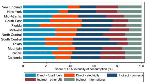
Figure 7. Composition of CO2 intensity of consumption, by US region.
Figure 7 illustrates the locus of emission for the carbon embodied in consumption, displaying the composition of emissions in each region. Emissions are categorized as direct, if stemming from the combustion of fossil fuels in final demand (Direct – fossil fuels) or from the final
demand for electricity (Direct – electricity), or indirect, if having occurred within region (Indirect – domestic), in other regions of the US (Indirect – other US), or internationally (Indirect –
international). Figure 7 suggests that most indirect emissions are non-domestic: domestically emitted indirect emissions correspond to just 0.13 kg/$ of consumption on average, while imported emissions account for 0.14 kg/$ of consumption on average, with nearly half of that (0.06 kg/$) coming from international sources. There is slightly less variation in Indirect – international intensity than in Indirect – other US intensity, indicating that the importance and composition of international imports varies less from region to region than domestic imports. The large differences in the indirect CO2 intensity of consumption revealed by Figure 7 have an important implication regarding the incidence of carbon taxation: the extent to which
households will be affected will vary across regions, not only because of differences in the consumption of fossil fuels and electricity, but because of differences in non-energy consumption as well. These differences may be caused by differences in consumption patterns; alternatively, households might consume similar sets of goods purchased from different sources (thus
9 Figure A1 (Appendix A) reproduces the direct and indirect burdens of a carbon tax as estimated in Table 7 of Mathur and Morris (2012). These are theoretically equivalent to the CO2 content of consumption.
0 20 40 60 80 100
Share of CO2 intensity of consumption (%)
California Pacific Mountain Texas South Central North Central Midwest Florida South East Mid-Atlantic New York New England
Direct - fossil fuels Direct - electricity Indirect - domestic Indirect - other US Indirect - international
18
embodying different amounts of carbon). To better understand the source of this variability, we
compare the CO2 consumption emissions computed using a full MRIO dataset to those computed
using average US intensities for non-energy goods (e.g., Hassett et al., 2009).
3.4 Understanding the Source of Differences in CO2 Intensity of Consumption
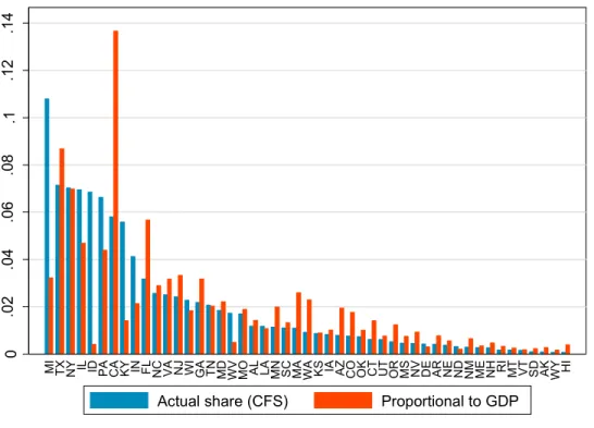
As noted earlier, a key assumption made by recent studies (e.g., Hassett et al., 2009) is that commodities produced in and exported out of any given state are equally likely to be consumed in any other given state; however, our results suggest that this homogeneity assumption may drive the result that indirect emissions are nearly constant (as a share of income) in those studies. To illustrate this, Figure 8 indicates the proportion of exports from Ohio going to each other state. It displays both actual shares from the 2007 Commodity Flow Survey10—the source of bilateral trade data in our dataset—and the shares that would be implied by uniform sourcing (based solely on the importing state’s share of GDP).
Figure 8. Share of exports from Ohio, by destination state.
Our results suggest that—similar to what would be predicted by a gravity model—trade depends not only on the importing state’s size, but also on geographical proximity. Exports from Ohio to neighboring Michigan are much larger than its GDP would suggest, whereas exports to distant California are much lower. The Commodity Flow Survey may be capturing flows of goods which are further transported without transformation (e.g., for warehousing) and may thus exaggerate the effect of distance on trade; however, trade shares clearly depend on geographical proximity, and trade costs—including transport costs—play a role in limiting trade. Thus, the
10 Available online at http://www.census.gov/econ/cfs/.
0 .0 2 .0 4 .0 6 .0 8 .1 .1 2 .1 4 S ha re o f e xp or ts f ro m O hio MI TX NY IL ID PA CA KY IN FL NC VA NJ WI GA TN MD WV MO AL LA MN SC MA WA KS IA AZ CO OK CT UT OR MS NV DE AR NE ND NM ME NH RI MT VT SD AK WY HI Actual share (CFS) Proportional to GDP
19
regional differences in production CO2 intensities (identified in Table 1) can lead to differences in the overall CO2 intensity of consumed goods across states.
To quantify the effect of these differences and make a direct comparison with the method used in Hassett et al. (2009) and Mathur and Morris (2012)—which we will refer to as the HMM method—we calculate CO2 intensities while applying their simplifying assumptions to our data and regional aggregation. Recall that we use region-specific estimates of the input-output matrices Ar and CO2 intensity vectors Fr. To determine the sources of variability for indirect emissions, we re-compute consumption emissions under four different sets of assumptions (using average national values of A and F) and compare these results to our original MRIO calculations. The four sets of assumptions are as follows:
• US AVG – We use average US intensities for domestic production and imports in all
regions. All cross-regional variation is explained by differences in consumption shares, as technological differences or differences in the within-sector composition of consumption are assumed away. Theoretically, we would apply these assumptions only if our data were limited to average US production intensity data (i.e. only a national I-O table), or if region-specific I-O tables were only available without an intra-national bilateral trade matrix (rendering us unable to compute region-specific indirect embodied emissions). • US AVG INDIRECT (HMM) – As in Hassett et al. (2009) and Mathur and Morris (2012),
we assume US average CO2 intensities for non-energy goods, but use region-specific values for direct emissions (including electricity). Theoretically, we would apply these assumptions if, in addition to the US AVG data, we knew cross-regional differences in the emissions intensity of fossil fuels and electricity only.
• US AVG INDIRECT + INT IMP – Domestic emissions are computed as above, but we use
observed average US emission intensities for international imports. Theoretically, we would apply these assumptions if, in addition to the US AVG INDIRECT data, we had bilateral international trade data linked to foreign production intensity data, but without the exact sourcing of imports by sub-national region.
• AVG INT IMP – This set of assumptions uses the intra-national bilateral trade data to
compute indirect intensities of all goods, accounting for differences in domestic sourcing, but uses US average intensities for international imports. Theoretically, we would apply these assumptions if we had all the data necessary for MRIO analysis within the US, but without international import data.
In all cases, the direct emissions from household fossil fuel use will be identical. A more detailed algebraic description of each of these assumptions can be found in Appendix C.
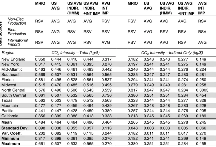
Table 3 displays, for all regions, the CO2 intensity of consumption for each of the above groups compared to the full MRIO estimates. The left side of the table shows the total values encompassing both direct and indirect consumption of CO2. The right side shows values for the indirect intensity only—this is where we expect differences across assumptions to be larger. The last five rows of Table 3 describe the distribution of intensities under each set of assumptions.
20
Table 3. CO2 intensity of consumption results: comparing MRIO results to assumption sets. MRIO US AVG US AVG INDIR. (HMM) US AVG INDIR. +INT IMP AVG INT IMP MRIO US AVG US AVG INDIR. (HMM) US AVG INDIR. +INT IMP AVG INT IMP Dat a S o u rc e
s Non-Elec. Production RSV AVG AVG AVG RSV RSV AVG AVG AVG RSV
Elec.
Production RSV AVG RSV RSV RSV RSV AVG RSV RSV RSV International
Imports RSV AVG AVG RSV AVG RSV AVG AVG RSV AVG Region CO2 Intensity—Total (kg/$) CO2 Intensity—Indirect Only (kg/$)
New England 0.350 0.444 0.410 0.444 0.317 0.182 0.243 0.243 0.277 0.149 New York 0.317 0.415 0.361 0.395 0.270 0.197 0.241 0.241 0.275 0.149 Mid-Atlantic 0.463 0.446 0.461 0.493 0.442 0.246 0.244 0.244 0.276 0.224 Southeast 0.569 0.507 0.531 0.564 0.565 0.285 0.247 0.247 0.280 0.281 Florida 0.581 0.495 0.528 0.561 0.537 0.294 0.241 0.241 0.274 0.250 Midwest 0.515 0.470 0.485 0.516 0.495 0.279 0.249 0.249 0.281 0.258 North Central 0.576 0.490 0.506 0.543 0.559 0.317 0.247 0.247 0.284 0.3003 South Central 0.661 0.507 0.532 0.565 0.736 0.380 0.251 0.251 0.284 0.454 Texas 0.562 0.503 0.479 0.512 0.563 0.328 0.244 0.244 0.277 0.328 Mountain 0.477 0.477 0.459 0.494 0.439 0.267 0.248 0.248 0.283 0.228 Pacific 0.441 0.447 0.428 0.459 0.389 0.257 0.244 0.244 0.276 0.205 California 0.356 0.399 0.388 0.413 0.333 0.213 0.245 0.245 0.269 0.189 Mean 0.484 0.464 0.464 0.496 0.464 0.265 0.245 0.245 0.278 0.245 Standard Dev. 0.098 0.038 0.055 0.057 0.113 0.048 0.003 0.003 0.005 0.066 Var. Coeff. 0.202 0.082 0.119 0.115 0.244 0.182 0.011 0.011 0.017 0.270 Minimum 0.317 0.399 0.361 0.395 0.270 0.182 0.241 0.241 0.269 0.149 Maximum 0.661 0.507 0.532 0.565 0.270 0.380 0.251 0.251 0.284 0.455 Data sources are RSV (Region-Specific Values) and AVG (Average US values). CO2 intensity measured in kg/$ of
consumption. Note that for Indirect Only results, US AVG and US AVG INDIR. generate the same values.
As seen in the last five rows, the restrictive assumptions of US AVG lead to intensity values that are, on average, lower than MRIO results (average of 0.46 instead of 0.48 kg/$). This difference indicates that internationally imported goods are more CO2 intensive than domestic goods on average—and, more importantly, that they also have dramatically lower variance. The coefficient of variation (standard deviation standardized by the mean) of indirect emissions in this case is only 0.01 – much less than the 0.18 found using MRIO. For overall consumption-based emissions, this translates to a variation coefficient of less than half of what is found under MRIO.
These numbers indicate that variations in consumption patterns explain only a small part of the regional disparities in the average CO2 content of consumption, most of which is explained by
differences in technology and production intensities. Under the US AVG INDIRECT (HMM)
assumptions, the coefficient of variation increases slightly, from 0.08 kg/$ to 0.12 kg/$, but
nonetheless it remains much lower than under MRIO. Under US AVG INDIRECT+INT IMP, we
identify the importance of accounting for the CO2 intensity of international imports: these assumptions increase the mean intensity of US consumption, as goods imported from foreign sources have higher intensities on average, but they do not affect variability across regions. Finally, AVG INT IMP shows the importance of accounting for international trade flows. These values closely resemble MRIO results, although the mean is lower.
21
3.5 Importance of Accounting for International and Sub-National Trade Flows From a practical standpoint, the most important aspect to consider when comparing
methodologies might be the precision of estimates for particular regions that policy makers may care about. To investigate this, we also express differences in methodologies by computing the difference in carbon estimates relative to MRIO estimates. These differences are measured as 100 × (counterfactual estimate / MRIO estimate -1). Table 4 summarizes the median and maximum differences found under each set of assumptions. The maximum is computed both across the 12 aggregated regions (remaining comparable with Hassett et al. (2009) and Mathur and Morris (2012) who work at a similar level of aggregation), and across all 50 states.
Table 4. Median and maximum differences in CO2 intensity of consumption across assumptions (in %).
Total Indirect only
Median Max (regions) Max (states) Median Max (regions) Max (states)
US AVG 11.47 31.06 53.84 16.69 34.01 69.45
HMM - US AVG INDIRECT 9.14 19.55 51.43 16.69 34.01 69.45 US AVG INDIRECT+INT IMP 6.08 27.02 47.05 11.25 51.84 63.53 AVG INT IMP 5.98 12.24 24.39 10.95 19.70 32.93
Figure 9. Difference between the HMM methodology and MRIO
Differences between the estimates generated using the assumptions in US AVG INDIRECT
(HMM) and those generated using MRIO are shown in Figure 9 for both total and indirect
emissions. Estimates of these differences for all 50 states are shown in Table A1 (see Appendix A). Over all states, the median absolute difference for indirect emissions is 17%; however, the error arising from not accounting for differences in the carbon intensity of trade flows is much higher in
particular states. In the most extreme cases, the assumptions in US AVG INDIRECT (HMM)
22
simultaneously underestimating that of households in North Dakota by about 70%. This translates to a median difference of 11% for the total CO2 intensity of consumption, which can be as large as 53% for certain states.
Figure 9 shows that, even after adding true international import intensities to the assumptions of HMM (as in the US AVG INDIRECT+INT IMP assumption), the median difference is still 14% This implies that the main source of error is the assumption of homogeneous production patterns across regions of the US. Correct treatment of international import intensities does matter, though, and ignoring them (as in the AVG INT IMP assumption) yields smaller but still non-negligible errors. 4. CONCLUSIONS
We have used a multi-regional input-output (MRIO) model to understand the production and consumption patterns of CO2 in the US. Our first significant finding is that state level
responsibility for emissions differs substantially when emissions are allocated on a production basis rather than a consumption basis. For example, California’s per capita emissions are much higher when allocated on a consumption basis, due to the large net inflow of emissions embodied in the goods it imports.
Our second finding is that there is significant regional heterogeneity in emissions per dollar of consumption, even when focused on the carbon embodied in non-energy consumption. This result contrasts sharply with previous studies. We find that differences in consumption patterns do not explain a large part of the heterogeneity, and that it may be better explained by differences in production intensities, and the sourcing of domestic and international imports. The patterns of bilateral trade between regions are such that differences in the CO2 intensity of production across regions are reflected in CO2 intensities of consumption. Thus, we conclude that the assumption of
homogeneity made by previous studies has lead to underestimation of differences in CO2
consumption intensity across states. We find good reason to believe that disparities in the impact of carbon pricing go well beyond direct energy consumption and should be taken into account.
Our results are important for understanding regional patterns of CO2 intensity in consumption. They may thus contribute to explaining regional variation in support for climate policy in the United States. Our findings are also relevant for analysis of state-level carbon policy; given the failure to enact carbon pricing at the national level, sub-national policy is becoming increasingly relevant. Carbon intensity of production and consumption in different sub-national regions could help determine the likelihood of enacting policy in those regions, as well as inform the design of that policy—including, for example, whether carbon pricing should be enacted on an upstream (production) or a downstream (consumption) basis.
5. REFERENCES
Caron, J. and S. Rausch, 2013: A Global General Equilibrium Model with US State-Level Detail for Trade and Environmental Policy Analysis -- Technical Notes, Cambridge, MA: MIT Joint Program on the Science and Policy of Global Change, Joint Program Technical Note 13.
Davis, S.J. and K. Caldeira, 2010: Consumption-based accounting of CO2