HAL Id: hal-01191540
https://hal.archives-ouvertes.fr/hal-01191540
Submitted on 2 Sep 2015
HAL is a multi-disciplinary open access
archive for the deposit and dissemination of
sci-entific research documents, whether they are
pub-lished or not. The documents may come from
teaching and research institutions in France or
abroad, or from public or private research centers.
L’archive ouverte pluridisciplinaire HAL, est
destinée au dépôt et à la diffusion de documents
scientifiques de niveau recherche, publiés ou non,
émanant des établissements d’enseignement et de
recherche français ou étrangers, des laboratoires
publics ou privés.
A sub-Riemannian modular approach for diffeomorphic
deformations
Barbara Gris, Stanley Durrleman, Alain Trouvé
To cite this version:
Barbara Gris, Stanley Durrleman, Alain Trouvé. A sub-Riemannian modular approach for
diffeo-morphic deformations. 2nd conference on Geometric Science of Information, Oct 2015, Paris-Saclay,
France. �hal-01191540�
A sub-Riemannian modular approach for
diffeomorphic deformations
Barbara Gris1,2, Stanley Durrleman2, and Alain Trouvé1
1 CMLA, UMR 8536, École normale supérieure de Cachan, France 2
Inria Paris-Rocquencourt, Sorbonne Universités, UPMC Univ Paris 06 UMR S1127, Inserm U1127, CNRS UMR 7225, ICM, F-75013, Paris, France
Abstract. We develop a generic framework to build large deformations from a combination of base modules. These modules constitute a dy-namical dictionary to describe transformations. The method, built on a coherent sub-Riemannian framework, defines a metric on modular de-formations and characterises optimal dede-formations as geodesics for this metric. We will present a generic way to build local affine transformations as deformation modules, and display examples.
1
Introduction
A central aspect of Computational Anatomy is the comparison of different shapes, which are encoded as meshes or images. A common approach is the study of deformations matching one shape onto another, so that the differences between the two shapes are encoded by the deformation parameters [9, 11, 17]. In order to study differences between subjects on a particular structure, it should be useful to constrain locally the deformation, to favour realistic anatomic deforma-tions, or to introduce some anatomical priors. For instance, for cortical surfaces with different sulci topography, one can prefer to favour lateral displacement over the creation of new sulci. Large deformations are commonly obtained through the integration of a vector field [4, 10, 13, 18] and a natural route is to intro-duce the constraints in the vector fields instead of the final diffeomorphism [19]. The vector field could be restricted, via a finite dimensional control variable, to a state dependent finite dimensional subspace generated by a finite basis and conceptualized in structures called hereafter deformation modules. Deformation modules should create interpretable deformations, and several modules should be allowed to combine to form more complex compound deformation modules in the spirit of Grenander’s Pattern Theory [7].
Preliminary instantiations of the concept of deformation modules can be found in several early works. In the poly-affine framework [3, 14, 20], deforma-tions are created by the integration of a poly-affine stationary vector field. This vector field is a sum of few local affine transformations, which are then easily interpretable and share some features of deformation modules even if regions of each affine component are not updated during the deformation. In the LDDMM framework, a Riemannian structure is defined on the group of diffeomorphisms
and optimal matchings are geodesics for this metric [2, 10]. Several discretization schemes based on landmarks induce examples of finite dimensional state depen-dent representations of the velocity fields updated along the deformation and could be rephrased inside our definition of deformation modules. Note that the discretization scheme are thought of as approximations of the unconstrained non-parametrized infinite dimensional case. In a recently developed sparse-LDDMM framework [6, 12, 15], the vector field is constrained to be a sum of a fixed num-ber of local translations, carried by control points, with a more clearer focus on finite-dimensionality and local interpretability. Extension to locally more com-plex transformation are considered in [8, 16].
However, a consistent and general mathematical framework able to handle a large body of modular based large deformations is still missing in computa-tional anatomy. A useful theory should not only provide a clear definition of deformation modules, but also explains how a hierarchy of deformation modules can be induced from basic one and how a Riemannian (or sub-Riemannian) set-ting can be defined underlying the computation of optimal large deformations and organizing the action of the different modules in the deformation process. This paper is a first attempt in that direction and presents a mathematical and computational sub-Riemannian framework to build large deformations from well defined deformation modules.
We will present several instances of deformation modules generating multi-scale and locally affine vector fields as simple illustrative examples. We will show trajectories that can be built from the combination of such modules, and how the component of a particular module can be recovered and followed through the integration.
2
Definition of a deformation module
Intuitively, a deformation module creates a vector field parametrized in low di-mension, describing a distinctive aspect of a larger deformation pattern. This notion should embrace at least the notion a sum of local translations, scal-ings or other local affine transformations as simple examples. In the following, C1
0(Rd) will be the set on C1continuous mapping v vanishing at infinity equipped with the usual supremum norm on v and its first derivative, and Diff10(Rd) the open subset of Id + C01(Rd) of C1diffeomorphisms. We recall that for any curve v ∈ L1 = L. 1([0, 1], C01(Rd)) there exists a unique curve t 7→ φvt ∈ Diff
1 0(Rd) solution of the flow equation ˙φvt = vt◦ φvt, with φv0= id.
Let O be a finite dimensional manifold and (φ, o) 7→ φ.o a C1 action of Diff10(Rd) on O in the sense that (φ, o) 7→ φ.o is continuous and there exists a continuous mapping ξ : O × C01(Rd) → T O called the infinitesimal action, so that v 7→ ξo(v) = ξ(o, v) is linear continous, o 7→ ξo. is locally Lipschitz and for any v ∈ L1, the curve t 7→ ot= φ. vt.o0is absolutly continuous (a.c.) and satisfies
˙ot= ξot(vt) for almost every t ∈ [0, 1].
Definition 1 (Deformation module). We say that M = (O, H, V, ζ, ξ, c) is a deformation module with geometrical descriptors in O, controls in H, infinitesi-mal action ξ, field generator ζ and cost c if H is a finite dimensional Euclidean space, V is an Hilbert space with V C
0
,→ C1
0(Rd), ζ : O × H → O × V is a con-tinuous mapping such that h 7→ ζo(h) is linear where ζ(o, v) = (o, ζo(v)), o 7→ ζo is locally Lipschitz and c : O × H → R+ is a continuous mapping such that h 7→ co(h) = c(o, h) is a positive quadratic form on H and there exists C > 0. such that for each o, h:
|ζo(h)|2V ≤ Cco(h) . (1) Let us explain how a deformation modules induces large deformations. Definition 2 (Finite energy controled paths on O). Let a, b ∈ O. We denote Ωa,b the set of mesurable curves t 7→ (ot, ht) ∈ O × H where ot is a.c., starting from a and ending at b, such that ˙ot = ξot(vt) for vt= ζo. t(ht) and E(o, h)=. R1
0 cot(ht)dt < ∞ where E(o, h) is called the energy of (o, h).
Thanks to (1) and the smoothness condition for deformation modules one get the following construction of flows :
Proposition 1 (Flows generated by a deformation module). Let (o, h) ∈ Ωa,b and v = ζo(h). ThenR1
0 |vt| 2 Vdt ≤ C R1 0 cot(ht)dt < ∞ so that v ∈ L 2([0, 1], V ) ⊂ L1 and ot= φvt.o0. Moreover, R01|ht|2
Hdt ≤ (suptkc−1ot k) R1 0 cot(ht)dt < ∞ (with kc−1 o k .
= sup|h|H=1co(h)−1) so that h ∈ L2([0, 1], H).
A more geometrical point of view on deformation modules would be to iden-tify ζ (resp. ξ) as a continuous morphisms between the two vector bundles O × H and O × V (resp. O × V → T O) and c as a metric on O × H. Now, ρ = ξ ◦ ζ : O × H → T O and c induce a sub-Riemannian structure on O. (as defined in [1]). Moreover, indexed by the choice of a ∈ O, we can induce a sub-Riemannian structure on Diff10(Rd) by considering ρa : Diff10(Rd) × H → T Diff10(Rd) = C01(Rd) such that ρaφ(h)
.
= ζφ.a(h) and the metric on Diff10(Rd)×H given by caφ(h)= cφ.a(h)..
During the trajectory, the geometrical descriptor ot creates the vector field ζo(h) which acts back on otthrough the infinitesimal action ξ. Then, as explained in figure 1, ξ can be seen as a feedback action, allowing geometrical descriptors to evolve with the vector field.
2.1 First example : sum of local translations
This first example explains how the construction of [6] can be seen as a de-formation module. Let σ ∈ R+
, and D ∈ N, we want to build a module M that would generate a sum of D local translations acting at scale σ. We set O = (Rd)D (families of D points), H = (Rd)D (families of D vectors) and V = Vσ the scalar Gaussian RKHS of scale σ. For o = (zi) ∈ O, we define ζo: h = (αi) ∈ H 7→PDi=1Kσ(zi, ·)αi, ξo: v ∈ V 7→ (v(zi))i (application of the vector field at each point) and co: h = (αi) ∈ H 7→ |P
iKσ(zi, ·)αi| 2 Vσ.
Fig. 1. Schematic view of a deformation module.
Fig. 2. Schematic view of a combination of deformation modules.
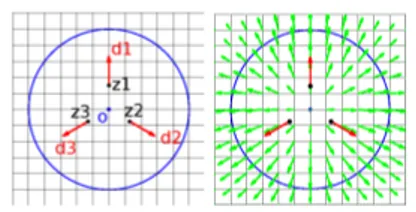
Fig. 3. Local scaling. Left : Geometri-cal descriptor o (in blue) and intermedi-ate tools (in black and red). Right: Plot of the resulting vector field in green.
Fig. 4. Local rotation. Left : Geometri-cal descriptor o (in blue) and intermedi-ate tools (in black and red). Right: Plot of the resulting vector field in green.
2.2 Second example : constrained local affine transformations
We present here a generic way to build a particular kind of local affine trans-formation as a detrans-formation module. Let us first start by an illustrative example of a local scaling in dimension 2 parametrized by a scale σ, a center o and a scaling ratio h. From σ and o, we build 3 points zj and 3 unit vectors dj as described in Figure 3. We can then define the vector field generated by the geo-metrical descriptor o and the control h by ζo(h)=. P3j=1Kσ(zj(o, σ), ·)dj(o, σ)h. We emphasize here that points zj and vectors dj are intermediate tools used to build the vector field but that the latter is only parametrized by σ, o and h. We can then define the module M by the following spaces :V = Vσ, O = Rd, H = R and applications, for o ∈ O: ζo, ξo : v ∈ C0(R1 d) 7→ 13
P3 j=1v(zj(o, σ)) and co: h ∈ H 7→ |ζo(h)|2 Vσ = P j,j0Kσ(zj, zj0)dTjdj0h2.
If we change the rule to build vectors dj, we can build a local rotation, see Figure 4. More generally, we can set any kind of rules to build points zj and unit vectors dj from a geometrical descriptor o to create another type of local transformation. We have here defined a generic way to build a module that gen-erates a vector field based on user’s assumptions. It is the way to incorporate anatomical prior in the deformation.
2.3 Third example : unconstrained local affine transformations Some more complex local affine transformations can be needed. Any local affine deformation in dimension d can be approximated by a sum of d + 1 local transla-tions carried by points close to each other with respect to the scale. In this spirit we can build another type of module, defining local affine transformations in P different areas of size defined by the same scale σ, by summing D= P × (d + 1). local translations, whose centres would be assembled in groups of d + 1 points. We can build a module corresponding to the sum of D local translations, as in section 2.1. This example differs from [6] as we suppose that (d + 1) centres of translations are pooled together. This construction allows to build modules that generate a vector field which is locally an affine transformation, without prior constraints. This module class differs from the poly-affine framework in that the neighbourhood which is affected by the local module is transported by the global transformation (via ξ).
3
Combination of modules
We want to define the combination of L modules so that it remains a module in the sense of Definition 1. Modules are defined by spaces Ol, Hl, Vl, and applications ζl, ξland clfor each l = 1 · · · L. We can define π : w = (w1, ..., wL) ∈ W =. Q
lV l7→P
iwi∈ C 1
0(Rd). One can show that V .
= π(W ) is a Hilbert space and is continuously embedded in C1
0(Rd), with for v ∈ V , |v|2V = inf{ P
i|vi|2Vi |
π((vi)i) = v}. We are then able to define the compound module M by spaces : O=. Q
lO
l, H =. Q lH
l, V = Im(π) and applications, for o = (ol)l∈ O: ζo: h = (hl) ∈ H 7→ π((ζoll(h l))l) =P lζ l ol(h l) ∈ V , ξo: v ∈ C1 0(Rd) 7→ (ξl(ol, v))l∈ ToO and co: h = (hl) ∈ H 7→P lc l ol(h
l). Then for any h = (hl) ∈ H we have
|ζo(h)|2 V ≤ L X l=1 |ζl ol(hl)|Vl≤ L X l=1 Clclol(hl) ≤ (max l∈L Cl)co(h) .
All necessary hypotheses to build a module are satisfied. A schematic view of this combination can be seen on figure 2. Note that even if the cost of the elementary module for each l is given by cl
ol(h
l) = |ζl ol(h
l)|2
Vl, as in our following examples,
the cost of the compound module is then co(h) = Pl|ζ l ol(h l)|2 Vl 6= |ζ(h)| 2 V so that that generically (when π is not one to one) C > 1 and c is not the pull-back metric on O × H of the metric on O × V . In alternative extensions of sparse-LDDMM to locally more complex transformation ([8],[16]) the norm of V has been a natural choice for the cost. Then the cost depends on the built vector field but not on the way it is built, unlike in our construction. Here minimizing the cost corresponds to selecting one way of building the vector field, and then choosing a particular cost enables to favour certain decomposition over others.
3.1 An example of combination: sum of multi-scale translations Let us build a module M which would be a sum of local translations, acting at different scales σl. For each σl can be built a module of type defined in 2.1, let
Dl∈ N be the number of local translations acting at this scale. The multi-scale module is then the combination of these modules. In particular the cost is, for o = (zjl) and h = (αlj), co(h) =P l P jKσl(z l j, z l
j0)αlTj αlj0. It is clear here that it
is not derived from the norm of the vector field ζo(h) = PN l=1 PDl j=1Kσl(z l j, ·)αlj in V , which is here the RKHS of kernelP
lKσl, as in [12] but from the way it
is built as sum of elements of Vl ol= ζ
l ol(H
l).
4
Shooting
Let us consider a generic deformation module M and fix two values a, b ∈ O. For each trajectory (o, h) ∈ Ωa,b (see Def. 2) we get a flow φv with v = ζo(h) andR1
0 |vt|Vdt ≤ CE(o, h) < ∞ (see Prop. 1).
We assume that for a distance dOcompatible with the topology on O, there exists γ > 0 and K ⊂ Rd such that dO(φ.a, φ0.a) ≤ γkφ − φ0k∞,Kwhere k k∞,K is the uniform C1norm on K. Note that this property is verified in our examples. Theorem 1. If Ωa,b is not empty, then E reaches its minimum on Ωa,b. Proof. (Sketch) One consider a minimizing sequence (on, hn) ∈ Ωa,b and the associated flows φvn for vn = ζo. n(hn). Since R1
0 |v n t| 2 V ≤ CE(o n, hn) we can assume (up to the extraction of a subsequence) that vn weakly converges to v∞ so that t 7→ φvtn converges uniformly for the k k∞,K norm and on converges uniformly to o∞. Thus there exists a compact K0⊂ O such that o∞and the on stay in K0. Now, we have that R1
0 |h n
t|2Hdt ≤ supK0kc−1o kE(on, hn) so that (up
to the the extraction of a subsequence) we can assume that hnweakly converges to h∞. Hence, for any w ∈ L2([0, 1], V ) we have |R1
0hv ∞ t − ζo∞ t (h ∞ t ), wtiVdt| ≤ lim|R1 0h(ζo∞t − ζont)(h n t), wtiVdt| ≤ lim( R1 0 |wt| 2 Vdt R1 0 kζo∞t − ζontk 2|hn t|2Hdt)1/2= 0. Since w is arbitrary, v∞= ζo∞
t (h
∞
t ) and ˙o∞t = ξot(vt) so that (o
∞, h∞) ∈ Ωa,b. Now, R1 0 co∞t (h ∞ t )dt ≤ lim( R1 0 co∞t (h n t)dt R1 0 co∞t (h ∞
t )dt)1/2 where we have used that co(h) can be written as hCoh, hiHwhere o 7→ Cois continous and that hn is weakly converging in L2([0, 1], H). Since |R co∞
t (h n t)−cont(h n t)dt| ≤ (suptkCo∞t − Con tk) R1 0 |h n t|Hdt → 0 we get R1 0 co∞t (h ∞ t )dt ≤ lim R1 0 cont(h n t)dt.
A trajectory of Ωa,b minimizing E can be obtained from the Hamiltonian and optimal control point of view [2] that we briefly describe below. Let us define the dual variable η ∈ (ToO)∗and introduce the Hamiltonian H(η, o, h) = hη, ξ ◦ ζ(o, h))i − 1
2co(h). It can be shown that trajectories of Ωa,b minimizing E can be separated in two categories : normal and abnormal geodesics, we will concentrate on normal geodesics as justified at the end of this section. Normal geodesics are such that there exists a trajectory (o, η) in T∗O such that (in a local chart)
˙o = ξ(o, ζo(h)) ˙
η = −∂H∂o(η, o, h) h = A(o)η
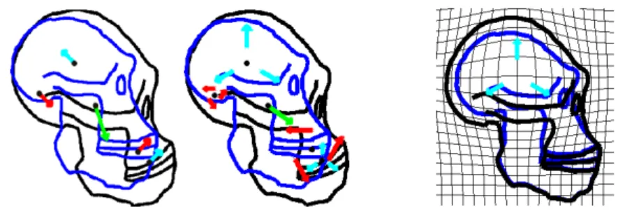
Fig. 5. Initial positions for modules : in red rotations, in green translation and in cyan scaling. In blue is the initial shape, in black the shape at t = 1. Left: parametrization of the vector field : initial geometrical descriptors (in black) and momenta. Right: Initial ge-ometrical descriptors, controls and intermediate tools.
Fig. 6. In blue the initial shape, in cyan are interme-diate tools useful to build the vector field at t = 0, in black is the transported shape while following the largest scaling.
where A(o) is a matrix depending on o. The whole geodesic trajectory is then parametrized by initial values of (o, η) (of dimension twice the dimension of o). We have obtained a geodesic shooting from an element (a, η0), with η0∈ (TaO)∗, to a geodesic path (o, h) and then to a trajectory φv with v = ζ
o(h).
Remark 2. In practice we do not minimize E with fixed a end-point but mini-mize J (ot=0, h) = E(o, h)+g(ot=1) (with o such that ˙o = ξo(ζo(h))). Trajectories minimizing J are normal geodesics following equations 2 (see [2]).
5
Examples
5.1 Shooting with constrained types of local affine transformations We present here an example of geodesic trajectory created by the combination of different modules (in dimension 2): one translation (scale 100), two rotations (scales 20 and 60), two scaling (scales 50 and 20). Initial values of the geometrical descriptor (5 points : dimension 10) and the momentum (same dimension as o) define the total trajectory: it is parametrized in dimension 20. These parameters are displayed in Figure 5 as well as initial controls (lengths of directions dj for scaling and rotation), intermediate tools (zj, dj) and the transported shape. We can follow the action of a particular module Ml by fixing the trajectory of its controls hl, and integrating the new trajectory (˜v, ˜ol) such that: ˜ol(t = 0) = ol(t = 0) and for each t : ˜v(t) = ζl
˜
ol(t)(h(t)), ˙˜o
l(t) = ξl ˜
ol(t)(˜v(t)).
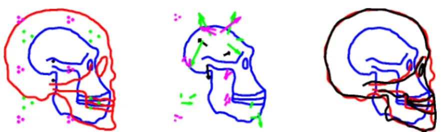
5.2 Matching with unconstrained local affine transformations We present here the matching from a shape f0to another f1, using a compound module of unconstrained local affine transformations. We set σ1 = 60, σ2= 20,
Fig. 7. Matching from f0 (blue) to f1(red), with parameters per scale (σ1: black, σ2
:green, σ3: magenta). Left: initialization geometrical descriptors. Middle: Optimized
initial geometrical descriptors and controls. Right : Match at t = 1 (black).
σ3= 8 three scales and P1= 1, P2= 9, P3= 20 the number of groups of local translations at each scale. We define O, H, V , ζ, ξ and c as in section 3.1. To each (a, η) ∈ T O∗, can be associated a geodesic trajectory of controls ha,ηand then a diffeomorphism φa,η as defined in 4. The matching problem corresponds then to finding values of a and η minimizing E(a, η, f0, f1) = ca(ha,η0 ) + λD(φa,η1 · f0, f1) where D is the varifold distance [5]. Our first implementation is adapted from the software Deformetrica where we introduce constraints to remain control points pooled during optimization. An example of result is shown on Figure 7.
6
Conclusion
We constructed a mathematical framework for generic deformation modules, which is stable under combination. Large deformations can be built then by in-tegrating vector fields generated by these modules. By defining a cost on module we allow optimal deformations to come from geodesic paths in a sub-Riemannian manifold. We presented several examples of modules and geodesics. The con-struction allows an easy interpretation of the computed deformation and the incorporation of anatomical prior, so that this work may have important appli-cations for the analysis of biological shapes.
References
1. A. Agrachev, U. Boscain, G. Charlot, R. Ghezzi, and M. Sigalotti. Two-dimensional almost-riemannian structures with tangency points. In Decision and Control, 2009 held jointly with the 2009 28th Chinese Control Conference. CDC/CCC 2009. Pro-ceedings of the 48th IEEE Conference on, pages 4340–4345. IEEE, 2009.
2. S. Arguillere. Géométrie sous-riemannienne en dimension infinie et applications à l’analyse mathématique des formes. PhD thesis, Paris 6, 2014.
3. V. Arsigny, O. Commowick, N. Ayache, and X. Pennec. A fast and log-euclidean polyaffine framework for locally linear registration. Journal of Mathematical Imag-ing and Vision, 33(2):222–238, 2009.
4. J. Ashburner. A fast diffeomorphic image registration algorithm. Neuroimage, 38(1):95–113, 2007.
5. N. Charon and A. Trouvé. The varifold representation of non-oriented shapes for diffeomorphic registration. arXiv preprint arXiv:1304.6108, 2013.
6. S. Durrleman, M. Prastawa, G. Gerig, and S. Joshi. Optimal data-driven sparse parameterization of diffeomorphisms for population analysis. In Information Pro-cessing in Medical Imaging, pages 123–134. Springer, 2011.
7. U. Grenander. Elements of pattern theory. JHU Press, 1996.
8. H. Jacobs. Symmetries in lddmm with higher order momentum distributions. arXiv preprint arXiv:1306.3309, 2013.
9. S. Joshi, P. Lorenzen, G. Gerig, and E. Bullitt. Structural and radiometric asym-metry in brain images. Medical Image Analysis, 7(2):155–170, 2003.
10. M. I. Miller, A. Trouvé, and L. Younes. On the metrics and euler-lagrange equations of computational anatomy. Annual review of biomedical engineering, 4(1):375–405, 2002.
11. M. I. Miller, L. Younes, and A. Trouvé. Diffeomorphometry and geodesic position-ing systems for human anatomy. Technology, 2(01):36–43, 2014.
12. L. Risser, F. Vialard, R. Wolz, M. Murgasova, D. D. Holm, and D. Rueckert. Simultaneous multi-scale registration using large deformation diffeomorphic metric mapping. Medical Imaging, IEEE Transactions on, 30(10):1746–1759, 2011. 13. D. Rueckert, P. Aljabar, R. A. Heckemann, J. V. Hajnal, and A. Hammers.
Diffeo-morphic registration using b-splines. In Medical Image Computing and Computer-Assisted Intervention–MICCAI 2006, pages 702–709. Springer, 2006.
14. C. Seiler, X. Pennec, and M. Reyes. Capturing the multiscale anatomical shape variability with polyaffine transformation trees. Medical image analysis, 16(7):1371–1384, 2012.
15. S. Sommer, F. Lauze, M. Nielsen, and X. Pennec. Sparse multi-scale diffeomorphic registration: the kernel bundle framework. Journal of mathematical imaging and vision, 46(3):292–308, 2013.
16. S. Sommer, M. Nielsen, S. Darkner, and X. Pennec. Higher-order momentum distributions and locally affine lddmm registration. SIAM Journal on Imaging Sciences, 6(1):341–367, 2013.
17. M. Vaillant, M. I. Miller, L. Younes, and A. Trouvé. Statistics on diffeomorphisms via tangent space representations. NeuroImage, 23:S161–S169, 2004.
18. T. Vercauteren, X. Pennec, A. Perchant, and N. Ayache. Symmetric Log-Domain Diffeomorphic Registration: A Demons-based Approach. In D. Metaxas, L. Axel, G. Fichtinger, and G. Székely, editors, Medical Image Computing and Computer Assisted Intervention, volume 5241, pages 754–761, New York, United States, Sept. 2008. Springer. pmid 18979814.
19. L. Younes. Constrained diffeomorphic shape evolution. Foundations of Computa-tional Mathematics, 12(3):295–325, 2012.
20. W. Zhang, J. A. Noble, and J. M. Brady. Adaptive non-rigid registration of real time 3d ultrasound to cardiovascular mr images. In Information Processing in Medical Imaging, pages 50–61. Springer, 2007.