HAL Id: hal-00503000
https://hal.archives-ouvertes.fr/hal-00503000
Preprint submitted on 16 Jul 2010
HAL is a multi-disciplinary open access
archive for the deposit and dissemination of
sci-entific research documents, whether they are
pub-lished or not. The documents may come from
teaching and research institutions in France or
abroad, or from public or private research centers.
L’archive ouverte pluridisciplinaire HAL, est
destinée au dépôt et à la diffusion de documents
scientifiques de niveau recherche, publiés ou non,
émanant des établissements d’enseignement et de
recherche français ou étrangers, des laboratoires
publics ou privés.
Automatic Test Generation for Data-Flow Reactive
Systems Modeled by Variable Driven Timed Automata
Omer Landry Nguena Timo, Hervé Marchand, Antoine Rollet
To cite this version:
Omer Landry Nguena Timo, Hervé Marchand, Antoine Rollet. Automatic Test Generation for
Data-Flow Reactive Systems Modeled by Variable Driven Timed Automata. 2010. �hal-00503000�
Automatic Test Generation for Data-Flow
Reactive Systems Modeled by Variable Driven
Timed Automata
Omer Nguena Timo1, Herv´e Marchand2, and Antoine Rollet1
1
LaBRI (University of Bordeaux - CNRS) Talence, France,
{nguena, rollet}@labri.fr, 2
INRIA, Centre Rennes-Bretagne Atlantique [email protected],
Abstract. In this paper, we handle the problem of conformance testing for data-flow critical systems with time constraints. We present a formal model (Variable Driven Timed Automata) adapted for such systems in-spired from timed automata using variables as inputs and outputs, and clocks. In this model we consider urgency and the possibility to fire sev-eral transitions instantaneously. We present a conformance relation for this model and we propose a test generation method using a test purpose approach. This method is illustrated with an example on a ”Bi-manual command”.
1
Introduction
Testing is one of the most popular techniques used to increase the quality of a software. Since systems are getting more and more complex, formal approaches permit to obtain efficient and rigorous testing frameworks. Testing is a large domain since many characteristics may be focused, such as conformance, per-formance, interoperability or robustness... In this paper we consider formal con-formance testing, i.e. checking if the observable behaviour of an implementation conforms to its specification described in a formal model.
Testing techniques may be very different depending on the kind of systems we intend to validate (e.g. embedded systems, communication protocols, etc...). In this work, we handle testing for critical data-flow reactive systems with time constraints. Such systems are widely used in the industrial automation domain. Data-flow reactive systems are characterized by the fact that they interact with their environment in a continuous way by means of continuous input and output set of events (taking their values in (possibly) infinite domains), while obeying some timing constraints. In this framework, continuous means that the values of the inputs events can be updated at anytime, while the value of the outputs events can always be observed. Their particularity makes that models used in testing methods (e.g. Labelled Transition Systems with inputs, outputs and/or
time) are not well adapted to describe such systems as they do not include data-flow synchronous aspects with dense time.
Related work. Timed automata [1] have been a reference model for many testing
approaches for Real-time systems. [4] and [14] propose methods based on char-acterization of states inspired from Finite State Machines (FSM) theory applied on extensions of timed automata with inputs and outputs. [6] and [14] use the region graph ([1]) as a basis for test case generation.
The LTS/ioco theory ([15]) has also inspired many testing approaches for timed systems. [11] defines new conformance relations on Timed Extended Finite State Machines (TEFSM), a timed extension of FSM. Using the LTS semantics, [7] proposes a timed extension of the ioco relation (tioco) which includes delays in the set of observable outputs. They propose two kinds of tests : one with analog-clock (dense time) and one with digital-analog-clock using a special “tick” action in the model. The Uppaal project ([9]) uses timed automata with variables and urgency to model the systems and uses a symbolic extension of ioco to generate test cases. As the previously mentioned methods, it uses an event based semantics not adapted for data-flow synchronous systems.
Many testing methods have also been proposed for data-flow synchronous systems ([3], [12], [8]). Lutess ([3], [13]) is a testing environment based on Lustre ([5]) using a “Lustre-like” model of the environment to lead test data generation. The recent version of Lutess uses Constraint Logic Programming. The Lurette environment ([12]) is similar to Lutess but uses ad-hoc notations to describe the environment. The Gatel tool ([8]) generates test cases with a white box approach : it translates the program and its environment specification into a system of constraints description and uses it to generate test data according to a test objective. All these synchronous approaches are widely used in the industry. However they do not permit to handle dense time. Timed Automata with urgent transitions, as studied in [2], allow shorter and clear specifications and it has been proved that from a language theoretic point of view, addition of urgency does not improve the expressive power of timed automata. But model in [2] is (discrete) event-based and it is not adequate for data-flow systems. To our knowledge, no approach has been proposed in the literature combining data-flow synchronous aspects and dense time.
Contributions. In this paper, we introduce the Variable Driven Timed Automata
(VDTA) model, a variant of timed automata [1] with variables, which permits to describe data-flow systems with dense time. As in [9], transitions are urgent but our model permits to fire several transitions instantaneously as long as the guard is satisfied. The inputs and the outputs of the system are variables : the tester can assign new values to the input variables and observes the output ones. In the semantics of VDTA, we consider two kinds of transitions :
– delay transitions for time elapsing
– discrete transitions including urgent transitions when the guard is satisfied,
and input-update transitions when the value of an input variable changes but the guard is still not satisfied.
From a testing point of view, we assume that the specification of the system under test is modeled by a VDTA. Our aim is then to derive a tester allowing to
check whether an implementation (that could also be modeled by an unknown VDTA) conforms with its specification. Roughly, an implementation conforms to its specification whenever after an observable sequence of input updates and delays, the values of the output variables of the implementation are the same as the ones of the specification after the same sequence.
In order to limit the number of test cases, we propose a generation method based on a selection by a test purpose allowing to target some particular behav-iors of the specification that we want to test on the implementation. We define test purposes as VDTAs equipped with a set of accepting locations playing the role of a non intrusive observer. It amounts to perform a product between the specification and the test purpose and to select the behavior leading to some particular configurations of this synchronous product (the ones that reach the accepting states of the TP). The last point is achieved by performing a core-achability analysis on a variant of the region graph derived from the VDTA and adding new constraints on the guards.
Organization of the paper. The structure of the document is as follows : Section
2 presents some definitions and notations concerning the VDTA model and its semantics. In Section 3, we introduce the notion of Time Abstract Graph and we outline the problem of reachability analysis on VDTA. Section 4 presents the conformance relation called tvco, as well as the synchronous product between two VDTAs that will be used to combine the specification and the test purpose and finally describes the symbolic test case generation methodology.
2
Model and notations
In this section, we present Variable Driven Timed Automata (VDTA), a vari-ant of timed automata extended with data, urgency and synchronous data-flow aspects : the model gives the possibility to fire several transitions (in case of successive true guards) in null delay. We also give the corresponding semantics.
2.1 Variable driven timed automata definition
Variables, Assignments, Constraints. Let N, Q+and R+denote the sets of
natural, non-negative rationals and real numbers, respectively. Let V = {V1,· · · , Vn}
be a set of variables; each variable Vi∈ V ranges over a (possibly infinite) domain
Dom(Vi) in N, Q+ or R+. We define Dom(V ) = Πi∈[1..n]Dom(Vi), the domain
of V . In the sequel, vi denotes a valuation of the variable Vi and v the tuple
of valuations of the set of variables V . A variable assignment for V is a tuple
Πi∈[1..n]({Vi} × (Dom(Vi) ∪ {⊥})) and we denote by A(V ) the set of variable
assignments for V . Given a valuation v = (v1,· · · , vn) of V and a variable
assign-ment A ∈ A(V ), we define the tuple of valuations v[A] as v[A](Vi) = c if (Vi, c) is
an element of A and c 6= ⊥, and v[A](Vi) = viotherwise. Intuitively, an element
(Vi, c) of variable assignment A, requires to assign c to the variable Vi if c is a
constant from Dom(Vi); otherwise c is equal to ⊥ and no access to the variable Vi
should be done. V ar(A) denotes the set of variables of V that are updated by A. We denote IdV the identity variable assignment that let unchanged all the
combinations of simple constraints of the form Vi⊲⊳ cwith Vi∈ V , c ∈ Dom(Vi)
and ⊲⊳∈ {<, ≤, =, ≥, >}. Given G ∈ G(V ) and a valuation v ∈ Dom(V ), we write v |= G when G(v) ≡ true. We denote P rojVi(G) ∈ G(V \ {Vi}) the
con-straint such that (v1,· · · , vi−1, vi+1,· · · , vn) |= P rojVi(G) if and only if there
exists vi ∈ Dom(Vi) such that (v1,· · · , vn) |= G. We extend in a natural way
this projection to a subset V′ of V and we denote it P roj V′(G).
Let X = {X1,· · · , Xk} be a set of clocks. A clock valuation for X is a function
from X to R+. Given X, the set of valuations is denoted RX+. Given a valuation
x= (x1,· · · , xk) ∈ RX+ and t ∈ R+, x + t stands for (x + t)(Xi) = xi+ t for any
Xi∈ X. Let X′⊆ X, x[X′ ← 0] is the valuation defined by x[X′← 0](Xi) = 0
for any Xi∈ X′ and x[X′ ← 0](Xi) = xi otherwise. We denote by G(X) the set
of clock constraints defined as boolean combinations of simple constraints of the form Xi ⊲⊳ c with Xi ∈ X, c ∈ N and ⊲⊳∈ {<, ≤, =, ≥, >}. Given GX ∈ G(X)
and x ∈ RX
+, we write x |= GX when G(x) ≡ true.
VDTA and Semantics. Variable Driven Timed Automata (VDTA) is a variant
of timed automata. The main difference with timed automata with variable is that actions are assignments of variables and constraints are defined over clocks and variables. The particularity of this model is that all transitions are urgent, meaning that they must be fired as soon as guards are satisfied.
Definition 1 (VDTA). A Variable Driven Timed Automaton (VDTA) is a
tuple A = hL, X, I, O, l0, G0, ∆
Ai, where
– L is a finite set of locations, l0∈ L is the initial location,
– X = {X1, X2, . . . , Xk} is a finite set of clocks, – I = {I1, I2, . . . , In} is a finite set of input variables, – O = {O1, O2, . . . , Om} is a finite set of output variables,
– G0∈ G(I, O) is the initial condition, a constraint with variables in I ∪ O.
– ∆A⊆ L × G(I, O, X) × A(O) × 2X× L is the transition relation:
hl, G, A, X , l′i ∈ ∆
A is a transition such that
• l and l′ are the source and the target locations of the transition.
• G is a is a boolean combination of elements of G(I), G(O) and G(X). • An output assignment A ∈ A(O).
• X ∈ 2X is a set of clocks that are reset when triggering the transition.
In the sequel, we write l−−−−→ lG,A,X ′ when hl, G, A, X , l′i ∈ ∆
Aand GA(l) = {G ∈
G(I, O, X) | ∃l′ ∈ L, l −−−−→ lG,A,X ′}. The environment of a system modeled by
a VDTA observes all the variables. The set I of input variables represents the variables to which the environment (e.g. the tester) can assign a value whereas the set O of output variables represents the variables for which the values are up-dated by the system while triggering a transition. Furthermore, we assume that all the transitions are urgent, meaning that as soon as the guard of a transition is satisfied, the transition is triggered. We also assume that the assignment of new values to the input variables is performed instantaneously. Finally, note that in each location the environment can choose any value for the input variables.
Remark 1. One can also add invariants w.r.t. the input variables in locations in
order to model some environment constraints.
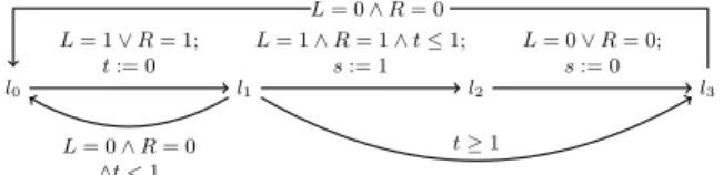
Example 1. We illustrate the previous definition with the following example de-scribing the behavior of a Bi-manual command system [10]. Consider the control program of a device designed to start some machine when two buttons (L and R for left and right buttons) are pushed within 1 time unit. If only one button is pushed (then L or R is true) and a delay of 1 time unit is performed (time-out has occurred), then the whole process must be started again. After the machine has started (s=1), it stops as soon as one button is released, and it can start again only after both buttons have been released (L and R are both false).
l0 l1 l2 l3 L= 0 ∧ R = 0 L= 1 ∨ R = 1; t:= 0 L= 0 ∧ R = 0 ∧t <1 L= 1 ∧ R = 1 ∧ t ≤ 1; s:= 1 L= 0 ∨ R = 0; s:= 0 t ≥1
Fig. 1.The ”Bi-manual command” Example
Figure 1 represents the VDTA model of this system. The model has two boolean input variables (L, R), one boolean output variable (s) and a clock (t). Let us present two important use cases of the model:
1. From the initial location l0, if L and R are both set to 1, the system must
go instantaneously to l2after starting the machine (s := 1). This is done by
taking in urgency and successively two transitions.
2. If the system reaches l1 with L = 0 and R = 1, then in order to reach
l2 or l0, it must leave l1 strictly before 1 time unit, otherwise, the system
moves instantaneously to the location l3. This is possible since transitions
are urgent.
These two use cases illustrate the utility of this new formalism : such behaviours are not natural to describe in usual event based models, even with Uppaal ([9]). Our attempts to model this system with UPPAAL 4.0 failed as invariants are bounded constraints and timing constraints are not allowed on urgent transitions which does not ease to model the urgency that can happen in l1.
Definition 2 (deterministic VDTA). A VDTA A = hL, X, I, O, l0, G0, ∆
Ai
is deterministic if
– the initial condition G0 is satisfied by at most one valuation (i0, o0), and
– for all l ∈ L, for all G, G′ ∈ G
A(l) s.t. G 6= G′, G ∩ G′ is unsatisfiable.
In the reminder of this paper, we shall only consider deterministic VDTAs.
The semantics of a VDTA is presented in terms of timed transition systems
(TTS).
Definition 3. The semantics of a VDTA A = hL, X, I, O, l0, G0, ∆
Ai, is a TTS
– S = L × Dom(I) × Dom(O) × RX
+ is the (infinite) set of states,
– s0= (l0, i0, o0, x0) is the initial configuration where x0 is the clock valuation
that maps every clock to 0 and (i0, o0) is the only solution of G0,
– Σ = A(I) ∪ A(O) ∪ RX
+ is the (infinite) set of actions, and
– → is the transition relation with the following three types of transitions:
T1 (l, i, o, x) −A→ (l′, i, o[A], x[X ← 0]) if there exists (l, G, A, X , l′) ∈ ∆ A
such that (i, o, x) |= G,
T2 (l, i, o, x)−A→ (l, i[A], o, x) with A ∈ A(I) if ∀(l, G, A′,X , l′) ∈ ∆
A, (i, o, x) 6|= G. T3 (l, i, o, x)−→ (l, i, o, x+δ) with δ > 0 if for every δδ ′< δ, for every symbolic
transition (l, G, X′, l′) ∈ ∆A, we have (i, o, x + δ′) 6|= G.
The semantics considers two kinds of transitions: discrete transitions (T1 and
T2) and delay transitions (T3). They concern the update of either input or
out-put variables. There are two sorts of discrete transitions: urgent transitions (T1) and input-update transitions (T2). Delay transitions (T3) represent the elapse of time. Urgent transitions (T1) are fired as soon as constraints are satisfied by the current configuration of the system. Input-update transitions (T2) only allow to change the values of input variables; they are fired when the environment chooses to update them and when the guards are not satisfied. Input-update transitions and delay transitions are fired only when no urgent transition can be fired. Compared with the model in [2], in our model, events (input-update) from the environment are not explicitly specified. This make VDTA specification shorter and clearer.
Notations. When necessary, we denote −→Ti for transitions of type Ti, i= 1...3.
Given a state s = (l, i, o, x) ∈ S, Out(s) = o gives access to the output value of [[A]] in state s. We write s −→ when there exists sa ′ such that s a
−→ s′. For a
sequence σ = a1.a2. . . . .ak−1.ak of Σ∗, s −→ sσ ′ if there exists {si}i=1..k−1 such
that s −→ sa1 1 −→ . . . . .a2
ak−1
−−−→ sk−1 −→ sak ′ and we write s −→ if there exists sσ ′
such that s −→ sσ ′. Given a state s of [[A]], a run is a sequence of alternating
states and actions s = s0a1s1· · · ansn in S.(Σ.S)∗ such that ∀i ≥ 0, si ai+1
−→ si+1.
Run(s, [[A]]) denotes the set of runs that can be executed in [[A]] starting in state s and we let Run([[A]]) = Run(s0,[[A]]). The trace ρ(r) of a run r = s
0a1s1· · · ansn
is given by the sequence ρ(r) = P rojS(r) = a1· · · an∈ Σ∗. T r([[A]]) = {ρ(r)|r ∈
Run([[A]])} is the set of traces generated by A.
Example 2. Back to Example 1, some possible runs derived from [[A]] are
– (l0,(0, 0, 0, 0)) L :=1 −−−→ (l0,(1, 0, 0, 0)) IdO −−→ (l1,(1, 0, 0, 0)) 0.3 −−→ (l1,(1, 0, 0, 0.3)) – (l0,(0, 0, 0, 0)) L:=1,R:=1 −−−−−−−→ (l0,(1, 1, 0, 0))−−→ (lIdO 1,(1, 1, 0, 0))−−−→ (ls:=1 2,(1, 1, 1, 0))
We now define the classic P red operator of a set of states Q: P red(Q) = {s ∈
S | ∃s′ ∈ Q, a ∈ Σ, s a
−→ s′}. Note that P red : 2S → 2S is monotonic. We also
define P re0(Q) = Q and for i ≥ 0, P redi+1(Q) = P red(P redi(Q)). We consider
the CoReach(˙) operation allowing to compute the states from which a state in
Qcan be reached: CoReach(Q) = µX.Q ∪ pre(X). Following [?], we have that
CoReach(Q) =S
Stable VDTA and Observed runs. In a VDTA, all transitions are urgent and
several transitions can be triggered in null delay. We then consider stable states that are states from which no urgent transition can be fired. Formally a state s of [[A]] is stable whenever for every A ∈ A(O), s 6−A→. A stable run is a run that
ends in a stable state. To leave this state, either the input values need to be updated or we need to let the time elapse. A VDTA A is stable if there is no loop of unstable states in [[A]].
In the context of VDTA, a test activity consists in executing on the im-plementation a sequence in (A(I) ∪ A(O) ∪ R+)∗, and in checking whether the
output values of the implementation coincide with those in the last state of the specification after the sequence being executed. It is worth noticing that on the implementation (seen as a VDTA) many variations on outputs can occur in zero time unit and these output changes can not be observed. Thus in our testing framework, we will assume that outputs are observed only when the implemen-tation is in stable states. Given a stable state s, we will thus be interested in the next stable state (recall that VDTA are deterministic) the implementation can reach from s after the execution of an input-update Ai ∈ A(I) followed by
a sequence in (A(O) ∪ R+)∗. This leads us to introduce the notion of observed
runs. Given two stable states s, s′∈ S, we write:
– s Ai
=⇒ s′ if there exists a sequence σ = σ
1· · · σn ∈ (A(O) ∪ {0})∗ such that
s Ai
−→ s” −→ sσ ′, i.e. s′ is the unique stable state that can be reached from s
after updating the input variables with Ai, only triggering urgent transitions
in zero time unit.
– s=⇒ sδ ′ if there exists a sequence σ = σ
1· · · σn ∈ ({IdO} ∪ R+)∗ such that
s−→ sσ ′and δ =P
δi∈P rojO(σ)δi, i.e. s
′is the stable state that can be reached
by letting the time elapse during δ units of time with no output update. Let us denote by Obs(A) = (S, s0, A(I) ∪ R+,=⇒) the TTS inductively
gen-erated from [[A]] starting from s0 (that is supposed to be stable) using the two previous rules. The set of observed runs of A is then given by the set
ObsRun(A) = Run(Obs(A)), whereas the set of observed traces is given by
ObsT r(A) = T r(Obs(A)). Finally, we define s Safter α = {s′ | s=⇒ sα ′}3 and
A Safter α = s0 Safter α.
3
Time-Abstract Graph and reachability analysis
The reachability analysis amounts to checking whether, from the initial state, we can reach a target state (or location). We provide a symbolic backward reachability analysis for VDTA. The algorithm iteratively computes (urgent, input-update, time-elapsing) predecessors of states using a new representation of VDTA called time abstract graph. A Time abstract graph decomposes the clock constraints into atomic clock constraints simplifying the computation of time-elapsing predecessors as transitions are urgent.
3
3.1 Time-Abstract graph construction
From a VDTA, one can build a time abstract graph whose transitions are of two sorts: urgent transitions (U1) and time-elapsing urgent transitions (U2). Time-elapsing urgent transitions correspond to atomic timing context changing and urgent transitions allow to change the contents of output variables. Time-elapsing transitions are labelled with the special action IdOthat let unchange the
value of the output variables. The construction of time-abstract graphs is based on the standard notion of region [1] introduced for the reachability analysis of timed automata. We assume the reader is familiar with the region construction of [1] for timed automata. For the sake of completeness, we recall here the main definitions and properties we will use further.
Let X = {X1, X2, . . .} be a finite set of clocks. Recall that the value of each
clock Xi ∈ X is denoted by xi. For xi ∈ R+, ⌊xi⌋ and hxii denote the integer
part and the fractional part of xi, respectively.
Definition 4 (Clock Region). We consider a constant K ∈ N. A clock
re-gion is an equivalence class of the relation ≃K over clock valuations. For two
valuations x, x′∈ RX
+, we have x ≃K x′ iff the following conditions hold:
1. ∀Xi∈ X, xi ≤ K ⇔ x′i≤ K,
2. ∀Xi∈ X, xi ≤ K ⇒ (⌊xi⌋ = ⌊x′i⌋ and hxii = 0 ⇔ hx′ii = 0),
3. ∀Xi, Xj ∈ X, xi≤ K and xj ≤ K ⇒ (hxii ≤ hxji) ⇔ hx′ii ≤ hx′ji.
We let RegK(X) be the set of clock regions for a constant K. We recall that the
size of RegK(X) is in 2O(m. log Km) where m = |X| (see [1]). When the constant
K is clear from the context, we denote by [x] the clock region that contains
x, and by [[r]] the set of clock valuations whose clock region is equal to r. We say that a region r′ is a successor of r and we write r′ ∈ Succ(r) if there are
v∈ [[r]], v′ ∈ [[r′]] and δ ∈ R
+ such that v′= v + δ. A region r′ is the immediate
successor of r, and we write r′ = I Succ(r), if r′ ∈ Succ(r) \ {r} and there is
no region r” ∈ Succ(r) \ {r, r′} such that r′∈ Succ(r”). Note that a region can
be represented by a diagonal clock constraint that involves comparisons of two clocks. If r is a region, then Gr denotes the unique clock constraint such that
r ⊆ [[Gr]]. States of time-abstract graphs are pairs of a location and a region.
Given a state (l, r), GdsA(ℓ, r) = {G | ℓ−−−−→ ℓG,A,X ′ and [[r]] ⊆ [[P rojI∪O(G)]]} is
the set of constraints whose timing part is satisfied by the region r. So, in (l, r), we only need to change values of input variables in order to satisfy a constraint of GdsA(ℓ, r).
Definition 5 (Time-abstract graph). The time-abstract graph (TAG) of a
VDTA A = hL, X, I, O, l0, G0, ∆
Ai for a constant K is the VDTA RGK(A) =
hRegK(A), X, I, O, (ℓ0, r0), G0, ∆RGi where
– RegK(A) = L × RegK(X) is the set of states of RGK(A) – The initial state is (ℓ0, r0) where r0= {¯0}
– The transition relation, ∆RG ⊆ RegK(A) × G(I, O, X) × A(O) × RegK(A)
U1 (ℓ, r)−−−−−−−−−−−−→ (ℓP rojX(G)∧Gr,A,X ′, r′) iff ∃ℓ−−−−→ ℓG,A,X ′in A s.t. [[r]] ⊆ [[P roj I∪O(G)]] and r′ = r[X ← 0] U2 (ℓ, r) G ′ ∧Gr′,IdO,IdX −−−−−−−−−−−→ (ℓ, r′) with G′ = ¬(∨ G∈GdsA(ℓ,r)P rojX(G)) and r′= I Succ(r)
In a TAG, the timing information is also encoded in the states. We move from one state to its time-successor whenever the clocks contrainst (corresponding to the region of the time-successor) is satisfied and when the input and output constraints of the outgoing urgent transitions are not satisfied. The values of input variables can change when no urgent transition can be fired.
Proposition 1. For every VDTA A, for every natural K larger than the largest
integer constant in the clock constraints of A, ObsT r(RGK(A)) = ObsT r(A).
We observe that for every natural K larger than the largest integer constant in the clock constraints of A, for every σ ∈ ObsT r(A), Out(A Saf ter σ) =
Out(RGK(A) Saf ter σ). In the sequel, we shall only consider such K.
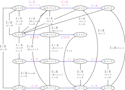
Example 3. Figure 2 represents the time-abstract graph of the VDTA in Exam-ple 1. In the figure, we have sometimes omitted to represent timing constraints on time-elapsing transitions for clarity reasons
l0, t= 0 l0,0 < t < 1 l0, t= 1 l0, t >1 l1, t= 0 l1,0 < t < 1 l1, t= 1 l2, t= 0 l2,0 < t < 1 l2, t= 1 l2, t >1 l3, t= 0 l3,0 < t < 1 l3, t= 1 l3, t >1 L ∨ R ∧t= 0 t:= 0 L ∧ R ∧t= 0 s:= 1 L ∨ R ∧ t= 0 s:= 0 L ∧ R ∧t= 0 L ∧ R ∧t= 0 L ∨ R ∧0 < t < 1 t:= 0 L ∧ R ∧0 < t < 1 L ∧ R ∧0 < t < 1 s:= 1 L ∨ R ∧0 < t < 1 s:= 0 L ∨ R ∧t= 1 t:= 0 L ∨ R ∧t >1 t:= 0 L ∧ R ∧t= 1 L ∧ R ∧0 < t < 1 L ∨ R ∧t= 1 s:= 0 L ∧ R ∧ t >1 L ∨ R ∧t >1 s:= 0 t= 1 L ∧ R ∧0 < t < 1 L ∧ R ∧t= 1 L ∧ R L xor R L xor R L ∨ R L ∧ R L ∧ R L ∧ R L ∨ R L ∨ R
Fig. 2.The TGA of the VDTA of Example 1
3.2 Backward Reachability Analysis
The simple backward control algorithm could work on [[A]]. It starts in the set of target states. Then it computes predecessors from which we can reach the target state within 1 step, 2 steps, etc... until an initial state is reached or until the computation terminates. But such a simple algorithm could not terminate
because [[A]] is infinite. We consider a symbolic algorithm that works on TAG representations instead of VDTA. We define abstract predecessors for configura-tions of TAG. A configuration of a TAG is a couple of the form (q, G) where
q is a state of RGK(A) and G is a constraint of G(I, O). We consider urgent
abstract predecessors (aP redu), time-elapsing abstract predecessor (aP redδ) and
input-update abstract predecessors (aP rede) defined over as follows:
aP redu(q, G) = {(q′, P rojX(G′) ∧ P rojV ar(a)(G) | q′ G
′
,a,Y
−−−−→U1 q
∧ P rojI∪X(G′)[a] ⊆ P rojI(G)}
aP redδ(q, G) = {(q′, P rojX(G′) ∧ G | q′ G ′ ,IdO,IdX −−−−−−−−→U2 q} aP rede(q, G) = (q, (¬WG′∈Gds A(q)P rojX(G ′)) ∧ P roj I(G))
For a set of configuration Q and θ ∈ {u, i, δ}, we define the monotonic oper-ators aP redθ(Q, G) = Sq∈QaP redθ(q, G). We define the abstract predecessor
aP red(q, G) = aP redu(q, G) ∪ aP redδ(q, G) ∪ aP rede(q, G). For a set of
con-figurations Q, aP red(Q) = S
q∈QaP red(q). Finally, CoReach(Q) = µX.Q ∪
aP re(X) We can show the following proposition that allows to use CoReacha
instead of Coreach during the reachability analysis.
Proposition 2. Given q = (l, [x]) and G ∈ G(I, O), CoReacha(q, G) = µX.(q, G)∪
aP red(X)) is effectively computable.
CoReacha is the least fixpoint of the function λX.X ∪ aP red(X) and aP red :
2Q → 2Q is a monotonic function where Q = L × Reg
K(X) × CM(I, O) and
CM(I, O) denotes the set of constraints on input/outputs the maximal constant
occuring in them is lower or equal to M . Q is finite. Using fixpoint computation results in [?], we get the termination of the computation of CoReach. Moreover, we can show that
Proposition 3. Let G′ ∈ G(I, O) be a constraints over input and output
vari-ables. It holds that
(l, i, o, x) ∈ Coreach(l′, G′∧ [x′]) iff ((l, [x]), i, o) ∈ Coreach
a((l′,[x′]), G′)
4
Automatic test generation
4.1 Principle
Conformance testing consists in checking that an implementation exhibits an observable behavior consistent with its specification. We consider conformance testing of critical timed systems modelled with VDTA. We define a conformance relation to ensure that an implementation under test (Imp) conforms to its specification. The main idea of this relation is that all behaviours of the imple-mentation have to be allowed by the specification. Especially:
1. Imp is not allowed to update a variable in a time (too late or too early) when it is not allowed by the specification.
2. Imp is not allowed to omit to change a memory-variable at the time it is required by the specification.
The conformance relation. We assume that Imp and A are both modeled by
compatible VDTA (i.e. they share the same input and output variables). More-over, we assume that the tester can observe all output variables of the implemen-tation. The tester can only update the input variables of the implementation or let the time elapse. As previously mentioned, the tester can observe the change of the output variables of the implementation only when this one has reached a stable state. As in the ioco theory [15], some states may stay infinitely blocked, but at the moment we do not consider this point in our conformance relation.
Roughly, an implementation conforms with a specification whenever it pro-duces the same outputs as the ones of the specification at the same instants.
Definition 6. Imp conforms to A (Imp tvco A) whenever
∀σ ∈ ObsTr(A), Out(Imp Safter σ) ⊆ Out(A Safter σ) where Out(.) gives access to the values of the ouput variables.
In this relation, we intend to check if the values of output variables of the imple-mentation are correct after any sequence of inputs. These inputs may be of two kinds : assignment of input variables or time elapsing. Since our model permits to fire several transitions in zero time, we decided that the implementation has to reach a stable state before checking correctness of its outputs. For example, if we consider an input followed by several assignments of the same output variable in zero time (e.g. L := 1 followed s := 3 and s := 2), our conformance relation only considers the last value (s := 2). Note that it would have been possible to define another relation, similar to tioco [7], permitting to consider all kinds of assignments for conformance. The tester who knows the specification plays in the following way:
– either the tester updates the input variables and then observes how the
implementation reacts once the implementation is stabilized. In case of non conformance (i.e. if the outputs of the implementation differ from the one of the specification), the tester returns a fail verdict;
– or the tester chooses to let the time elapse for a while; doing so, it observes
possible output changes from the implementation. In case such changes are not allowed by the specification at the time a new output observation is performed, the tester returns a fail verdict since the implementation does not conform to the specification;
– or the tester can choose to stop the game and in that case, it returns a pass
verdict meaning that, up to this point, no fault occurred.
The tester observes behaviours of the implementation through the values of the output variables in stable states. If their content changes, the tester checks whether the new values are expected by the specification.
4.2 Test purpose
The test selection algorithm we propose is based on the notion of Test Purpose (TP). In practice, a test purpose allows to select some behaviors of the specifi-cation that we want to test. A test purpose is modeled by a VDTA as follows:
Definition 7. A test purpose TP of a specification A = hL, X, I, O, l0, G0, ∆
Ai
is a deterministic VDTA hS, X ∪ X′, I, O, s0, G0, ∆
T Pi such that
– S is a finite set of locations with a special trap location AcceptT P ∈ S, s0 is
the initial location;
– I, O and X are respectively the input, output and clock variables of the
specification; TP is thus allowed to observe the configurations of A;
– G0∈ G(I, O) is the initial condition (the same as the one of A);
– X′ is the set of private clocks of T P , with X′∩ X = ∅ – ∆T P ⊆ S × G(I, O, X, X′) × IdO× 2X
′
× S is the transition relation4.
Note that T P is non intrusive with respect to the specification. Indeed, according to Definition 7, it does not reset clocks of the specification S and does not assign new values to the output variables. Moreover, we remark that all the test purposes are complete, meaning that whatever is the observation of variables or clocks either a transition is taken or the current location does not change.
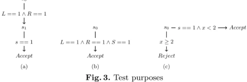
Example 4. Some test purposes for the VDTA A in Fig.1 are presented below.
s0 L== 1 ∧ R == 1 s1 s== 1 Accept (a) s0 L== 1 ∧ R == 1 ∧ S == 1 Accept (b) s0 x ≥2 s== 1 ∧ x < 2 Reject Accept (c)
Fig. 3.Test purposes
Test purposes in figures Fig.4(a) and Fig.4(b) observe variables of the VDTA and they only specify which behaviours of the implementation are interesting for the test. The test purpose in Fig.4(c) has its own clock variable x; it also specifies which behaviour of the implementation should be tested, but also the behaviour of the implementation that should not be tested (from the location Reject, the location Accept, cannot be reached anymore).
– The test purpose in Fig.4(a) requires that s will be eventually set to 1 after
the first time at which L and R are equal to 1. Between the first time in which L and R are simultaneously equal to 1 and the time in which s is set to 1, the test purpose allows, in s1, the changing of values L, R and s. The
test purpose in Fig.4(b) requires to have s equal to 1 in the same time that Land R are equal to 1.
– With the test purpose described in Fig.4(c), we are only interested in testing
behaviours of the implementation for which s is set to 1 at most 2 time units after the beginning of the session. ⋄
4
As for the specification, we assume that the guards are given by a boolean
4.3 Building the symbolic test case
Given a specification A and a test purpose T P , we now describe how to derive test cases that target the behaviour of the test purpose while checking for the conformance of the implementation with respect to the specification. It consists in three steps:
Step 1. We first perform the synchronous product between the specification
A and the test purpose in order to characterize in A the sequences that are
accepted by the test purpose T P .
Definition 8 (Synchronous product). Given A = hL, X, I, O, l0, G0, ∆
Ai a
specification and a test purpose T P = hS, X′ ∪ X, I, O, s0, G0, ∆
T Pi, the
syn-chronous product of A and T P is the VDTA A×T P = hL×S, X∪X′, I, O,(l0, s0),
G0, ∆A×T Pi where ∆A×T P is defined by the following rules (R1, R2, R3):
l−−−−→ lG,A,X ′∈ L s∈ S G s=VG′∈G T P(s)¬G ′ (l, s) G∧Gs,A,X −−−−−−−→ (l′, s) (R1) l∈ L s G,IdO,X′ −−−−−−→ s′ G l=VG′∈G A(l)¬G ′ (l, s) Gl∧G′,IdO,X′ −−−−−−−−−→ (l, s′) (R2) l−−−−→ lG,A,X ′ s G′,IdO,X′ −−−−−−−→ s′ (l, s)−−−−−−−−−→ (lG∧G′,A,X ∪X′ ′, s′) (R3)
Evolutions (transition firing) in the test purpose and the specification depend on clock values and variable values. An urgent transition can be fired in the speci-fication (and not in the test purpose) when the clocks values and the variables values satisfy no constraint on transitions from the current location in the test purpose; this situation is described by the rule R1. Conversely, an urgent
transi-tion can be fired in the test purpose (and not in the specificatransi-tion) when no urgent transition is firable in the specification; this situation is described by the rule
R2. They both trigger an urgent transition whenever the values of the variables
satisfy the guards of the specification and test purpose transitions. Recall that the test purpose and the specification are deterministic; in consequence when a transition in the specification is firable, there is at most one firable transition in the test purpose and reciprocally. This situation is described by the rule R3.
Given a specification A and a test purpose T P , we denote AT P = A × T P .
Note that A is the master of this composition in the sense that it is the only one able to change the values of the input and output variables. Due to rule R1 and
R3, there is no imposed restriction with respect to the behaviour of A. In other
words,the definition of AT P = A × T P does restrict the constraints that allow,
in A, to execute some output updates. Since input-update and delay can only be performed when the constraints that allow an output update are unsatisfiable, we can show that T r(A) = T r(AT P) and ObsT r(A) = ObsT r(AT P). In the sequel,
Remark 2. AT P has at most |L|×|S| locations andP(l,s)∈L×S((|GA(l)|×|GT P(s)|)+
2) transitions.
Step 2: Test Selection. From AT P, we build the corresponding region graph
to abstract away the time: RG(AT P) = hQ, X, I, O, q0, G0, ∆RGi. We denote
by P ass the set of locations of the form (Accept, r) ∈ Q. From the test gen-eration point of view, our aim is to generate test cases that allow to reach the
Acceptlocation. We thus consider the set of constrained configurations QP ass=
{(q, true) | q ∈ P ass} and we compute the set of coreachable corresponding
con-straints. It is given by CoReacha(QP ass) = ∪P ∈QP assCoReacha(P ). Intuitively,
during the computation of CoReacha(QP ass), if we encounter a symbolic state
(q, G) of RGK(AT P) with G as constraint on the input/output variables, then
there will exist a path giving a way to move from q to P ass by letting the time elapse or by changing inputs conveniently in encountered locations along the path. Note that when computing CoReacha(q, G) for a given symbolic state
(q, G) of RGK(AT P), we can tag visited locations q of RGK(AT P) with
ade-quate constraints on the input/output variables. We call a symbolic test case, a path from the initial location of RGK(AT P) to a P ass location.
4.4 Test case execution
We assume that we have selected a symbolic test case that is a path in RGK(AT P)
that ends in a location of the form (Accept, r) of P ass for some region r. Let T C = p0.p1. . . pn be such a symbolic test case where in each position
pk = ((lk, rk), Ik) with k = 1..n, lk denotes a location of the specification, with
ln = AcceptT P, rk denotes a region and Ik denotes a constraints (invariant)
over input/output variables computed w.r.t. CoReacha(Qpass). We provide an
on-the-fly testing algorithm for T C. The algorithm works as follows:
Let j be the position in the symbolic test case that contains the current stable state stj = ((lj, rj), ij, oj, xj) and Otrj= σ1· · · σj ∈ (A(I) ∪ R+)∗ be the
sequence played on the implementation so far.
Begin loop
(a) If (lj, rj) ∈ P ass and Out(Imp Saf ter Otrj) = oj then exit loop and
return the verdict “pass”.
(b) Choose either to delay, or to perform an input-update
The decision is to perform an input-update.
i. Select an assignment Aj such that (ij[AJ], oj, xj) satisfies the
constraint on the transition, in T C, starting from ((lj, sj), rj)
and compute stj+1= stj Safter Aj
ii. update the inputs of the implementation according to Aj
iii. If Out(Imp Saf ter Otrj.AJ) 6= oj+1 exit loop and return the
verdict “fail”; else stj becomes stj+1.
The decision is to delay
i. Pickup δ ∈ R+ such that (ij, oj, xj+ δ) satisfies the constraint
ii. If an output update occurs on Imp within δ′ ≤ δ time units then
compute stj+1= stj Safter δ′
iii. If Out(Imp Saf ter Otrj.δ′) 6= oj+1 exit loop and return the
verdict “fail”; else stj becomes stj+1.
End loop
5
Conclusion
In this work, we have been interested in the automatic test generation for data-flow systems. In order to model such systems, we have presented the Variable Driven Timed Automata model (VDTA) : a variant of timed automata with continuous variables partitioned into two sets : input variables and output ones. Input variables permit to control the system and output variables are considered as the observable outputs. Transitions are urgent and it is possible to fire several transitions in zero time in a synchronous way. We have also proposed a new conformance relation adapted to our model, and a test generation method with a selection based on a test purposes.
An interesting extension of this work would be to handle blocking states in the conformance relation. Besides, we also intend to consider assignments of variables with operations depending on other variable values (e.g. x := y + 3). Since reachability and coreachability problems become undecidable, we propose to use abstract interpretation and approximation techniques.
Acknowledgment
This work has been supported by the ANR5Testec Project. We also would like to thank Nathalie Bertrand and Thierry J´eron for their help.
References
1. R. Alur and D. Dill. A theory of timed automata. Theoretical Computer Science, 126:183–235, 1994.
2. Roberto Barbuti and Luca Tesei. Timed automata with urgent transitions. Acta
Inf., 40(5):317–347, 2004.
3. L. Du Bousquet, F. Ouabdesselam, J.-L. Richier, and N. Zuanon. Lutess: A
specification-driven testing environment for synchronous software. In International
Conference on Software Engineering, pages 267 –276, 1999.
4. Rachel Cardell-Oliver. Conformance testing of real-time systems with timed au-tomata specifications. Formal Aspects of Computing Journal, 12(5):350–371, 2000. 5. Paul Caspi, Daniel Pilaud, Nicolas Halbwachs, and John Plaice. Lustre: A declara-tive language for programming synchronous systems. In Symposium on Principles
of Programming Languages,POPL 1987: Munich, Germany, pages 178–188, 1987.
5
6. Abdeslam EnNouaary, Rachida Dssouli, and Ferhat Khendek. Timed wp-method: Testing real-time systems. IEEE Transactions on Software Engineering (TSE), 28(11):1023–1038, 2002.
7. Moez Krichen and Stavros Tripakis. Black-box conformance testing for
real-time systems. In Model Checking Software, 11th International SPIN Workshop,
Barcelona, Spain, April 1-3, 2004, volume 2989 of Lecture Notes in Computer Sci-ence, pages 109–126. Springer, 2004.
8. Bruno Marre and Agnes Arnould. Test sequences generation from lustre descrip-tions: Gatel. In ASE ’00: Proceedings of the 15th IEEE international conference
on Automated software engineering, 2000.
9. Marius Mikucionis, Kim Guldstrand Larsen, and Brian Nielsen. T-uppaal: Online model-based testing of real-time systems. In 19th IEEE International Conference
on Automated Software Engineering (ASE 2004), 20-25 September 2004, Linz, Austria, pages 396–397. IEEE Computer Society, 2004.
10. Houda Bel Mokadem, B´eatrice B´erard, Patricia Bouyer, and Fran¸cois Laroussinie. A new modality for almost everywhere properties in timed automata. In
CON-CUR 2005 - Concurrency Theory, 16th International Conference, CONCON-CUR 2005, San Francisco, CA, USA, August 23-26, 2005, volume 3653 of Lecture Notes in Computer Science, pages 110–124, 2005.
11. Manuel N´u˜nez and Ismael Rodr´ıguez. Conformance testing relations for timed
systems. In Formal Approaches to Software Testing, 5th International Workshop,
FATES 2005, Edinburgh, UK, July 11, 2005, Revised Selected Papers, volume 3997
of Lecture Notes in Computer Science, pages 103–117. Springer, 2005.
12. P. Raymond, X. Nicollin, N. Halbwatchs, and D. Waber. Automatic testing of reac-tive systems, madrid, spain. In Proceedings of the 1998 IEEE Real-Time Systems
Symposium, RTSS’98, pages 200–209. IEEE Computer Society Press, December
1998.
13. Besnik Seljimi and Ioannis Parissis. Using clp to automatically generate test se-quences for synchronous programs with numeric inputs and outputs. In ISSRE
’06: Proceedings of the 17th International Symposium on Software Reliability En-gineering, pages 105–116, Washington, DC, USA, 2006. IEEE Computer Society.
14. J. Springintveld, F.W. Vaandrager, and P. R. D’Argenio. Timed Testing Automata.
Theoretical Computer Science, 254(254):225–257, 2001.
15. J. Tretmans. Test generation with inputs, outputs, and repetitive quiescence. 17:103–120, 1996.
6
Appendix: Proof of Proposition 1
Proposition 1 is a corollary of Lemma 7 and Lemma 6
Proposition 1 Let A be a VDTA, for every K greater or equal to the maximal
constants clocks in A are compared to, we have that:
ObsT r(RGK(A)) = ObsT r(A)
Property 1 (Time Additivity in Obs(A)). Let δ′, δ” ∈ R
+. It holds that:
(l, i, o, x) δ
′
=⇒ (l′, i′, o′, x′) and (l′, i′, o′, x′) =⇒ (lδ′′ ′′, i′′, o′′, x′′) if and only if
(l, i, o, x)δ
′
+δ′′
Lemma 1. (l, i, o, x) is stable if and only if ((l, [x]), i, o, x) is stable.
Proof. (if) Part: Assume that (l, i, o, x) is stable, then by definition, for every A ∈ A(O), (l, i, o, x) 6−A→, or equivalently for all G ∈ GA(l), for every trG =
(l −−−−→ lG,A,X ′) either (1) (i, o) 6|= P roj
X(G) or (2) x 6|= P rojI∪O(G). Consider
now the location (l, [x]), urgent transitions starting from this location are of the form:
– t = ((l, [x])−−−−−−−−→G∧G[x],A,X U1 (l′,[x′])), with [x′] = [x][X ← 0]. For this
transi-tion, trGcan not be triggered in A because of (1) or (2). If (i, o) 6|= P rojX(G),
then obviously t can not be triggered. If x 6|= P rojI∪O(G), then as G[x] =
P rojI∪O(G), it is not possible to trigger t. – t = ((l, [x]) G
′
∧G[x′],IdO,∅
−−−−−−−−−−→U2 (l′,[x′])), with [x′] = I Succ([x]) and G′ =
G[x′]∧ (¬W
G∈GdsA(l,[x])P rojX(G)). As [[G[x′]∧ G[x]]] = ∅, we get that x 6|=
G[x′] and t can not be triggered.
(only if) Part: Assume that ((l, [x]), i, o, x) is stable, then for every a ∈ A(O),
it holds that ((l, [x]), i, o, x) 6−A→; or equivalently, for every trG = ((l, [x]) G,A,X
−−−−→
(l′,[x′])), either (i, o) 6|= P roj
X(G) or x 6|= P rojI∪O(G). We show that no urgent
transition (of type T1) can be fired from (l, i, o, x). By contradiction, if a transi-tion of type T1 can be fired from (l, i, o, x), then there would exist a transitransi-tion
tr = l G
′
,A′
,X′
−−−−−−→ l′ such that (i, o) |= P roj
X(G′) and x |= P rojI∪O(G′). Using
a dual argument to the proof of the if part, we get that there is a transition of type T1 from ((l, [x]), i, o, x), meaning that the latter state is not stable. This is a contradiction.
Lemma 2. Given A ∈ A(O) \ {IdO},
(l, i, o, x)−A→ (l′, i′, o′, x′) iff ((l, [x]), i, o, x)−A→ ((l′,[x′]), i′, o′, x′)
Proof. First note that if (l, i, o, x) −→ (lA ′, i′, o′, x′) then (l, i, o, x) is not stable
and, according to Lemma 1, ((l, [x]), i, o, x) is not stable.
(if) Part: Consider A ∈ A(O) \ {IdO}. Assume that (l, i, o, x) A
−→ (l′, i′, o′, x′),
then there exists tr = (l−−−−→ lG,A,X ′) such that (i, o) |= P roj
X(G), x |= P rojI∪O(G),
i′ = i, o′ = o[A] and x′ = x[X ← 0]. By definition, there exists in RGK(A) a
transition (l, [x]) G
′
,A,X
−−−−−→ (l′,[x][X ← 0]) with G′ = P roj
XG∧ G[x]. As G[x] is
the unique atomic clock constraint that contains [x], we have that x |= G[x]and
then the transition ((l, [x]), i, o, x)−A→ ((l′,[x′]), i′, o′, x′) exists.
(only if) Part: Conversely, assume that ((l, [x]), i, o, x) −A→ ((l′,[x′]), i′, o′, x′).
Then there exists in RGK(A) a transition tr = (((l, [x]), i, o, x) G,A,X
−−−−→ ((l′,[x′]), i′, o′, x′))
such that (i, o) |= P rojX(G), x |= P rojI∪O(G), i′ = i, o′ = o[A] and [x′] =
[x][X ← 0]. But tr is construted using some transition l G
′
,A,X
P rojX(G) = P rojX(G′), P rojI∪O(G) = G[x]and [[P rojI∪O(G)]] ⊆ [[P rojI∪O(G′)]].
As (i, o) |= P rojX(G), x |= P rojI∪O(G) we have that x |= P rojI∪O(G′) and
then the transition (l, i, o, x)−A→ (l′, i′, o′, x′) exists.
Remark 3. For every state q of RGK(A), it holds thatWG∈GRGK (A)(q)P rojX(G)
is a tautology.
Lemma 3. Let δ ∈ R+. Then,
((l, [x]), i, o, x)−→ ((lδ ′, r), i, o, x′) implies (l, i, o, x)−→ (l, i, o, xδ ′)
Proof. Assume that ((l, [x]), i, o, x) −→ ((l, r), i, o, xδ ′). Then, by definition x′ =
x+δ and for every transition ((l, [x])−−−−→ (lG,A,X ′, r′), for every δ′ < δ, P roj
I∪O(G) =
G[x] and either (i, o) 6|= P rojXG or x + δ′ 6|= P rojI∪OG. Assume now that
(l, i, o, x) 6−→, then there exists δδ ′ < δ and A ∈ A(0) such that (l, i, o, x) δ′
−→
(l, i, o, x+δ′) and (l, i, o, x+δ′)−A→ (l′, i, o′, x”). Thus there exists tr = l−−−−−→ lG′,A,X′ ′
such that (i, o) |= P rojX(G′), x+δ′|= P rojI∪O(G′), o′= o[A], and x” = x[X′ ←
0]. Note that by definition, x + δ′ ∈ [x]. Moreover, as tr is a transition of A,
there exists a transition (l, [x]) P rojX(G
′
)∧G[x],A,X′
−−−−−−−−−−−−−−→ (l′,[x”]) in RG
K(A). Clearly,
(i, o) |= P rojX(G′) and x + δ′|= G[x]involving that there is a urgent transition
of type T1 from ((l, [x]), i, o, x) when we delay for δ′. As urgent transition of
type T1 are taken prior to delay transition of type T3, we get ((l, [x]), i, o, x) 6−→δ
and this is a contradiction with the hypothesis.
Lemma 4. Let x and x′such that [x′] = I Succ([x]) and let δ ∈ R
+. (l, i, o, x)
δ
−→
(l, i, o, x′) if and only if ((l, [x]), i, o, x) δ.IdO
−−−→ ((l′,[x′]), i, o, x′)
Proof. (if) Part: Assume that (l, i, o, x)−→ (l, i, o, xδ ′), then x′ = x + δ and by
definition, for every l −−−−→ lG,A,X ′ and for every δ′ < δ either (i, o) 6|= P roj X(G)
or x + δ′ 6|= P roj
I∪O(G). By definition, there exists in RGK(A) a transition
(l, [x]) G
′
∧G[x′],IdO,∅
−−−−−−−−−−→ (l′,[x′]) such that [[G
[x′]]] ⊆ [[P rojI∪0(G′)]] and for every
G” ∈ GdsA(l, [x]), it holds that [[P rojI∪0(G′)]] ∩ [[P rojI∪0(G”)]] = ∅. As x 6|=
G[x′], and (i, o) |= P rojX(G′), a delay transition of amount δ can be fired from
((l, [x]), i, o, x), meaning that the transition ((l, [x]), i, o, x)−→ ((l, [x]), i, o, x + δ)δ
exists. Additionnaly, as x′ = x + δ and x′ |= G
[x′], we get the existence of the
urgent transition (of type T1) ((l, [x]), i, o, x + δ) IdO
−−→ ((l, [x′]), i, o, x′) with x′=
x+ δ. In conclusion we have shown that ((l, [x]), i, o, x)−→ ((l, [x]), i, o, xδ ′) IdO
−−→
((l, [x′]), i, o, x′).
(only if) part: if ((l, [x]), i, o, x) δ.IdO
−−−→ ((l′,[x′]), i, o, x′) then we have ((l, [x]), i, o, x) δ
− →
((l, [x]), i, o, x′) IdO
−−→ ((l, [x′]), i, o, x′) with x′= x+δ. Using lemma 3, we get that
Corollary 1. Let δ ∈ R+. Then, (l, i, o, x)−→ (lδ ′, i′, o′, x′) if and only if it exists
in [[RGK(A)]] a sequence of transitions
((l, [x]), i, o, x) δ1.IdO −−−−→ ((l′1,[x′1]), i′1, o′1, x′1) δ2.IdO −−−−→ . . . δn.IdO −−−−→ ((l′,[x′]), i′, o′, x′) with δ =Pn i=1δi.
Proof. The proof relies on Lemma 4
Lemma 5. Let A ∈ A(I). Then, (l, i, o, x)−A→ (l, i′, o, x) if and only if ((l, [x]), i, o, x) A
−→
((l′,[x]), i′, o, x)
Proof. (if) Part: Assume that (l, i, o, x) −A→ (l′, i′, o, x) with i′ = i[A] can be
triggered in [[A]], then no transition of type T1 can be triggered from (l, i, o, x). Thus, for every tG = (l
G,A,X
−−−−→ l′), it holds that (i, o) 6|= P roj
X(G) or x 6|=
P rojI∪O(G). For contradiction, assume that ((l, [x]), i, o, x) 6 A
−→. In that case,
there exists in RGK(A) an urgent transition tr = (l, [x]) G′
,A′
,X′
−−−−−−→ (l”, r) such
that (i, o) |= P rojXG′, P rojI∪O(G′) = G[x]and x |= P rojI∪O(G′). In turns, this
implies the existence of a transition l G”,A
′
,X′
−−−−−−→ l” with P rojX(G′′) = P rojXG′
and [[P rojI∪O(G′)]] ⊆ P rojI∪O(G”). It entails that there exists a transition
(l, i, o, x) A
′
−→ (l”, i, o[A′], x[X′ ← 0]) in [[A]] which discards the existence of the
input update transition (l, i, o, x)−→ (lA ′, i′, o′, x′). So the contradiction. (only if) Part: Similar to the (if) part
Lemma 6. Let (l, i, o, x) and (l′, i′, o′, x′) be two stable states, then
(l, i, o, x) AI
=⇒ (l′, i′, o′, x′) if and only if ((l, [x]), i, o, x) AI
=⇒ ((l′,[x′]), i′, o′, x′)
Proof. (if) Part: Assume that (l, i, o, x) AI
−−→ (l′, i′, o′, x′), then there exist a set
{Ak| k = 1..n} ⊆ A(O) ∪ {0} and a sequence of transitions in [[A]] such that
(l, i, o, x)−−→ (lAI
0, i0, o0, x0)−−→ . . .A1 −−→ (lAn n, in, on, xn)
W.L.O.G, assume that every Akbelongs ⊆ A(O); then there is a set of transitions
{lk−1
Gk,Ak,Xk
−−−−−−→ lk| k = 1..n} such that:
– i0= i[AI], o0= o, x0= x and for every 1 ≤ k ≤ n, ik = io – for every 0 ≤ k ≤ n − 1, (ik, ok, xk) |= Gk
– for every 1 ≤ k ≤ n, ok= ok−1[Ak] and xk = xk−1[Xk← 0] – (ln, in, on, xn) = (l′, i′, o′, x′)
Applying Lemma 5 and Lemma 2 we get the existence of the sequence of tran-sitions ((l, [x]), i, o, x) AI
−−→ (l0,[x0]), i0, o0, x0) −−→ . . .A1 −−→ (lAn n,[xn]), in, on, xn)
where (ln,[xn]), in, on, xn) = (l′,[x′]), i′, o′, x′). Moreover, according to Lemma 1,
both (l, [x]), i, o, x) and (l′,[x′]), i′, o′, x′) are stable states and finally,
(l, [x]), i, o, x) AI
=⇒ (l′,[x′]), i′, o′, x′). (only if) Part: Similar to the (if) Part.
Lemma 7. It holds that
(l, i, o, x)=⇒ (lδ ′, i′, o′, x′) if and only if ((l, [x]), i, o, x) δ
=⇒ ((l′,[x′]), i′, o′, x′).
Proof. This is a direct consequence of Lemmas 4 and 2 using a construction
similar to the one of the previous lemma.
7
Appendix: Proof of Proposition 3
We give a proof of Proposition 3 that establishes the link between CoReach and
CoReacha. The proposition show that we can use CoReachainstead of CoReach
during the reachability analysis.
Proposition 3 Let G′ ∈ G(I, O) be a constraints over input and outputs
vari-ables. It holds that
(l, i, o, x) ∈ CoReach(l′, G′∧ [x′]) iff ((l, [x]), i, o) ∈ CoReacha((l′,[x′]), G′)
Note that CoReach and CoReachaare least fixpoint of the monotonic
opera-tors P red and aP red. Then using Lemma 8, Lemma 9, Lemma 10 all presented below, we will show in Lemma 11 that aP red can be used instead of P red when computing predecessors of states. First of all let us make more precise the computation of predecessors of states of VDTA.
7.1 Predecessors
The semanctics [[A]] of a VDTA A is a Σ − LT S with three kind of transitions. Then, for each state s = (l, i, o, x) we consider three sorts of predecessors:
– the urgent predecessor P redu is defined by
P redu(l′, i′, o′, x′) = { (l, i, o, x) | ∃a ∈ A(O) s.t (l, i, o, x) A
−→T1 (l′, i′, o′, x′)} – the input-update predecessor P redeis defined by
P rede(l′, i′, o′, x′) = { (l, i, o, x) | ∃a ∈ A(I)(l, i, o, x) A
−→T2 (l′, i′, o′, x′)}
Note that by definition (l, i, o, x) ∈ P rede(l′, i′, o′, x′) iff l = l′, o = o′,∃a ∈
A(I) s.t i′= i[A] and (l, i, o, x) 6→ T1
– the time elapsing predecessor P redδ is defined by
P redδ(l′, i′, o′, x′) = { (l, i, o, x) | ∃ δ ∈ R+ s.t (l, i, o, x)−→δ T3 (l′, i′, o′, x′)}
Note that by definition (l, i, o, x) ∈ P redδ(l′, i′, o′, x′) iff l = l′, i = i′, o = o′,
and ∀0 ≤ δ′< δ, (l, i, o, x + δ′) 6→T1
Finally we define
P red(l, i, o, x) = P redu(l, i, o, x) ∪ P rede(l, i, o, x) ∪ P redδ(l, i, o, x)
For θ ∈ {u, i, δ}, and a set of state Q, we define P redθ(Q) = Ss∈QP redθ(s).
Note that P redθ : 2S → 2S is monotonic and then P red : 2S → 2S defined by
P red(Q) = S
s∈QP red(s) is also monotonic. For a constraint G ∈ G(I, O, X)
and a location l, the configuration (l, G) denotes a set of states and it is defined by (l, G) = {(l, i, o, x) | (i, o, x) |= G}.