Collaborative direct to store distribution : the consumer packaged goods network of the future

(1)

Collaborative Direct to Store Distribution:

The Consumer Packaged Goods Network of the Future

by

Nanette Thi Le

B.S. Management Science and Engineering, Stanford University, 2010 and

Melanie Ann Sheerr

M.B.A. Tuck School of Business, Dartmouth College, 2006 A.B. Economics, Harvard University, 2000

Submitted to the Engineering Systems Division in Partial Fulfillment of the Requirements for the Degree of

Master of Engineering in Logistics

at the

Massachusetts Institute of Technology

June 2011

6>

Signatures of Authors... -- --. ... ... . . . .

Master of Engineering in Logistics Program, Engin ring ystems Division May 6, 2011 C ertified by ...

Prof. Stephen C. Graves Abraham J. Siegel Professor of Management Science Thesis Supervisg A ccepted by ...

(

- Prof. Yosifl~heffi

Professor, Engineering Systems Division Professor, Civil and Environmental Engineering Department Director, Center for Transportation and Logistics Director, Engineering Systems Division

(2)

Collaborative Direct to Store Distribution:

The Consumer Packaged Goods Network of the Future

by

Nanette Thi Le

and

Melanie Ann Sheerr

Submitted to the Engineering Systems Division on May 6, 2011 in Partial Fulfillment of the

Requirements for the Degree of Master of Engineering in Logistics

ABSTRACT

Promotional events are a common occurrence in the grocery and drug industries. These events require consumer packaged goods manufacturers to deliver a large volume of product, beyond the typical demand, to the retailer in a short period of time. Two of these manufacturers, Manufacturer A and General Mills, are interested in exploring the benefits of an innovative distribution strategy: collaboratively shipping their promotional products direct to the retailer stores.

This thesis describes a modified minimum cost flow optimization model, which was developed to compare the costs of this multi-manufacturer collaborative distribution strategy with two more traditional distribution approaches in which each company would deliver product independently. The first traditional strategy entails independently delivering product to the retailer distribution center, from where the retailer would transport the product to the stores. The second traditional strategy involves each manufacturer independently delivering directly to the retailer stores. Using a retailer that participated in a trial implementation of this collaborative distribution strategy in 2010 as a case study, the model is solved to find the lowest cost distribution strategy for the region served by each retailer distribution center.

Results show that collaborative distribution is the most cost effective strategy in two thirds of the regions that were studied, and that this finding is fairly robust with respect to the input

parameters. However, cost savings to the supply chain from employing the optimal strategy are relatively small, with savings to the retailer coming at an additional expense to the

manufacturers. Therefore, this thesis concludes that the manufacturers' incentive to employ collaborative distribution depends upon a method of sharing savings with the retailer, or upon the expectation of increased revenue due to higher sales from employing this distribution strategy. Thesis Supervisor: Prof. Stephen C. Graves

(3)

List of Figures

Figure 1: Simplified Distribution Diagram of Flow I ... 23

Figure 2: Simplified Distribution Diagram of Flow 2 ... 24

Figure 3: Simplified Distribution Diagram of Flow 3 ... 26

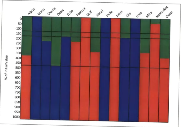
Figure 4: Cost Per Flow by Retailer DC as a Percentage of Flow 1... 39

Figure 5: Optimal Flow Selection by Retailer DC when the Comingle Fee is Varied from its In itial V alu e ... 46

Figure 6: Optimal Flow Selection by Retailer DC when the Per Stop Fee is Varied from its Initial V alu e ... 4 8 Figure 7: Optimal Flow Selection by Retailer DC when the Peddling Charge is Varied from its In itial V alu e ... 49

Figure 8: Optimal Flow Selection by Retailer DC when the Retailer Pick/Load Cost is Varied from its Initial Value... 50

Figure 9: Optimal Flow Selection by Retailer DC when the Retailer Transportation Cost is Varied from its Initial Value ... 51

Figure 10: Optimal Flow Selection by Retailer DC when the General Mills Demand is Varied from its Initial Value... 52

Figure 11: Optimal Flow Selection by Retailer DC when the MANA High Volume Category is Varied from its Initial Value... 54

List of Tables

Table 1: Modeled Trial Costs under Each of the Three Distribution Flows as a Percent of the Total Costs for Flow 1 ... 35

Table 2: Trial vs. Optimal Solution ... 35

Table 3: Representative Retailer Distribution Center Names... 36

Table 4: Optimal Flow for Each Retailer DC ... 37

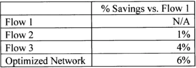
Table 5: Total Savings Relative to Flow 1 from Employing Each Distribution Strategy Across the Representative Portion of the Retailer's Network ... 40

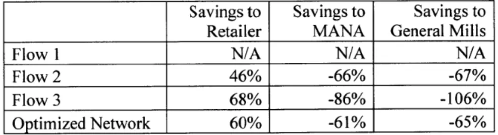
Table 6: Savings to Each Party from Employing Various Distribution Strategies... 42

Table 7: Comparison of Optimal Flow and Mixing Sites in the Base Case and All Products In stan ces... 55

(5)

I. Introduction

Large grocery and drug store retail chains procure their products from consumer packaged goods (CPG) manufacturers. Promotional events are common in this industry and drive a large volume of sales in a short period of time. For a promotional event, CPG

manufacturers provide products from multiple product families in addition to the volume that they routinely provide to the retailer. Due to the sheer volume, the manufacturers must deliver their products to the retailer in a small window of time as close to the promotion event date as possible because the retailer often cannot store that much product in advance of the promotion. This one-time, high-volume shipment presents a joint decision for the manufacturers and the retailer as to which distribution strategy they decide to employ. Each strategy has different costs,

savings, benefits, and challenges. This thesis explores an innovative multi-manufacturer

collaborative distribution strategy between Manufacturer Al (MANA) and General Mills, using a portion of one retailer's network as a case study.

The issue at hand is to investigate under what conditions co-shipping in support of promotional events can create value for the retailer and the CPG manufacturers. To this end, a

model is developed in this thesis to provide an analytical decision tool that will quantify the impacts of the distribution component of the supply chain for co-shipping directly to the retailer stores in comparison to two more typical distribution methods.

Traditionally, CPG manufacturers independently distribute product to retailer distribution centers, or in some cases, independently distribute product directly to the retailer stores.

Improper execution of promotional displays by the retailer, such as unmet promotion dates, improper assembly, incorrect display location, or, even worse, all of the above can result in

(6)

missed sales opportunity from promotions. These missed opportunities prompted MANA and General Mills to collaboratively conduct a pilot program to test a new supply network design. The two manufacturers drew on their combined scale and co-shipped products directly to a select group of stores in one retail chain in support of their joint promotion in 2010. This pilot resulted in benefits to all three parties and, as a result, warranted further exploration of this cooperative and collaborative supply chain solution. Further exploration, as has been studied in this thesis, will yield a better understanding of the conditions under which it is viable and beneficial to both manufacturers, as well as to the retailer.

The model developed in this thesis can be used as a tool that will enable a deeper understanding of transportation costs, handling costs, and other impacts of different distribution methods to support major promotional events. The model enables exploration of the costs associated with three distribution flows: independent distribution through the retailer distribution center, independent distribution directly to the retailer stores, or comingled distribution directly to the retailer stores.

First, this thesis reviews the literature on relevant distribution strategies in the industry. Second, it describes the methodology used to analyze the three distribution methods described above with a modified minimum cost flow model. Third, it covers the analysis for the pilot conducted in 2010, expands this understanding to a representative portion of the retailer's network, and investigates the sensitivity of the model's inputs. Finally, this thesis will summarize the observations garnered from the analysis.

(7)

II. Literature Review

Various methods of collaboration up and down a single supply chain have been researched, but little has been done to investigate partnerships between multiple parties who operate at the same stage in the supply chain. However, this multi-party collaboration is comparable to the case in which a single party, like a large manufacturer, uses different

collaboration strategies across its multiple supply chains, or business units. Because there are no studies on multi-manufacturer collaborative distribution, this literature review will cover

distribution strategies that have traditionally been implemented by single entities.

The distribution solution proposed by MANA and General Mills can be broken into two main components: the first is comingling goods coming from multiple locations prior to their delivery to the customer; the second is bypassing retailer distribution centers. An overview of existing distribution strategies that address each of these components is provided in the following subsections in order to provide context to the innovative multi-manufacturer collaborative

distribution strategy proposed by MANA and General Mills. Specifically, the distribution strategies discussed in this section include consolidating delivery through merge-in-transit and direct delivery through Direct Store Delivery (DSD). The benefits, drawbacks, and role of technology in each strategy are outlined in the following subsections.

II.A. Merge-in-Transit

The first distribution strategy is merge-in-transit. As Ala-Risku, Karkkainen, and Holmstrom describe, merge-in-transit is a distribution method in which separate shipments are consolidated into a single shipment for customer delivery (2003). The manufacturer stands to gain competitive advantage with this distribution strategy and could emerge as an innovative

(8)

market leader in the industry. MANA and General Mills' proposed distribution strategy is similar to using merge-in-transit in that they would combine their shipments at a consolidation point before sending it on to the retailer.

II.A. 1. Merge-in-Transit Benefits

By using merge-in-transit, the manufacturer realizes several benefits, including a gain in

competitive advantage in the market due to the increase in the customer service level from the reduced number of shipments. The fewer shipments reduce not only the handling costs incurred

by the customer, but also the administrative costs to process several orders and receipts.

Additionally, merge-in-transit can be an attractive distribution method because it reduces the inventory at the consolidation point and the need for a central distribution center. Because all of the shipments come from a different origin, such as a manufacturing plant or a distribution center, the point of consolidation requires little to no inventory on site. The manufacturer is capable of offering its customers a larger variety of products, or stock keeping units (SKUs), because it does not need to hold inventory for every single SKU at the distribution center (Ala-Risku et al. 2003). Merge-in-transit is often considered over traditional delivery to a retailer's

distribution center due to the high inventory carrying costs for the manufacturer at a central distribution center.

As Ala-Risku et al. discuss, merge-in-transit also offers the manufacturer a competitive advantage by increasing visibility throughout the supply chain. By coordinating all of the shipments, the manufacturer has better control of the material flow of its products and can better manage the cycle time between the moment the manufacturer receives the order to the moment the customer receives the delivery (2003). This visibility up and down the supply chain allows

(9)

the manufacturer to reduce its lead time in order to continue to improve its service level. It is evident that the manufacturer only stands to gain competitive advantage with merge-in-transit delivery.

II.A.2. Merge-in-Transit Challenges and Costs

While there are a number of benefits to the supply chain from using merge-in-transit, there are several challenges to the supply chain that did not exist with traditional delivery through the retailer's distribution center. Since, as Karkkainen, Ala-Risku, and Holmstrom describe, the objective is to "always fulfill one order in one delivery," delivery times on some

items may increase (2003). Sometimes it is necessary to hold off sending the first shipment until the other shipments are ready, so that the manufacturer can send all of them together in one delivery. Merge-in-transit also introduces additional costs. The main costs that a manufacturer must consider in any distribution decision, according to Karkkainen et al., are order picking costs

for the manufacturer, overhead costs for the manufacturer, transportation costs to the point of consolidation, transportation costs to the customer, and receiving costs for the customer. The new cost incurred by using merge-in-transit is the cost of consolidation (2003). Despite the

lower inventory carrying costs, there is an increase in logistics in order to consolidate the products through merge-in-transit and, thus, an increase in costs associated with organizing the

logistics. The process of coordinating multiple shipments and combining them into one delivery increases the complexity of the management necessary for the material flow (Ala-Risku et al.

2003). As a result, the greatest challenge and difficulty in implementing the merge-in-transit

(10)

function properly (Karkkainen et al. 2003). The next subsection will discuss how to alleviate this problem with the use of technology.

H.A.3. Technology Solutions

Given the large information requirements, technology is essential to the successful implementation of merge-in-transit. While a number of different software solutions are available in order to make Information Technology (IT) integration possible, there are still cases in which the information flow between different divisions of a company is not completely seamless. Regardless of the IT integration that is necessary and additional costs incurred in the

consolidation process as described in subsection above, the increase in sales alone could offset the costs and disadvantages of merge-in-transit (Karkkainen et al. 2003).

In this thesis, it is assumed that there is no technology barrier between MANA and General Mills, and that information would flow successfully between the two companies. The necessary IT integration suggested above is not in the scope of this thesis.

HA.4. Merge-in-Transit as a Viable Option

In order for the manufacturer to make merge-in-transit a viable option, it must first consider if it can satisfy several conditions. According to Ala-Risku et al., these prerequisites include the capability to serve the customer's desired order sizes, the guarantee of product availability, an acceptable delivery lead time for the customer, and the assurance of consistent lead times (2003). The manufacturer must evaluate itself to determine if it can meet these prerequisites. If these conditions can be met, then merge-in-transit can be considered as a

(11)

distribution alternative. Otherwise, it will not be worthwhile for the manufacturer to distribute its products in this way.

Mainly, the reduction of high inventory carrying costs and a more efficient transportation system will motivate the manufacturer to use merge-in-transit in order to reduce its overall costs and increase sales. The benefits realized in sales will greatly outweigh the challenges in the complexity of this distribution method. Furthermore, for large manufacturers that make

decisions based on the company's overall strategy or mission, merge-in-transit may be a good fit because it offers them the ability to provide a larger assortment of products to its customers.

There are similarities between merge-in-transit and the collaborative distribution solution proposed by MANA and General Mills. The multi-manufacturer collaborative distribution strategy also looks to consolidate shipments into a single delivery per retailer store by combining their inventory ahead of time. However, the proposed strategy differs from merge-in-transit in that it involves consolidating products from multiple manufacturers, and places the consolidation point at an existing manufacturer facility that does hold inventory.

II.A. 5. Merge-in-Transit vs. Cross-Docking

While merge-in-transit is one example of consolidating delivery, another similar alternative is cross-docking. The main difference between merge-in-transit and cross-docking lies in the goal of the strategy, according to Ala-Risku et al. (2003). Merge-in-transit focuses on sending several shipments to the customer in one delivery. The entire delivery is held off until the last shipment arrives even if the first shipment is ready to be sent. On the other hand, cross-docking aims to forward every single shipment to the final customer destination as soon as it is ready to be sent on the next available mode of transportation (Ala-Risku et al. 2003). As

(12)

pioneered by Walmart in the late 1980s, cross-docking allows customers to "receive loads containing an optimal mix and amount of products daily, while the batches arriving at the distribution centers are optimized to minimize product and process cost" (Karkkainen et al.

2003). As a result of the fast moving products to the customer, cross-docking often makes most

sense as a distribution strategy for a manufacturer with a continuous flow of goods being sent to the customer, whereas merge-in-transit would fulfill orders that are infrequent (Ala-Risku et al.

2003). Therefore, cross-docking is commonly used for distributing high volumes of commodity

products.

In the strategy proposed by MANA and General Mills as it is explored in this thesis, the cross-docking strategy is less applicable because this project focuses on one-time delivery of promotional goods, rather than high volumes of goods with constant replenishment. If MANA

and General Mills were to expand their collaboration into everyday deliveries, cross-docking might become a more viable technique for them to explore through further research.

II.B. Direct Store Delivery (DSD)

While merge-in-transit and cross-docking compare how the two manufacturers would distribute their products up to the point of consolidation, there are two ways the products can be sent to the retailer from there: either through the retailer's distribution center or directly to the retailer's stores bypassing the distribution center. The latter, a key component of MANA and General Mills' proposed distribution strategy, is referred to, in the industry, as Direct Store Delivery (DSD).

While literature discussing the topic of DSD in academia is lacking, much has been written on this topic in industry trade publications. As the Grocery Manufacturers Association

(13)

(GMA) defines it, DSD is a distribution method in which "products are delivered directly to the

store and merchandized by consumer products manufacturers" (2008). DSD began in the 1980's when the advent of computers made it possible to automate the increased volume of paperwork that DSD requires (Green & Wong 1995). The 2008 GMA study demonstrates that, almost 30 years later, DSD is viewed as an engine for driving significant sales growth.

H.B. 1. DSD Benefits to Manufacturer

Manufacturers realize two major benefits from direct store delivery: greater control over distribution and merchandizing. Manufacturers gain the ability to better control the products' environment all the way to the point of sale, which can be critical for products that are fragile, are perishable, or require a temperature controlled environment. For example, Graham discusses the case study of Edy's ice cream, which employs DSD to maintain product quality by

controlling the cold chain. Delivering products via DSD reduces the potential for a break in the cold chain by eliminating the extra step of going through the retailer distribution center, ensuring compliant carriers are used, and making sure that the ice cream is placed directly in the freezer upon arrival at the store (2001). In addition to increased control over the distribution process, there are many benefits to the manufacturer that accrue from having the products merchandized

by their own employees. Under DSD, the merchandiser has knowledge of the entire selling area,

rather than just the one chain of stores, which can provide insights leading to enhanced sales.

DSD can also allow for better shelf presentation, faster shelf set changes and incorporation of

new products, and micromarketing, such as making small corrections to the assortment to adjust for seasonality (Anonymous 1995).

(14)

IB.2. DSD Benefits to Retailer

From the retailer perspective, the main benefits result from warehousing, transportation, and labor savings. As Mathews points out, "a product 'at rest' is always an expense" and one of the largest cost to retailers is warehousing (1995). DSD enables product to bypass the retailer's warehouse completely, removing this large line item from their budget. In addition, the retailer avoids the cost of delivery from the distribution center to the stores, and associated handling costs (McEvoy 1997). Finally, as Lewis discusses, DSD creates an additional "in-store labor force" that is not paid for by the retailer (1998). This benefit may prove increasingly important

since both Karolefski and the GMA whitepaper suggest there is an "impending labor shortage. Today, it is very difficult for a retailer to find and train motivated employees for in-store

merchandizing.... With DSD providing as much as 25 percent of the retail store labor necessary for merchandizing, the retailer can focus on better serving the shopper" (GMA 2008).

H.B.3. DSD Challenges

There are many challenges associated with DSD that must be weighed against these benefits. Hjort discusses some of the difficulties with successfully implementing DSD from a manufacturer perspective. The greatest challenges are determining how often to service a retail location, and what strategy to use for each store. Typically, many stores are treated as equals for ease of management, but they should be managed independently. The cost that a manufacturer incurs to serve different stores varies widely, and so the strategy to serve each one should be developed taking into account the sales volume and rate of depletion of product (Hjort 2000).

In addition to the strategic challenges, the benefits of DSD are not always fully realized at the tactical level. As Clarke observes in a trial to reduce out-of-stocks involving Giant Eagle and

(15)

Anheuser-Busch, DSD merchandizing is not always optimal. Often the DSD deliverymen do not bring enough products, or bring the wrong assortment (2005). Shanahan, reflecting on a case study involving the Couche-Tard convenient store chain, points out that DSD can be inefficient because vendors often deliver too much product to avoid being left with partial cases (2004). Lewis raises the challenge of traffic jams at the receiving doors of retail locations, due to a separate delivery truck for each manufacturer rather than just one delivery from the retailer distribution center (1998). In addition, DSD deliverymen take more time per delivery since they spend 40% of their time merchandizing the products, which can cause long wait times for other deliverymen (ECR Report 1995). The ECR Report also states that "54 percent of all DSD deliveries are being delayed at the backdoor" (1995). Finally, DSD systems result in a significant increase in paperwork at the receiving door due to the need for documenting inventory, receiving, and invoicing (Mathews 1995).

I.B. 4. Technology Solutions

Advances in technology are frequently discussed in the literature as a method to alleviate many of the challenges with DSD. Green and Wong review the benefits of RFID technology, which allows scanners to speak directly to in-store computers to seamlessly transmit item and order information, invoicing data, and up to date discount information. Direct exchange (DEX) and network exchange (NEX) technology, which link manufacturer and retailer systems right at the backdoor, are also increasingly adopted (Green & Wong 1995, Karolefski 2008). Karolefski also discusses the trials Coca-Cola has undertaken with use of Advanced Shipment Notice

(ASN) technology which enables one bar code scan to receive an entire shipment, the detailed

(16)

reduce paperwork, shorten delivery time, and thus alleviate much of the backdoor congestion that DSD creates. Again, the scope of this thesis assumes that there are no technological barriers

in implementing DSD.

II.B.5. DSD as Delivery Strategy vs. DSD as Merchandizing Strategy

While the literature has been quite helpful in providing a deepened understanding of DSD as a merchandising strategy, it is important to note that the form of DSD discussed in all of the literature differs from what this thesis tests as a distribution option for MANA and General Mills.

MANA and General Mills have separated the merchandizing and distribution functions and plan

to implement DSD merely as a delivery method. They will deliver product directly to the stores, via their own carriers, but will leave the product at the backdoor for the store personnel to put out on display. While there is a merchandizing component to the promotion, it is not impacted by the distribution strategy selected, and is outside the scope of this thesis. Employing DSD for delivery only is noticeably absent from the literature.

Using DSD purely as a delivery option eliminates many benefits to the manufacturer that are identified in the literature. However, the savings to the retailer by way of reduced

warehousing and handling expense can still be garnered. MANA and General Mills' method of

DSD may still contribute to the traffic jam at the store receiving docks, but the comingled system

they are investigating would cut the number of trucks arriving at a given store's receiving dock in half by delivering their collective goods in the same trucks.

(17)

II.C.

Summary

The literature reviewed above has provided useful background on the benefits and drawbacks of consolidated distribution and direct delivery. In the following sections, this thesis will investigate the feasibility of a unique distribution flow which combines the two approaches - comingling goods before delivery to the customer and direct store delivery - with the added twist that multiple manufacturers are participating. The next section describes the modeling methodology employed to compare multi-manufacturer collaborative distribution to two more typical distribution methods: either the manufacturers independently distribute products through the retailer distribution center, or the manufacturers independently distribute products directly to the retailer stores.

(18)

III. Methodology

As stated in the section above, the issue at hand revolves around determining how

MANA and General Mills should distribute their products: either independent distribution

through the retailer distribution center, independent direct store delivery, or comingled direct store delivery. In the case in which both manufacturers independently distribute their products through the retailer distribution center, the retailer will send the products from that point on to its

stores. For descriptive convenience, independent distribution through the retailer distribution center will henceforth be referred to as Flow 1, independent direct store delivery as Flow 2, and comingled direct store delivery as Flow 3. The main factors in this decision are the costs associated with each of the flows. The model described in this section will aim to minimize these costs across the entire supply chain.

In this section, it is necessary, first, to understand the configuration of MANA and General Mills' current distribution networks before discussing the modeling approach taken. After the networks are explained, this section will describe linear programming in optimization problems. Then, it will outline a minimum cost network flow problem as it is the underlying

framework to this model. Next, it will expand upon this framework to describe the modified minimum cost flow optimization model that was built for this thesis to determine the least expensive routes for each of the flows as well as the least expensive flow. Finally, it will cover,

in further detail, the cost calculations used to determine the total cost of the least expensive routes for each flow. All cost terms are defined in the Glossary (Section VI).

(19)

III.A. Manufacturers' Current Networks

The two manufacturers studied in this thesis have configured their distribution networks differently. MANA ships its products directly from its manufacturing plants, and General Mills employs a network of distribution centers.

Within the scope of this project, MANA has a network of plants from which it ships directly to retailer distribution centers when employing Flow 1. Several of the plants relevant in this thesis produce a high volume product category (denoted MANA HI, H2, etc.), and the remaining sites produce low volume product categories (denoted MANA L1, L2, etc.), with each plant designated to a single category. When MANA independently employs a DSD distribution strategy, it ships all of the relevant products to one location before loading the store-bound trucks. The high volume category plant sites serve as the designated mixing locations when

MANA employs this strategy as in Flow 2. In Flow 3, the comingled DSD strategy, MANA

would ship relevant products from their respective plant locations to the mixing site, which could be any facility in the MANA or General Mills networks.

General Mills also ships products directly from its plants to retailer distribution centers, but when employing DSD or preparing special promotional pallets, they utilize their network of distribution centers. General Mills has a network of eight distribution centers across the country (denoted General Mills D1-D8) all of which carry the full complement of products. Within the

scope of this project, it is assumed that any product that General Mills delivers for a promotional event would be drawn from inventory in these distribution centers. Therefore, the distribution centers are assumed to be the General Mills product sources, and the costs associated with the transfer of goods from the manufacturing plants to the distribution centers are excluded. All

(20)

General Mills products will therefore originate from a single site, regardless of which distribution Flow is employed.

III.B. Linear Pro2rams

A linear program is an optimization problem that aims to maximize or minimize a linear

function that is constricted by linear constraints (Van Roy & Mason n.d.). The objective

function is the linear function that is being maximized or minimized. The decision variables are the terms being solved for, while the constraints specify the conditions that the decision variables must meet. Mathematically, this can be expressed in one of the following forms:

max cTx mmin cTx

subject to: Ax ! b subject to: Ax b (1)

x0 x0

The contribution (e.g. cost or profit) of each of the decision variables in the vector x is represented in the vector c. The total objective function is the dot product of the transposed vector cTwith the decision variables in the vector x. The matrix A multiplied by the decision variables list the constraints that must meet the inequality condition within the vector b. Through sophisticated computer algorithms, the values of the decision variables can be

calculated to yield the optimal solution given by the objective function while maintaining all of the conditions listed in the linear program's constraints.

III.C. Minimum Cost Network Flow Problems

A network flow problem is one of many forms that an optimization problem can take and

is applicable in many industries including agriculture, communications, defense, education, energy, health care, manufacturing, medicine, retailing, and transportation (Ahuja, Magnanti, &

(21)

Orlin 1993). In these types of problems, the decision variables represent the number of units flowing through the network from one facility, or node, to another along specified routes, or arcs. Hence, it is the basic underlying framework of the model used in this thesis because it allows

MANA and General Mills the opportunity to investigate how to distribute their products from

one node in the network to another node.

A list of all the possible routes between every pair of facilities represents all of the

possible arcs in the network. The decision variables xi1 represent the number of units that flow

along the arc from node i to node

j.

Each arc has a corresponding cost ci; and constraints: capacity ui; and non-negativity (Van Roy & Mason n.d.). This is represented mathematically as

follows:

min I cijxi;

(i,j)EA

subject to: x - xi = bi fori=1,2,...N (2)

(j:(i,j)EA} {j:(j,i)EA}

x; ; u1; V (i,j) E A

xL > 0 V (i,j) E A

In the notation in Equation (2), A is the set of arcs, where (i,j) denotes the arc from node i to node

j.

The number of nodes is given as N (Ahuja, Magnanti, & Orlin 1993). There is one flow balance constraint for each node: these constraints set the difference between the flow into the node and the flow out of the node equal to the supply at the node (bi if bi > 0) or equal to the

negative of the demand (b if bi < 0). This network is not only constrained by the capacity that

the network can handle, but also by the amount of flow required at each node. That is to say, the optimization problem aims to reduce the total cost of the network under the conditions that it does not send more units along any given arc than it can handle and that it sends at least the amount of flow that each node requires.

(22)

III.D. Modified Minimum Cost Flow Optimization Model

In the MANA and General Mills network, there are three ways that products can be distributed through the system from the manufacturer to the retailer: Flow 1, Flow 2, or Flow 3. In the model developed in this thesis, each Flow is optimized independently to determine the least expensive routes under that Flow, and then the three solutions are compared to determine the optimal Flow. The model solves for the optimal Flow for the area served by one retailer distribution center. In order to make decisions for an entire retail chain, the model is run iteratively for each distribution center.

The decision variables xi1 denote the number of pallets to send from facility i to

j.

The

cost per pallet associated with each arc is given by ciy, while the cost per truck is given by tiy. The objective is to minimize the total cost across the entire supply chain from the manufacturers to the retailer stores, subject to the constraint that the aggregate demand per product category dk is met, where k = 1, 2, ... 7. The demand at the retailer stores served by a given distribution

center (DC) is equal to the number of pallets demanded in aggregate per product category so as to ensure that the pallets flow through the network to its destination at the retailer stores. Since there are very many stores, not only is the demand aggregated per product category but the location of the retailer DC will also be used as a proxy for all the stores served by that particular

DC.

III.D. 1.Flow 1: Independent Distribution through Retailer Distribution Center

In Flow 1, the optimization model follows the basic framework of the minimum cost flow network problem discussed above with a few modifications. First, the network is laid out such

(23)

retailer DC

j

= 0. Since the total demand sent from the retailer DC to its stores, as shown in

Figure 1, is known to be equal to the total input demand, the costs associated with this segment are captured in a separate term in the objective function.

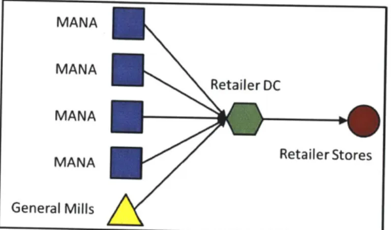
MANA MANA Retailer DC MANA Retailer Stores MANA General Mills

Figure 1: Simplified Distribution Diagram of Flow 1. Flow 1 is the case in which both

manufacturers independently distribute product to the retailer distribution center, from where the retailer would transport the product to its stores.

The cost from the retailer DC to its stores is simply included in the optimization model as additional costs per pallet

fy,

and transportation costs per pallet gps, where the selected DC is represented by the node p and the DC as a proxy for the stores by the node s. The modified optimization model for Flow 1 is as follows:

25 7

min (cioxio + Biotioxio) + (fps + gps)

Y

d,

=1k=1(3

subject to: Ixio= dk for k = 1, 2,... 7 iEHk

xio 0 V i

where xio is the number of pallets sent from facility i to the retailer DC, Bio is the number of trucks per pallet, and Hk is an index set of facilities that supply product category k. Note that in

(24)

Equation (3) there is no capacity constraint because MANA and General Mills indicated that all of their facilities relevant to the analysis in this thesis have the capacity to handle the volume associated with these types of promotions.

I.f D. 2. Flow 2: Independent Direct Store Deliverv

In Flow 2, additional constraints are necessary once MANA's policies on direct store delivery are taken into account. In DSD, MANA sends all of its products to one of its high volume plants and then distributes all products from that location directly to the retailer stores as shown in Figure 2. The MANA facilities studied in this thesis are represented as nodes i = 1, 2, ...17 and their products can be consolidated at one of the MANA high volume plants

j

= 1, 2 ... 6. Because General Mills has a network of its own distribution centers that carry its

entire product mix, it does not warrant additional constraints. The General Mills facilities

i = 18, 19, ... 25 send their products directly to the stores. Note that the retailer DC is completely

bypassed in Flow 2, as shown in Figure 2.

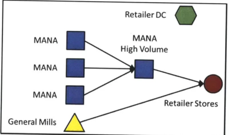
Retailer DC MANA MANA H igh Volume MANA MANA Retailer Stores General Mills

Figure 2: Simplified Distribution Diagram of Flow 2. Flow 2 is the case in which both

(25)

As in Flow 1, since the total demand that will be sent from one of the MANA designated mixing sites and the General Mills DC to the retailer stores is known, the costs associated with these segments are captured in separate terms in the objective function. The modified

optimization model for Flow 2 is as follows:

17 6 6

min _{Y (cixi + Bijtijxi;) + J[cOxjO} ₊_{(Bjotjo + gps)xjo]}

1=1 j=1

25

+ I [Cioxio + (Biotto + gps)xio]

i=18 17

subject to: x 0 forj= 1,2,...6

i=1 6 YYxi; = dk ok=12.. 4 iEHk _j=1 25

=

xIo

dk

fork = 7

i=18 x 1 0 ; Mz; for

j

= 1, 2,... 6 6 j=1 z ={0, 1} Vj XL; ;> 0 V i,j

where M is some very large number, xjO (for

j

= 1, 2, ...6) denotes the number of pallets sent

from a MANA designated mixing site to the retailer stores, and xio (for i = 18, 19, ... 25)

denotes the number of pallets sent from a General Mills facility to the retailer stores. Note that in Equation (4), there are additional binary variables zy that are necessary to select the MANA

high volume facility j = 1, 2, ... 6 where the MANA products will be consolidated. The

additional decision variables, one per MANA designated mixing site, must be binary to indicate whether or not that particular plant is the facility where all of the MANA products will be consolidated before they are sent DSD. The binary variables must sum to one so that all of the

(26)

MANA products are sent to the same designated mixing site. Finally, the last additional

constraint maintains the linearity of the binary variables.

I.f D.3.Flow 3: Comingled Direct Store Deliverv

In Flow 3, the additional constraints in Flow 2 are extended to all of the MANA and General Mills facilities because any one of them may be the consolidation point for the comingled DSD case as shown in Figure 3. As in Flow 2, Flow 3 bypasses the retailer DC.

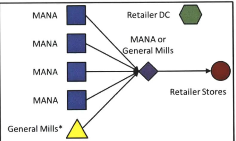
MANA Retailer DC MANA MANAor General Mills MANA Retailer Stores MANA General Mills*

* If the mixing site is a General Mills facility, then this node would not be a part of the distribution strategy. Because each General Mills distribution center contains its entire product mix, a General Mills facility would never send product to another General Mills facility.

Figure 3: Simplified Distribution Diagram of Flow 3. Flow 3 is the case in which the

manufacturers comingle their product at any one of the facilities in their combined network and distribute the product from the consolidation point directly to the retailer stores.

Again, as in Flows 1 and 2, since the total demand that will be sent from the

consolidation point, whether it is a MANA or General Mills facility i = 1, 2, ... 25, to the retailer

stores is known, the costs associated with this segment are captured in a separate term in the objective function. The modified optimization model for Flow 3 is as follows:

(27)

25 25 25

min {l cixi; + Bijtijxij) +

[c;0x;0

+ (Bjot;0 + gps)xjo]

i=1j=1 j=1

25

subject to: xi x;0 o = 0 forj = 1, 2,...25 25 xij =dk for k = 1, 2,... 7 (5) iEHk j=1 xfo s; Mz; for =1, 2,... 25 25 jz; =1 j= z; = to, 1} Vj xt; ;> 0 V i,j

Note that Equation (5) is very similar to the optimization model for Flow 2 in Equation (4) since it is an extension of the same properties to the entire network. Instead of binary variables for just the MANA designated mixing sites, there are now binary variables for all of the MANA and

General Mills facilities ] = 1, 2, ... 25. The sum of all these binary variables must be one, and

the linearity of all the binary variables is maintained.

II.D.4. Optimization Solution

Once each flow is optimized independently, each solution yields the routes that the pallets xij should be sent along from facility i to

j

in order to end up at the final destination of the retailer stores. MANA and General Mills management can determine the optimal

distribution flow in one of two ways. The flow can be chosen either because it is the least expensive or because it yields the greatest net benefit to the entire supply chain. The net benefit is determined with the expected savings relative to Flow 1 as the base and the expected sales lift that DSD yields from enhanced retailer compliance. Note that, in some cases, the least

(28)

III.E. Cost Calculations in Modified Optimization Model

The modified minimum cost flow optimization model above discusses the nature of the network and the movement of physical products. It does not explain in detail how the cost calculations affect which arcs the optimization model will select. This is contained only in the objective function, which has multiple components. The first two components are the pallet costs and transit costs for the segments in the network from the manufacturer's facilities to the point where all the products are combined before being sent to the retailer stores. In Flow 1, this point is the retailer distribution center, whereas in Flows 2 and 3, it is one of the manufacturer

facilities. The last segment, from the consolidation point to the retailer stores, is captured in two additional components, one for the pallet costs and the other for the transit costs, aggregated across the total amount of pallets being distributed to the stores. Again, all cost terms discussed in the following subsections are defined in the Glossary (Section VI).

III.E.1. Flow 1 Cost Calculations

In Flow 1, only the arcs from the manufacturers i = 1, 2, ... 25 to the retailer DC j = 0

need to be considered. The pallet costs and the transit costs of the last segment, as shown in Figure 1, from the selected retailer distribution center, represented by the node p, to its stores, represented by the node s, are captured in a separate term. The total cost for Flow 1 can be calculated as follows:

25 7

Total CoStFlow 1 = (Cioxi + Biotioxio) + (fps + g Y, dk (6)

(29)

Pallet Cost from MANA and General Mills to Retailer DCFlow 1

25

cioxio

25 ₍₇₎

= ([(MANA and General Mills Pick + Load + Unload

i=1

+ Putaway Cost) + (Damage Percentage)

* (Average Per Pallet Value)io]xio)

Transit Cost from MANA and General Mills to Retailer DCFiO1

25 25 (Floor Positions)o (8)

= Biotioxio = _{(Floor Positions Per Truck) tox1o}

7 Pallet Cost from Retailer DC to Retailer StoreSFlow 1 fps I

k=1 ₍₉₎

=(Retailer Pick + Load + Handling Cost) d k=1

7 Transit Cost from Retailer DC to Retailer StoresFiO11 = gp, dk

7k=1 (10)

=(Retailer Transportation Cost Per Pallet)I dk k=1

The damage factor in Equation (7) is only incurred when the retailer handles the products before distribution to its stores. In Flows 2 and 3, this cost is avoided in DSD through bypassing the retailer DC.

I.f E.2. Flow 2 Cost Calculations

In Flow 2, as mentioned above, MANA would send all of its products to one of the designated mixing sites and then distribute its products from that location directly to the retailer store as shown in Figure 2. In this case, the pallet costs and transit costs for MANA are split into two parts. The first part will include the arcs from the other MANA plants to the designated

(30)

mixing site at one of its high volume plants. The second part will distribute all of the MANA products from the selected high volume plant to the retailer stores. General Mills would

distribute its product from its distribution centers directly to the retailer stores as shown in Figure 2, so its costs will not be broken into separate parts. For both manufacturers, there are additional costs associated with DSD that are not applicable in Flow 1. The total cost for Flow 2 can be calculated as follows:

Total COStFIw 2

17 6 6

Z

(cijxi; + Bijtijxi;) + Z[cox;o + (Bjotjo + gps)xjo]

=1=1 j=1

25

+

j

[Cioxio + (Biot1o + gps)xio]

i=18

Pallet Cost from MANA Low Vol Plant to High Vol PlantFow 2

17 6

Y-

I

ciixi;

17 6

Y

[(MANA Pick + Load + Unload

i=1

j=1

+ Putaway Cost)xi;]

Transit Cost from MANA Low Vol Plant to High Vol PlantFlow 2

17 6

= ,Y Bijtijxi;

i=1 j=1

17 6

1

[

_{(Floor Positions)i;}

i 1(Floor Positions Per Truck) t11x1;

Pallet Cost from MANA High Vol Plant to Retailer StoreSFlow 2

6

I

cj0xj0

j=1

6

I([(MANA

Pick + Load Cost)

j=1

+ Retailer Handling Cost + DSD Receiving + DSD Storage + DSD Handling]x;0)

(11)

(12)

(13)

(31)

Transit Cost from MANA High Vol Plant to Retailer StoresFow 2

6

= (BjO tjo + gps)xjo

6 (Floor Positions);o

(Floor Positions Per Truck)

j=1 1

* [tjo + (Number of MANA Stops) (Stop Fee)]

+ [(Peddling Percentage)

* (Retailer Transportation Cost Per Pallet)]) xj 0

25

Pallet Cost from General Mills to Retailer StoreSFow 2 = ci₀_{ox 0}

i=18

25

= ([(General Mills Pick + Load Cost) (16)

i=18

+ Retailer Handling Cost + DSD Receiving + DSD Storage + DSD Handling]xio) Transit Cost from General Mills to Retailer StoreSFow 2

25

- (B_{io t}₁o + gps)xio

i=18 25

25

[((Floor

Positions)o

I ((Floor Positions Per Truck) (17) [ti; + (Number of General Mills Stops) (Stop Fee)]

* (Retailer Transportation Cost Per Pallet)]) xio]

Note that the cost calculations in Equations (16) and (17) for General Mills in Flow 2 are much like those of the last segment of Flow 1 in Equations (9) and (10) in that it is just one direct arc from the General Mills distribution center to the retailer stores.

(32)

II. E3. Flow 3 Cost Calculations

In Flow 3, all of the manufacturer facilities can send their products to any of the other manufacturer facilities before distributing them to the retailer stores as shown in Figure 3. In addition to the costs associated with DSD, there is a comingle fee to send products from one manufacturer to another manufacturer, but if a manufacturer sends its products to another one of its own facilities, the comingle fee is zero. The total cost for Flow 3 can be calculated as

follows:

Total CostFlow 3

25 25 25

-

I

cijxij

+ Bijtijxij) +

Z[c;x;o

+

(Bjot;

0

+ g,,)x;o]

(18)

i=1 j=1 j=1

Pallet Cost from MANA and General Mills to Mixing SiteFlow3

25 25

SI

cixij

i=1 j=1 (19)

([MANA

and General Mills Pick + Load + Unload

(i,j)CE

+ Putaway Cost) + Comingle Fee]xij)

Transit Cost from MANA and General Mills to Mixing Sitelow 3

25 25

I ,Bijtijxi;

i

1 x=1

(20)

25 25

_{(Floor Positions)}

1

;

I. I. [(Floor Positions Per Truck) ti] xi; i=1 j=1

25 Pallet Cost from Mixing Site to Retailer StoresFIOW 3 =

I

c;0x;0

j=' 25

- [IMANA and General Mills Pick + Load Cost) (21)

j=1

+ Retailer Handling Cost + DSD Receiving + DSD Storage + DSD Handling]x;0)

(33)

Transit Cost from Mixing Site to Retailer StoreSFow 3

25

(Bjotjo

+ gps~x;0

j=1₂₅

2S~

[(

(Floor Positions);O

I (Floor Positions Per Truck) (22)

j=1 1

[tjo + (Number of Stops) (Stop Fee)]

* (Retailer Transportation Cost Per Pallet)] _x₀

Note that this is very similar to the total cost calculated for Flow 2 because it is an extension of the same properties from the MANA DSD policies to the entire network.

III.F. Summary

The methodology outlined above illustrates how the modified minimum cost flow model was developed for this thesis. The model optimizes each of the three Flows independently, and then selects the optimal Flow that is the least expensive or the greatest net benefit to serve a particular retailer distribution center and the stores in its area. The model repeats this for each distribution center in a retail chain to determine the distribution strategies for that particular retailer. The next section will cover an analysis of the model's results from various situations.

(34)

IV. Data Analysis

The model described in the previous section was developed to test prospective

promotional events in order to determine the optimal distribution strategy. This section reveals the model's output when it is tested under various situations: first, validation of the selection of Flow 3 in a prior trial is shown; second, the results of the Base Case instance in which the model was rolled out to a representative portion of a retailer's network are presented; third, the

sensitivity of these results to the values of the input parameters is examined; and finally, some limitations of the model are discussed.

IV.A. Use of Model to Validate Preliminary Trial

The preliminary modeling objective was to validate the choice made to utilize collaborative distribution in a trial situation for a subset of the area served by one retailer distribution center (henceforth referred to as DC Charlie). The model outlined in the

Methodology section (III.D) above was programmed into Microsoft Office Excel. The actual demand for each product category from the trial promotion was provided and the manufacturers estimated values for each of the other required parameters based on their experiences in this trial.

The Excel Solver Add-In was used to solve the linear programs for each of the three Flows to select the source facilities and mixing location (if needed) that yield the minimum cost routes to serve DC Charlie. Once each Flow was individually optimized, the least expensive

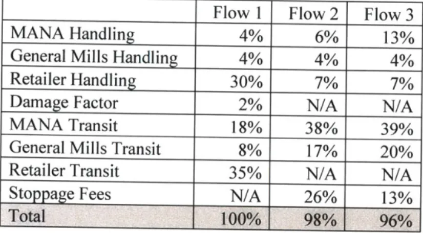
flow was chosen as the appropriate distribution strategy. The results of this preliminary model run are shown in Table 1 with all values shown as a percentage of the total Flow 1 costs. Flow 3 was found to be the least expensive distribution strategy for this DC, which validates the decision to comingle that was made in the pilot. However, the cost savings from employing this

(35)

distribution method only amount to 4% of the Flow I total distribution costs across the select group of stores in a retail chain considered in the pilot.

Table 1: Modeled Trial Costs under Each of the Three Distribution Flows as a Percent of

the Total Costs for Flow 1. Costs reflect the demand for the subset of stores served by DC Charlie that were included in the 2010 collaborative distribution trial.

Flow 1 Flow 2 Flow 3

MANA Handling 4% 6% 13%

General Mills Handling 4% 4% 4%

Retailer Handling 30% 7% 7%

Damage Factor 2% N/A N/A

MANA Transit 18% 38% 39%

General Mills Transit 8% 17% 20%

Retailer Transit 35% N/A N/A

Stoppage Fees N/A 26% 13%

Total 100% 98% 96%

While the model validates the employment of the collaborative distribution strategy, it shows that the optimal mixing site is General Mills D5, rather than General Mills D2 as was employed in the trial.

Table 2: Trial vs. Optimal Solution

Flow 3 as Implemented Flow 3 as Optimized

in Trial by Model

Mixing Site General Mills D2 General Mills D5

MANA High Volume

Source MANA HI MANA HI

MANA Low Volume

Category A Source MANA LI MANA L2

MANA Low Volume

Category B Source MANA L4 MANA L4

General Mills Source General Mills D2 General Mills D5 Total Cost as a Percent

(36)

The change in the mixing site also changes the least expensive sourcing location for some of the product categories as shown in Table 2. While the optimal site selection only contributes

1% of the Flow 1 total costs to the overall savings, this 1% represents 27% of the total benefit

from employing comingled DSD.

IV.B. Use of Model to Solve the Base Case Across Representative Portion of the Retailer Network

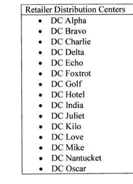
After using the model to validate the prior trial, the next phase was to expand the model across a larger portion of the retailer's chain, which included the DCs listed in Table 3. The initial instance of the model across the representative portion of this retailer's network will henceforth be referred to as the Base Case.

Table 3: Representative Retailer Distribution Center Names2

Retailer Distribution Centers

* DC Alpha * DC Bravo * DC Charlie * DC Delta * DC Echo * DC Foxtrot * DC Golf * DC Hotel * DC India * DC Juliet * DC Kilo * DC Love * DC Mike * DC Nantucket * DC Oscar

(37)

The Base Case demand estimate for each product category at each DC was proportional to the actual demand from the trial promotion. The trial demand was divided by the number of stores served in the trial to obtain a per store average demand, and this per store average was assumed to apply consistently across the retailer network.

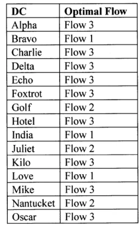
Again, using the model presented in Section III.D, the optimal flow is determined for a single DC using the Excel Solver Add-In. This process was repeated for each of the retailer DCs to create an optimal distribution strategy across the representative portion of the retailer's

network. For 60% of the retailer DCs, the optimal distribution method is Flow 3 as shown in Table 4. Of the remaining 40%, the optimal distribution method is Flow 2 for DCs Golf, Juliet, and Nantucket, and Flow 1 for DCs Bravo, India, and Love.

Table 4: Optimal Flow for Each Retailer DC

DC Optimal Flow Alpha Flow 3 Bravo Flow 1 Charlie Flow 3 Delta Flow 3 Echo Flow 3 Foxtrot Flow 3 Golf Flow 2 Hotel Flow 3 India Flow 1 Juliet Flow 2 Kilo Flow 3 Love Flow 1 Mike Flow 3 Nantucket Flow 2 Oscar Flow 3

(38)

IV B.1. Selection of Mixing Locations where Flow 3 is Optimal

In 79% of the cases where Flow 3 was selected, the mixing site chosen was the closest manufacturer facility to the retailer DC. In the remaining 21% of the cases, the optimal mixing site sources a larger product volume, even though it is slightly further away than another source facility. In the Base Case scenario solved above, the selected site was always a General Mills facility. The selection of General Mills facilities for the mixing sites is likely due to the fact that General Mills, by utilizing distribution centers of its own, has already located them close to retailer DCs in contrast to the MANA plant locations which are selected for optimal

manufacturing conditions. In addition, due to General Mills' use of a DC system, all of its products originate at the same facility, giving it a larger volume than any one of the MANA facilities. Because of this large volume, costs are minimized by moving these pallets the fewest number of times possible, so it makes sense to bring the other volume to them.

IVB.2. Cost Differences by Distribution Method

Based on the Base Case inputs provided by the manufacturers, the cost to serve each DC under all three Flows relative to the cost of Flow 1 is plotted in Figure 4. The least expensive points for each DC, shown with solid markers in the figure, taken together make up the optimized network.

Collaborative direct to store distribution : the consumer packaged goods network of the future

Collaborative Direct to Store Distribution:

The Consumer Packaged Goods Network of the Future

Master of Engineering in Logistics

Massachusetts Institute of Technology

ARCHIVES

6>

(

Collaborative Direct to Store Distribution:

The Consumer Packaged Goods Network of the Future

Table of Contents

List of Figures

List of Tables

I.

Introduction

II.

Literature Review

II.C.

III. Methodology

j.

j.

j.

j

fy,

Y

j

=

xIo

fork = 7

j

j

[c;0x;0

j

Z

j

Y-

I

ciixi;

Y

[(MANA Pick + Load + Unload

i=1

[

I

I([(MANA

[((Floor

I

cijxij

+ Bijtijxij) +

+

(Bjot;

+ g,,)x;o]

(18)

cixij

([MANA

i

(20)

(Floor Positions)

;

I

+ gps~x;0

[(

IV. Data Analysis

_{(Floor Positions)}