Climate predictability and simulation with a global climate model.

CLIMATE PREDICTABILITY AND SIMULATION WITH A GLOBAL CLIMATE MODEL

by

ALAN DAVID ROBOCK

B.A., University of Wisconsin (1970)

S.M., Massachusetts Institute of Technology (1974)

SUBMITTED IN PARTIAL FULFILLMENT OF THE REQUIREMENTS FOR THE DEGREE OF

DOCTOR OF PHILOSOPHY at the

MASSACHUSETTS INSTITUTE OF TECHNOLOGY May, 1977

Signature of Author... ... Department of Meteorology, May 1977

Certified by... Thesis Supervisor

Accepted by.;..

Committee on Graduate Students , ilil il~llm l lullil l wilill iill lt 111M -A00llllllllllllllh1

CLIMATE PREDICTABILITY AND SIMULATION WITH A GLOBAL CLIMATE MODEL

by

ALAN DAVID ROBOCK

Submitted to the Department of Meteorology.on May 5, 1977 in partial fulfillment of the requirements for the Degree of Doctor of Philosophy

ABSTRACT

Various theories of both internal and external causes of climate change on the time scale of 100 years are critically examined. Volcanic dust; solar variation; anthropogenic carbon dioxide, aerosols and heat; and stochastic variability (almost intransitivity) are all considered plausible. Data on the past variations of these forcings are collected. Observational data on climate change during the past are also assembled, and the sources of error in the data are evaluated.

A seasonal, zonally-averaged, vertically-averaged, highly-parame-terizpd numerical model, similar to that of Sellers (1973, 1974) is used to test the above theories of climate change. The model simulates the present climate fairly well, but several improvements are suggested for further studies with the model. These include more accurate formulations

of cryospheric and other seasonal variations, radiative flux, and oceanic heat flux and mixed layer depth variations.

Results show that volcanic dust and the natural atmospheric vari-ability are sufficient to explain the observed Northern Hemisphere cli-mate change of the past 100 years. Solar variation may have contributed

to the Little Ice Age, but its influence is not evident during the past 100 years. Anthropogenic carbon dioxide has a much larger effect than anthropogenic heat, and is just now becoming important enough to cause climate change. Anthropogenic aerosols are insufficiently understood to determine their effects, but may cancel out the warming effects of car-bon dioxide and heat.

Thesis Supervisor: Edward N. Lorenz

-3-ACKNOWLEDGEMENTS

I thank my thesis supervisor, Edward Lorenz, for suggesting that I study climate, for suggesting the random perturbation experiments, and for continued guidance and support throughout the writing of this thesis.

I feel privileged to have been able to work with him. I also benefited

greatly from discussions with many students and faculty in the depart-ment, whom I also thank.

I thank Stephen Schneider of NCAR for his valuable discussions of climate modeling theory, and Abraham Oort of GFDL and J. Murray Mitchell of NOAA for providing me with unpublished data.

I thank Miffi Bedrick for her love, support, and general putting up with me as I worked on this thesis, and for helping to plot some of

the figures.

I thank Isabelle Kole for her beautiful job in drafting most of the figures and Cheri Pierce for her excellent and fast typing job during a beautiful weekend when she would have rather been outside. I also thank Eve Sullivan for typing most of the rough draft.

The National Science 'Foundation supported me financially during the writing of this thesis with a Graduate Fellowship and through grant

OCD 74-03969, and the National Aeronautics and Space Administration

provided me with computer time at the Goddard Institute for Space Studies.

"The .answer, my friend, is blowin' in the wind; the answer i.s blowin' in the wind."

-5-TABLE OF CONTENTS TITLE PAGE ... ABSTRACT ... ... ACKNOWLEDGEMENTS ... ... DYLAN QUOTE ... TABLE OF CONTENTS ... . CHAPTER I. Introduction ... CHAPTER II. Climate theory ... .

A. Past climate ... 1. The data ...

2. The quality of the data ... B. Causes of climate change ...

1. External causes ...

a. Sunspots and other solar forcing ...

C.

D.

b. Volcanic dust ...

c. Anthropogenic carbon dioxide ...

d. Anthropogenic aerosols ...

e. Anthropogenic heat ...

f. Other anthropogenic effects ...

2. Internal causes (almost-intransitivity)

3. Ice age time scale causes ...

a. Intergalactic dust ...

b. Orbital variations ...

c. Continental drift ...

d. Internal causes ...

e. Ice age simulations ... Climate feedback mechanisms ...

1. The hydrological cycle ...

a. Water vapor-greenhouse ...

b. Ice (or snow)-albedo ...

c. Clouds ... 2. Ocean-atmosphere coupling ...

3. Temperature-radiation ...

4. Radiative-dynamic coupling ...

5. Temperature-lapse rate...

Different modeling aDDroaches ...

1. Model classification ...

2. Choice of a model ... a. Advantages of the model ... b. Disadvantages of the model

3. Previous simulation attempts ...

wmmw mfi I

CHAPTER III. The model ...

A. General description ...

B. The equations ...

1. Thermodynamic energy equation ...

2. Vertical profiles ...

3. Dynamical fluxes ...

a. Mean wind fluxes ...

b. Atmospheric eddy fluxes ...

c. Oceanic eddy fluxes ... 4. Surface heat storage ...

5. Solar radiation ... 6. Terrestial radiation ... C. Numerical method ... D. Differences between my model and Sellers'

1. Infrared formulation ...

2. Number of time steps ...

3. Seasonal forcing ...

4.. Smoothing ...

5. Minor differences ... E. The balanced model climate and comparison

1. The data ...

2. Temperature ... 3. Sea ice ... 4. Wind ...

5. Radiation ... 6. Horizontal heat fluxes ... 7. Summary ...

F. Parameter sensitivity ...

1. Changing parameters by 1 % ...

2. Different parameterizations ...

G. Suggestions for future model improvements

with real 0.... ... ... 0 ... .... 0.... . ... 0 .. .. . 0 ... ... ..o... 79 80 80 87 90 90 92 93 94 94 97 99 103 103 105 106 106 107 108 109 112 118 118 118 135 144 147 147 151 156 CHAPTER IV. Results ... 160

A. External causes ... 1. Design of the experiments 2. Solar forcing ... 3. Volcanic dust ... 4. Anthropogenic effects .... B. Internal causes ... 1. Design of the experiments 2. Results ... C. Geographical sensitivity... 160 160 165 167 174 178 178 180 187 CHAPTER V. Conclusions ... 190

APPENDIX A. Derivation of geopotential height equation (21) ... 193

APPENDIX B. Derivation of a coefficients, equations (24)-(34) ... 194

-7-APPENDIX C. IR model ... 200

APPENDIX D. Random number generator ... 205

REFERENCES ... 206

BIOGRAPHICAL NOTE ... 219 o1wilwo wi IN115011110111MMUME11 IN M IMIN Ifii

Chapter I. Introduction

This thesis is an attempt to better understand the causes of climate change during the period of observational record - approximately the last 100 years. Climate can be defined as a set of statistics of atmospheric variables taken over a long, but finite, time interval and a specified space domain. The time interval should be longer than a few weeks to eliminate the day-to-day changes of the weather, and it can extend all the way to ice-age time scales (104 - 106 years). The statistics can include higher moments as well as means.

The atmospheric variable that is used in this thesis to represent climate is 1000 mb or surface temperature. This is for several reasons. For more than 20 years ago, surface data is the only observational data

available. It is also the most easily deduced data from

pre-instrumental time. Temperature has an advantage over precipitation in that it has a much smoother distribution in time and space, so that fewer observations are necessary to represent its field. Furthermore, the energy balance equation makes it an easy variable to calculate. And it must be calculated in any case in order to calculate important responses of the climate system, for instance heat storage in the oceans and the ice-albedo feedback.

An understanding of climate change is important to society for several reasons. Seasonal forecasting would allow more efficient use

o'f scarce energy resources and would allow farmers to plan the proper

-9-important to be able to separate the natural fluctuations from those inadvertently caused by man, to allow us to modify our activities to prevent unwanted climate changes. Along the same line, suggestions are already being made as to how man could advertently modify the climate. Much more study and understanding of the complex nature of the system and all its feedbacks is necessary before such actions should be con-sidered.

The approach of this thesis is to use a numerical model to try to simulate the observed climate changes of the past 100 years, for-cing it according to the different plausible theories of climate change. The model is the global, seasonal, highly-parameterized, energy-balance climate model of Sellers (1973, 1974), modified and corrected for use in this thesis. It had ,een newly developed at the time this thesis was begun, and had not been applied to the problem of time-dependent climate change.

The first step was to collect and analyze the data on past cli-mate change. This is done in Chapter II. This chapter also contains a detailed analysis of the possible causes of climate change during the past 100 years, and the data describing these forcings. The next

chap-ter describes the model and the changes made in it, and compares its seasonal cycles and annual average fields of temperature, radiation and heat fluxes to the available observations. Suggestions are made as to how the model might be improved to correct the deficiencies noted in

the data comparison, but the derivation of new parameterizations is beyond the scope of this thesis. Chapter IV presents the results of

the simulation attempts with the model, and also examines internally

caused climate change, which relates to climate predictability. Chapter V is the conclusion.

The model does quite a good job of simulating the present annual averaged climate, and the seasonal cycle. Certain parameterizations need to be improved, however, before further studies are done with it. The most important and obvious ones are the seasonal cycle of ice and snow, zenith angle albedo effects, and the ocean heat flux. Once these corrections are made, the model shows great promise for further use in simulating climate change.

The model simulation experiments allow the climate change of the past 100 years to be completely explained by volcanic dust and natural variability. Solar forcing does not play a role, and anthropogenic effects are not yet of a magnitude to be observable. These statements are subject to the limitations of an imperfect model, data inadequate both in coverage and accuracy, and lack of understanding, or inclusion,

-11-Chapter II. Climate Theory

In order to understand the significance of the work done in this thesis, it is important to know what the past climate has been and what the present state of the theory of climate is. This chapter will review our present knowledge of the past climate and the quality of these ob-servations. It will discuss possible causes of climate change and

analyze the data available on the variations of these forcings over the past 100 years. It will describe climate feedback mechanisms and the different approaches to climate modeling. Finally, it will explain why

the model used in this thesis was chosen.

Several comprehensive survey articles are available on climate modeling. The best of these is the one by Schneider and Dickinson

(1974). It discusses many aspects of climate modeling, but does not give a very detailed view of past climate change. Included topics are definition of climate, climatic predictability, internal versus external causes of climate change, ingredients of a theory of climate, modeling methodology, and an extensive discussion of current modeling efforts of all types. The article includes an extensive bibliography.

Two other surveys were also published in 1974. One of these is the CARP (1974) report. It includes observed variability of the climate system, the physical basis of climate and climate modeling, the design of climate models, and the design of an observational program for cli-mate. The Gates and Mintz (1974) report covers much the same areas and includes a detailed plan for a National Climatic Research Program and a

detailed summary of our present knowledge of past climatic variations. The SMIC (1971) report presents a summary of past climate, the theory of climate and climate models, as well as indicating various ways in which man's activities may influence the climate of the future.

A. Past climate

1. The data

The earth is approximately 4.5 billion years old. During almost

90% of this time, there is no direct evidence for the climate of the

earth. During the past billion years there is evidence for three major glaciations of the earth: at least one from 800 million to 600 million years ago, called the Late Precambrian Glacial Age(s); one from 320 million to 250 million years ago, called the Permo-Carboniferous Glacial Age; and our present glacial age, which began only 10 million years

ago. Higher organized life began on the earth about 550 million years ago, and during 90% of the time since then the poles have been ice-free, so in this time frame, we are now in an anomalously cold period of our earth's history. During the Permo-Carboniferous Glacial Age the conti-nents were joined in one super-continent (Pangaea) and were yet to

drift to their present locations. This summary of the distant past is

by way of perspective, as this thesis will deal with time scales on the

order of 100 years into the past. The best source for climatic history is "A Survey of Past Climates", Appendix A, pp. 179-276 of Gates and Mintz (1974).

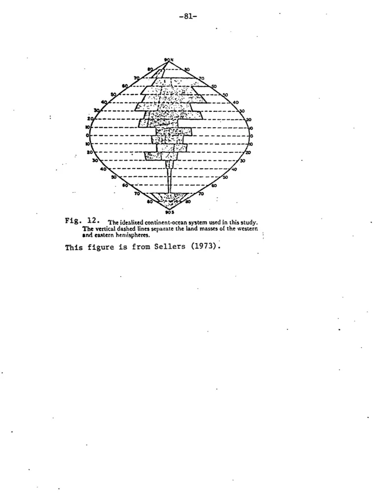
Figure 1 gives a summary of our climatic history on the longest known time scales. Continental drift played a major part in the

-13-- "" -PRESENT e% OLACIAL AG S CARBONIFEROUS GLACIAL AGE s < 251 LATE _1. PRECAM- 0 30 SRIAN 0 GLACIAL o AcEtIll -40 45 '.00 Se GUATERMARY PLIOCENE MIoCENE OLIG0-CENE EOCENE

-.- aLAST MAJOR CLIMATIC CYCLE\

...- NORTH ATLANTIC GLACIAL 3GINS

-.- ANTARCTIC ICE SMEET

ATTAINS PRE3ENT VOLUME

--- GROWTH OF N.NEMI SPNEE

MOUNTAIN GLACIER~S

EXPANSION Of ANTARCTIC ICE

I -- ANTARCTIC ICE LOCALLY

REAC"ES CONTINENTAL EDGE

ANTARCTIC CIRCUMPOLAR CURRENY SYSTEM ESTABLISNED SUDSTANTIAL COOLING OF ANTARCTIC WATERS -4 w 0

le

PRESENT INTERGLACIAL BEGINS

-- LAST GLACIAL MAXIMUM

COMPLEX Of CLIMATIC CYCLES,

MAINLY GLACIAL COMOIT ICes

SEVERE GLACIATION

COMPLEX OF CLIMATIC CYCLE

S,

MAINLY INTERGLACIAL CON OITIC;%

SEVERE POST- EEMIAM COOLIN LAST FULL IXTERGLACIAL(Eitea. PRE-EZMIAK 3LACIAL MAXIMiw

INITIAL OPENING Of

ANTARCTIC- AUSTRALIAN PASSAGE

CENOZOIC DECLINE lEG INS

Fig..

1

-- History of glacial ages over the last 1,000,000,000 years.

Intervals when extensive polar ice sheets occurred are

in-dicated as glacial ages on the left. An outline of

signif-icant events in the Cenozoic climate decline is given in

the middle, and the significant climatic events during the

last major glacial-interglacial cycle is given on the right.

This figure is from Gates and Mintz (1974).

0. 0 - 400-* 400-'.j o 400-.700' $00-I

development of the present glacial age. For the purpose of this'thesis, however, the continents will be assumed to be fixed in their present locations as part of the fixed external system. During the last

500,000 years, warm interglacials have been occurring approximately

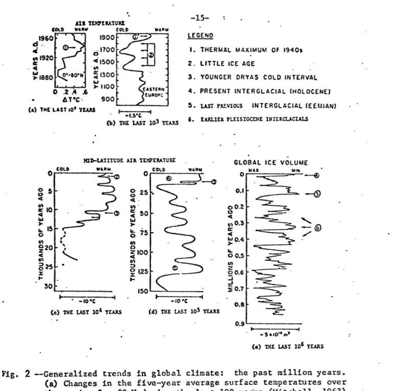
every 100,000 years. This can be seen in Figure 2e. Looked at from this perspective, we are now in an anomalously warm period between glacial maxima. The last interglacial period was approximately 125,000 years ago, and since then there have been complex variations and a gradual cooling and ice advance until 10,000 years ago when the present interglacial began. This can be seen in Figure 1 and Figure 2(d and c). The Milankovitch hypothesis has received much support recently as an explanation of climate change on this time scale. See section II.B.3 for further discussion of the causes of ice age time scale climate, changes.

The present interglacial began about 10,000 years ago, and has been basically warm with several cold intervals which did not result

in large-scale glaciation. The last cold interval occurred from 1430 to

1850 A.D. and was called the Little Ice Age. It had cold maxima about

1450 and 1650 A.D. See figures 2b and 3. The climate then warmed and continued warming until about 1940 after which there has been a cooling.

All of the previous record comes from direct evidence of

temper-ature related phenomena, in historical records when available, and before that and in addition, from evidence such as tree ring growth, oxygen isotope ratios in ice cores, tree-line and glacier margin fluc-tuations, pollen records from soil cores and fossil plankton records

All TEWERATURE

COLDO WARII COLD WARM

1960 1900 -d

_21,

₁₅₀₀

(a) THE LAST 10' YEARS

(b) THE LAST 103 YEARS

=4D-.ATITUDE AIR TEERATURE

WARM - COLD

o

~75

2. LITTLE ICE AGE

3. YOUNGER ORYAS COLD INTERVAL

4. PRESENT INTERGLACIAL (HOLOCENE)

5. LAST PRLVIOUS INTERGLACIAL (EEMIAN)

6. EARLIER PLEISTOCENE INTERCLACIALS

GLOBAL ICE VOLUME

aMIN

0 f -. - _ _

10 C _{-1-I - c .}

Cc) THE LAST 104 YEARS (d) THE LAST 105 YEARS

(e) THE LAST 106 YEARS

Fig.

2

--Generalized trends in global climate: the past million years.

(a)

Changes in the five-year average surface temperatures over

the region 0

-

80 N during the last 100 yea'rs (Mitchell, 1963).

(b) Winter severity index for eastern Europe during the last

1000 years (Lamb, 1969).

(c)

Generalized mid-latitude

North-ern

Hemisphere air-temperature trends during the last 15,000

years, based on changes in tree-lines (LaMarche, 1974),

mar-ginal fluctuations in 'a1pine and continental glaciers (Denton

and Karl6n, 1973), and shifts in vegetation patterns recorded

in pollen spectra (van der Ha-mmen

et

al., 1971).

(d)

Gener-alized Northern Hemisphere air-temperature trends during the

last 100,000 years, based on mid-latitude sea-surface

temper-ature and pollen records, and on worldwide sea-level records

(see Fig. A13).

(e) Fluctuations in global, ice-volume

dur-ing the last 1,000,000 years as recorded by changes in

iso-topic composition of fossil plankton in deep-sea core V28-238

(Shackleton and Opdyke, 1973).

See legend for identification

of symbols (1) through (6).

This figure from Gates and Mintz (1974).

WINTER

SEVERITY

200

400

600

1900

00

a

200

3

I-400

a

rig.

-- Climatic records of the past 1000 years.

(a) The 50-year moving average of a

relative index of winter severity compiled for each decade from documentary

records in the region of Paris and London (Lamb, 1969).

(b) A record of

6018

values preserved in the ice core taken from Camp Century, Greenland (Dansgaard

et

al.,

1971).

(c) Records of 20-year mean tree growth at the upper treeline

of bristlecone pines, White Mountains, California (LaMarche, 1974).

At these

sites tree growth is limited by temperature with low growth reflecting low

temperaturi.

(d) The 30-year means of :bserved and estimated annual

tempera-tuarcs over central England (Lamb, 1966).

This figure is from Gates and Mintz (1974).

-17-more and -17-more of the detailed fluctuations are lost and the evidence is more and more speculative. Only the last 100 years of this climato-logical record have been documented with instrumental observations and only in the last 25 years has there been adequate coverage of the Northern Hemisphere continents. Both the Southern ahd Northern Hemisphere oceans still lack adequate data coverage.

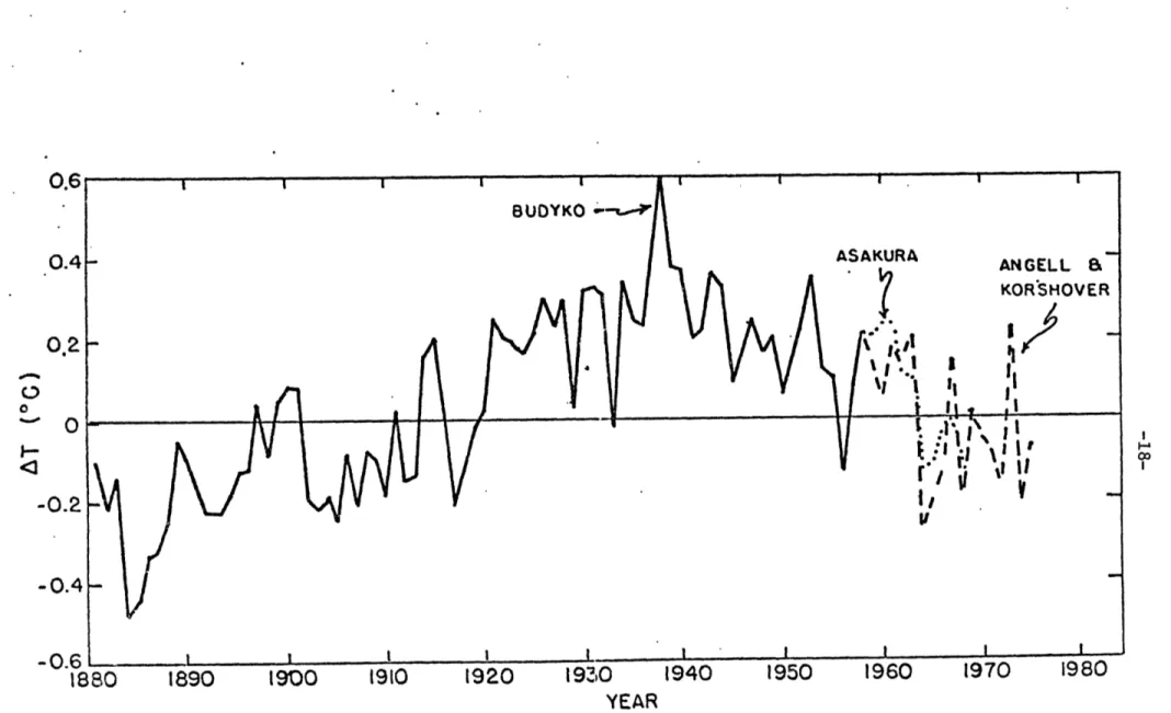
From 1880 to 1940 the annual mean Northern Hemisphere temperature rose about 1*C and since then has fallen about 0.5*C. This trend is superimposed on highly variable inter-annual changes. This can be seen in Figure 4, which shows the data of Budyko (1969), Asakura (Gates and Mintz, 1974) and Angell and Korshover (1977). The same trend can be

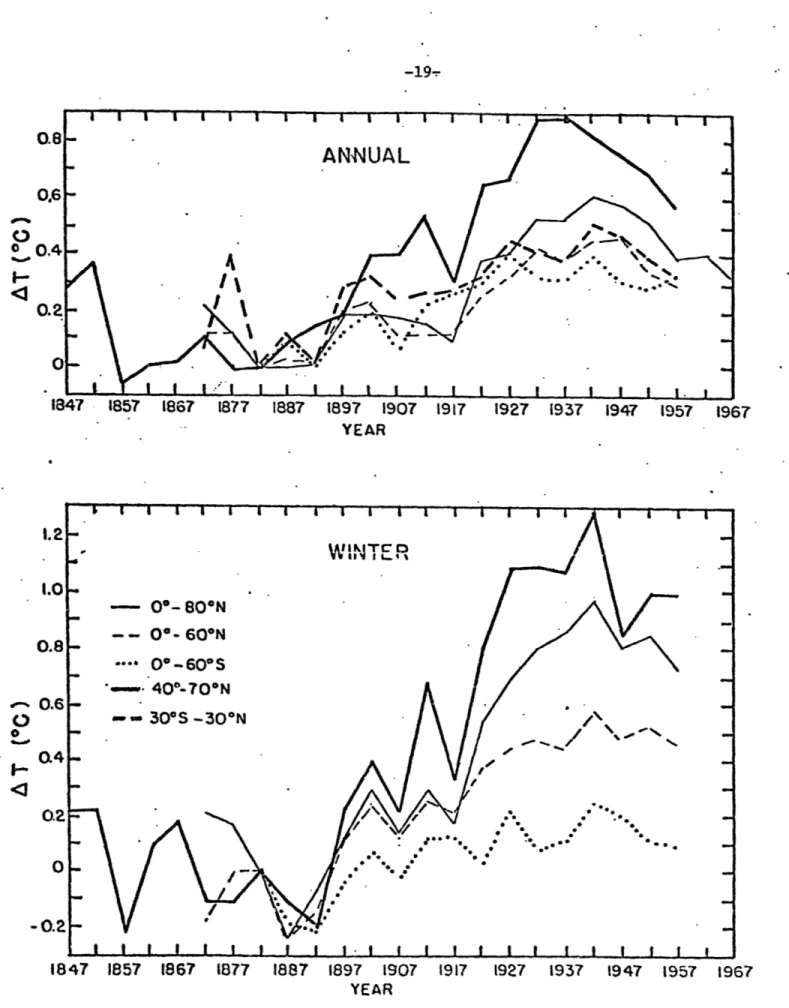
seen in the data of Mitchell (1961) (Figure 5), which is given in five-year averages, for four different latitude bands (0-80"N, 0-60*N, 0-60*S

and 40-70*N) for both annual and winter averages, and for 30*S-30*N for annual averages only. [One would not expect the tropics to exhibit winter behavior different from annual behavior.]

The above two collections of data represent the extent and qual-ity of instrumental observations of climate change on the time scale of

100 years. Several much shorter (5-30 years) data sets exist, which

include upper air and not just surface data. Starr and Oort (1973) studied the temperature change during the five-year period 1958 to 1963 from 10*S to 75*N and found an 0.6*C decrease in the mass-weighted tem-perature from the surface to 50 mb. During this same time their surface

temperature rose by 0.26*C. This change involved a considerable lapse rate change. The next 10 years of data have been collected by Oort

0.4-

A

2

-

0O--0.2

-0.4-1880

1890

1900

1910

1920

1930

1940

1950

YEAR

Figure 4. Annual mean temperature of the Northern Hemisphere for 1881-1975,

Asakura (Gates and Mintz, 1974), and Angell and Korshover (1977).

SAKURA

ANGEL L KOR'SHOV

1960

1970

1980

-19-0.4

-0.2

0

- i

i

i

L--I

I

t I

I I -I

L I .

I.

1847

1857

1867

1877

1887

1897

1907

1917

1927

1937

1947

1957

1967

YEAR

1.2

WINTER

1.0

0.8

-0-

60*N

O-60*S

--

40'-70*N

S0.6---

-- 30*S

-30*N

%--0.2

sit

YEAR

Figure 5. Five-year average temperatures by latitude bands, from Mitchell

(1961). The 0*-800N annual record is updated by Reitan (1974). The center

of the five-year averaging periods are indicat.ed on the abscissa.

collection includes the entire world-wide radiosonde network for these latitudes with sophisticated error detection and correction, so cannot be dismissed due to inaccuracy of the data. Yet on the time scale of climate change, five years is a very short time, and a longer record needs to be collected and studied before the complex changes observed during this five year period can be interpreted as typical of climate change, or as part of the random natural variability of the atmosphere.

Angell and Korshover (1975) collected sets of 300 mb and 700 mb temperatures for six different latitude bands from six fairly evenly spaced stations around each band for the time period 1958-1973. The representativeness of these few data points at only two levels remains open to question as indicative of global climate change, especially since Starr and Oort found rather unrelated changes iii the upper atmo-sphere and at the surface, yet their results are suggestive. They found quite different changes at different latitude bands and opposite changes in the two hemispheres. They also found lapse rate changes associated with mean temperature changes.

A more comprehensive collection (Angell and Korshover, 1977) will

soon be published which includes data from the surface to 100 mb for a more extensive, but still sparse, global network of 63 stations, for

1958 to 1975. They found complex changes in the vertical structure and

horizontal distribution of temperature changes. Their data for Northern Hemisphere surface temperature agree surprisingly well with those of Yamamoto, et al. (1975) who used 343 stations in the Northern Hemisphere,

an order of magnitude more. These data of Angell and Korshover, com-bined with those of Budyko in Figure 4, provide a 95 year record of the

-21-Northern Hemisphere average surface temperature, the only one with annual average values. Borzenkova, et al. (1976) have also published an analysis of Northern Hemisphere surface temperatures for 1881 to

1975, but only for latitude circles 20*N to 85*N.

Damon and Kunen (1976) studied a very sparse set of surface data for the Southern Hemisphere for the years 1943 to 1974. The lack of land area, population, and therefore, weather observing stations makes data collection for this hemisphere especially difficult. They found that during the post World War II period, while the Northern Hemisphere surface temperatures were falling (see Figures 4 and 5), the Southern Hemisphere temperatures were rising!

All the above collections, including Mitchell's, have found a

larger temperature change in the polar regions than in the hemisphere as a whole. This observation, which is well simulated by the model used

in this thesis as well as all other climate models incorporating a latitudinal variation, will be explained later in terms of the ice-albedo feedback mechanism, including the thermal inertia effect of the

ice.

Very long surface temperature records (Gordon and Wells (1976) analyzed a 250 year record for central England.) exist for certain

loca-tions, but these are not necessarily representative of other than their immediate locality.

2. The quality of the data

Several problems arise when trying to measure zonal averages of surface temperature. The first is getting consistent, long records of

measurements at each station. Errors inherent in these measurements include observational errors (+ or - effect on observed temperature), movement of the thermometer either at one location or to another loca-tion in the same city (+ or -), changes in the observing equipment

(+ or -), urbanization around the observing station (+), and breaks in the record due to warfare, loss of funding or loss of records. The second is getting enough stations with a long period in a given averag-ing area. Only recently, in the last 25 years, have world-wide land observing stations been established. Oceanic data coverage is still very sparse. This leads to the next problem, that of getting a good geographical spread of stations within an averaging area. The fourth and last problem is errors introduced in deciding how to average the sparse data, and what types of corrections to make for missing data. The combination of these problems can lead to large errors in the reported climate "observations". Mitchell tried to correct for some of these errors, and estimate the magnitude of others. As for measurement errors, he eliminated from the data changes from one five year period to the next during which the station locations changed

(personal communication), but Budyko did not mention any such correc-tion. Mitchell (1967) estimated the urbanization effect for the Northern Hemisphere in general as +0.15*C from 1850 to 1960, but did not correct the data for this. Damon and Kunen calculated the urbani-zation effect to be +0.2*C for cities larger than 750,000 inhabitants for the Southern Hemisphere data for 1943 to 1974, during which

Mitchell found no effect in the Northern Hemisphere. Budyko did not mention the effect. Urbanization, then, seems to have had an important

-23-effect on temperature measurements, but without detailed information about each thermometer location, correction is not possible, and has not been done.

The second problem, that of not enough stations with long

records, makes the first part of Mitchell's and Budyko's records ques-tionable, especially Mitchell's 40*N-70*N record (personal communica-tion), since Mitchell (1963) showed that records for individual stations are not well correlated with global averages.

The third problem, that of geographical representativeness of the data, may not be that much of a problem if an attempt is made to evenly

space the stations in a zonal direction and area-weight zonal averages when computing hemispheric averages. Mitchell (1963) did this and

found that the warming from 1880 to 1940 was significant for the hemi-sphere as a whole, and that the cooling since then was probably signi-ficant. Budyko and Borzenkova, et al. used analyzed maps of observa-tions and then read evenly spaced data from grid points on the maps, also correcting for the geographical unevenness of the observations. Angell and Korshover (1977) used evenly spaced data points and Yamamoto

et al. used a very dense network. Budyko also properly area-weighted the zonal averages, as did Mitchell, Angell and Korshover, Yamamoto, et al. and Borzenkova, et al. Damon and Kunen, however, did not area-weight their data, and the warming they found was exaggerated by measure-ments from the South Polar region.

An idea of the magnitude of error introduced by the fourth prob-lem can be obtained as follows. Figure 6 is a comparison of five-year averages of Budyko's Northern Hemisphere record with Mitchell's 0*-80*N

1897 1907 1917 1927 1937 1947

YEAR

Budyko-Mitchell correlation of five-year average Northern Hemisphere temperature record.

0.60.5 -'0. 4 0.30.2 0.1 -0.0 1887 Figure 6. 1957

imININrniil

-25-annual (as opposed to winter) record. They are supposedly records of the same thing, since there are no observations north of 80*N, but

there are large discrepancies in the two records. The correlation coef-ficient of the two curves is 0.93.

Although there are many possible sources of error, of unknown magnitude, in the climate records of Budyko and Mitchell, they are the only records that exist for the last 100 years. [Mitchell's 40*N-70*N record is the most complete of these, extending back to 1840 and with the densest data coverage, because North America and Europe are in this region. But still there are large portions of ocean in this region for which data had to be interpolated, and few stations during the earlier part of the record.] So these records will be used to compare to model simulation results. A perfect agreement should not, howaver, be expected. It may be possible, with this model or others (see Bryson and Dittberner, 1976) to adjust parameters so that the model results closely coincide with the climate record. But with the uncertainties in the climate record, this is not a useful exercise.

B. Causes of climate change

Many causes have been suggested for climate change. This section will discuss these various theories, indicating which ones are important

for the time scale considered in this thesis (100 years), and which ones will be tested with a numerical model. A critical analysis of the vali-dity of the various theories, and of the existing data on the extent, magnitude and variation of the forcings on the 100-year time scale is also included.

The causes of climate change are either natural or anthropogenic. In the past, variations of climate were due only to natural causes, but now human activities may be reaching the level where they will have a measurable impact on the climate. The causes of climate change can also be classified as either external to the system, such as changing the incoming radiation, the atmospheric composition or the earth's surface; or internal, such as stochastic forcing or almost-intransitivity. The discussion in this section- will be organized according to this latter classification.

1. External causes

a. Sunspots and other solar forcing

Radiation from the sun, with its unequal distrihution horizontally and vertically within the atmosphere and on the surface of the earth, produces weather and drives the climate system. Due to the tilt of the earth's axis, solar radiation is also unevenly distributed in time and produces the well-known seasonal cycle. The amount of radiation

reaching a surface perpendicular to the radiation at the mean earth-sun distance is known as the "solar constant". Its value, as best

2 known by present observation, is 1.94 ly/min., or 1354 W/m

If the solar constant were truly constant, in both total radia-tion and spectral distriburadia-tion, it could not cause the climate to change. But it has been postulated that the solar constant does

change, and that these changes are related to the well-observed (since

1750) 11-year sunspot cycle, or to other harmonics of the cycle.

... ... .... ..... 1, IIIIIIH , 1 111, - , , J I Whim,, ANINI vm ih I I ,

-27-variable, since present models of a constant sun have been invalidated by the lack of solar neutrinos reaching the sun. Lockwood (1975)

observed brightness changes in Uranus, Neptune; and Titan that were cor-related over a four-year period, indicative of either solar brightness changes or solar induced albedo changes. Solar physics theory is not yet advanced enough, however, to explain the cause or magnitude of

solar constant variation, if any.

General discussions -of the sunspot-solar constant relationships include those of Dickinson (1975), Gribbin (1973), Gribbin and

Plagemann (1974), and Meadows (1975). These speculations have been encouraged and promoted by the large number of authors who have

claimed to have found 11 year periodicities in observations of various meteorological phenomena. They include Berger (1971) - temperature

extremes' at Omaha, Nebraska; Cohen and Sweetser (1975) - Atlantic tropical cyclones; Currie (1974) - surface air temperature; King

(1973) - length of the growing season in Scotland, global mean tempera-ture, wet and dry seasons in England, 500 mb heights, and Beirut rain-fall; King et al. (1974) - rainfall, temperature, and agricultural pro-duction; Wood and Lovett (1974) - Addis Ababa rainfall; and Willett (1974), who uses the double sunspot cycle to explain past climate change and predict the future. Mock and Hibler (1976) found a twenty-year oscillation in eastern North American temperature records until

1960, which may either be interpreted by proponents of the theory as a

double-sunspot cycle, or by opponents as evidence of lack of a cycle since the period was 20 years and not 22 years, and the cycle stopped in 1960. Monin and Vulis (1971), on the other hand, have computed the

spectra of a large number of meteorological elements and other geophys-ical parameters and found no significant 11- or 22-year components.

The existence of an 11-year solar signal at the surface is, there-fore, still very much in doubt. If such a signal exists it would be of the correct time scale to be of interest in this thesis, and easy to test with the model. The questions that need to be answered concerning this hypothesis are:

1) What are the observations of sunspots and their cycles, and

how well can they be predicted?

2) Have there been any direct measurements of a changing solar constant?

3) Through what physical mechanisms might sunspots be related to

a Lhanging solar constant? Through what mechanisms mi.ght spectral vari-ations in the solar output be perceived at the surface as a changing solar constant?

4) What meteorological variables have definitely been observed to be related to solar emissions?

5) Which of the theories of solar variability, related or

unrelated to sunspots, seem the most valid, and which will be tested

by the model?

These questions are answered as follows:

1) A sunspot is a dark area on the surface of the sun associated

with magnetic disturbances. Areas brighter than the average solar disk also appear and are called faculae. At the maximum of the solar cycle, spots cover about 0.1 % of the surface of the sun, while faculae cover

-29-activity was developed by Wolf in the 19th century and is still in use today. It is called the Wolf relative sunspot number and is defined as

W = h (10g + f), where f is the total number of spots, g is the total

number of sunspot groups, and h is a variable used to correct for dif-ferences in observers, sites and instruments (Eddy, 1976).

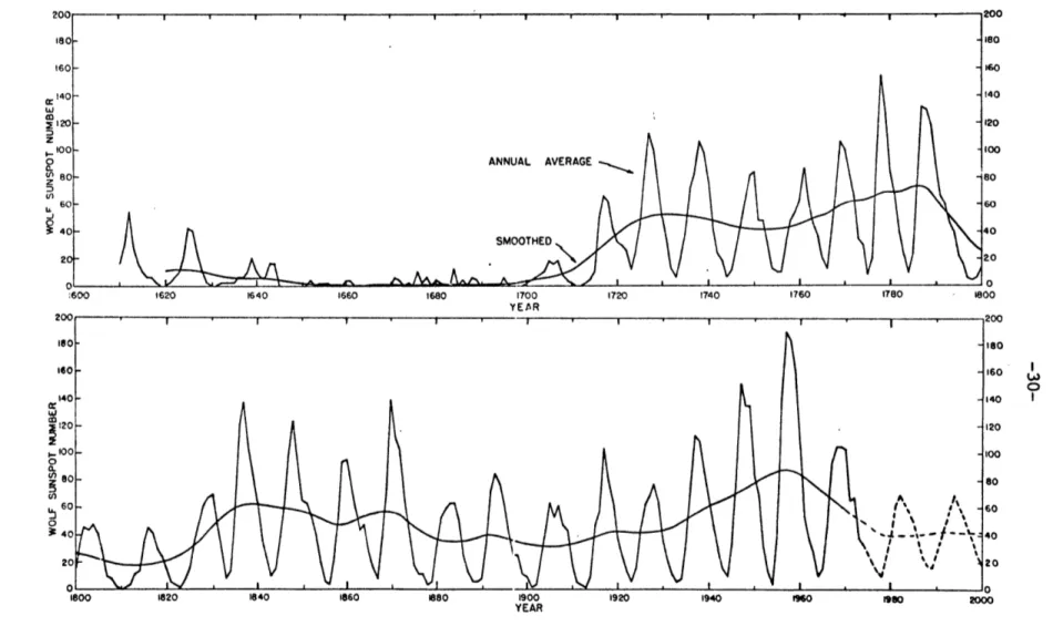
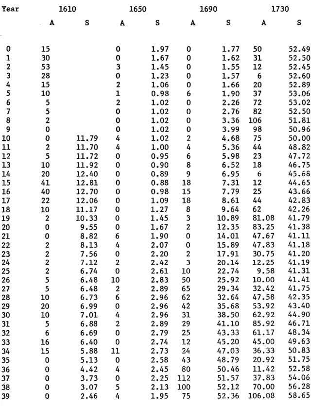
Counts of sunspots have been made since Galileo invented the telescope in 1610. Figure 7 is a graph of the Wolf sunspot number from

1610 to the present and also includes predictions by Sleeper (1975) to 1989 and by Willett (personal communication) until 2001. The numbers

for the 1600's and early 1700's are not as reliable as the later ones, and for the early 1600's are interpolated from the data of Eddy (1976). Table 1 contains the numbers used in the figure. The period from 1645

to 1715 is known as the Maunder minimum and was a period of very low sunspot activity. Since then the sunspot number has exhibited a rather regular variation with an 11-year period but variable amplitude. The predicted values of the Wolf number should be considered speculative. No skill has yet been demonstrated in forecasting the details of the sunspot cycle. The predictions are included for completeness, as

simu-lation runs with the model will be carried out to the year 2000.

Cohen and Lintz (1974) have performed a maximum entropy spectral analysis of the cycle and found periods of 90 and 11 years. Schove

(1955) found periods of 11 and 78 years. Sleeper (1972) and Gribbin (1973) have claimed that the gravitational field in the solar system,

mainly influenced by the orbits of Saturn and Jupiter, but also in accordance with the orbits of the minor planets, exhibits a 180-year periodicity with minor periods of 11 and 22 years, and with the

Figure 7. Graph of Wolf sunspot number, 1610-2001. See text for data sources.

t80

160

-31-Table 1. Wolf sunspot numbers, 1610 - 2001. Annual average (A) and smoothed (S) values are listed. See text for data sources.

Year 1610 1650 1690 1730 A S A S A S A S 0 15 0 1.97 0 1.77 50 52.49 1 30 0 1.67 0 1.62 31 52.50 2 53 3 1.45 0 1.55 12 52.45 3 28 0 1.23 0 1.57 6 52.60 4 15 2 1.06 0 1.66 20 52.89 5 10 1 0.98 6 1.90 37 53.06 6 5 2 1.02 0 2.26 72 53.02 7 5 0 1.02 0 2.76 82 52.50 8 2 0 1.02 0 3.36 106 51.81 9 0 0 1.02 0 3.99 98 50.96 10 0 11.79 4 1.02 2 4.68 75 50.00 11 2 11.70 4 1.00 4 5.36 44 48.82 12 5 11.72 0 0.95 6 5.98 23 47.72 13 10 11.92 0 0.90 8 6.52 18 46.75 14 20 12.40 0 0.89 9 6.95 6 45.68 15 41 12.81 0 0.88 18 7.31 12 44.65 16 40 12.70 0 0.98 15 7.79 25 43.66 17 22 12.06 0 1.09 18 8.61 44 42.83 18 10 11.17 0 1.27 8 9.64 62 42.26 19 2 10.33 0 1.45 3 10.89 81.08 41.79 20 0 9.55 0 1.67 2 12.35 83.25 41.38 21 0 8.82 6 1.90 0 14.01 47.67 41.11 22 2 8.13 4 2.07 0 15.89 47.83 41.18 23 2 7.56 0 2.20 2 17.91 30.75 41.20 24 2 7.12 2 2.42 3 20.14 12.25 41.19 25 2 6.74 0 2.61 10 22.74 9.58 41.31 26 5 6.48 10 2.83 50 25.92 10.00 41.41 27 5 6.48 2 2.89 65 29.34 32.42 41.75 28 10 6.73 6 2.96 62 32.64 47.58 42.35 29 20 6.99 0 2.96 42 35.68 53.92 43.40 30 10 7.01 4 2.96 31 38.50 62.92 44.90 31 5 6.88 2 2.89 29 41.10 85.92 46.71 32 6 6.69 0 2.79 25 43.33 61.17 48.34 33 16 6.40 0 2.74 12 45.20 45.00 49.63 34 15 5.88 11 2.73 24 47.03 36.33 50.83 35 0 5.13 0 2.58 43 48.79 20.92 51.75 36 0 4.42 4 2.45 80 50.46 11.42 52.58 37 0 3.73 0 2.25 112 51.57 37.83 54.06 38 0 3.07 5 2.13 100 52.12 70.00 56.28 2.46 4 1.95 75 52.36 106.08 58.65

39

0

Table 1. (continued) Year 1770 1810 1850 1890 A S A S A S A S 0 100.67 60.36 0.0 18.76 66.58 56.06 7.08 39.17 1 81.67 61.42 1.42 18.40 64.42 55.20 35.58 39.75 2 66.42 61.96 4.92 18.16 54.17 54.29 73.00 40.05 3 34.75 62.31 12.17 18.15 39.08 53.15 85.00 39.80 4 30.67 62.67 13.83 18.37 20.50 51.95 78.08 38.98 5 7.00 63.09 35.50 18.86 6.50 50.76 64.08 37.92 6 19.83 64.39 45.83 19.45 4.17 49.71 41.75 36.78 7 92.42 66.62 41.00 20.05 22.67 49.00 26.17 35.88 8 154.33 68.49 30.42 20.72 54.75 48.72 26.83 35.17 9 126.00 69.11 24.00 21.52 93.92 48.96 12.08 34.48 10 84.83 68.96 15.67 22.58 95.75 49.83 9.33 33.80 11 68.17 68.84 6.58 23.79 77.08 50.83 2.75 33.07 12 38.50 68.93 4.08 25.13 59.08 51.94 4.92 32.38 13 22.75 69.43 1.75 26.48 44.08 53.16 24.42 31.91 14 10.17 70.45 8.50 27.95 47.08 54.46 42.00 31.72 15 24.00 71.77 16.58 29.85 30.58 55.45 63.50 31.93 16 82.92 73.07 36.33 32.60 16.33 56.20 53.83 32.21 17 132.00 73.12 49.75 36.18 7.33 56.83 62.00 32.99 18 130.92 71.17 62.42 40.17 37.42 57.41 48.67 33.75 19 118.17 67.89 67.00 44.18 73.83 57.60 43.92 34.45 20 89.83 64.05 70.92 47.86 139.08 57.29 18.50 34.95 21 66.58 60.05 47.83 50.87 111.08 55.90 5.67 35.47 22 60.08 56.01 27.58 53.41 101.83 53.97 3.50 36.09 23 46.92 51.91 8.67 55.64 66.25 51.51 1.42 36.72 24 40.92 47.74 13.25 57.89 44.58 48.98 9.50 37.51 25 21.42 43.43 57.00 60.27 17.17 46.50 47.42 38.70 26 16.08 39.08 121.50 62.28 11.25 44.34 57.08 39.99 27 6.33 34.75 138.33 63.23 12.17 42.35 103.83 41.43 28 4.00 31.07 103.25 63.23 3.25 40.35 80.50 42.24 29 6.92 28.43 86.00 62.72 6.00 38.41 63.67 42.77 30 14.50 26.76 63.25 61.86 32.42 36.73 37.67 42.95 31 34.08 25.83 36.83 61.03 54.25 35.43 26.17 43.04 32 45.00 25.13 24.08 60.64 59.58 34.98 14.25 42.94 33 43.00 24.34 10.67 60.56 63.75 35.17 5.75 42.70 34 47.42 23.44 15.17 60.70 63.50 35.79 16.58 42.47 35 42.17 22.44 40.17 60.72 52.25 36.44 44.42 42.27 36 28.17 21.46 61.50 60.22 25.33 36.94 63.83 42.08 37 10.17 20.54 98.50 59.36 13.00 37.38 69.08 42.16 38 8.17 19.83 124.25 58.33 6.83 37.92 77.83 42.48 39 2.42 19.23 95.92 57.17 6.17 38.54 64.92 43.11

-Im'IlImIIEuImm.h, -33-Table 1. (continued) Year 1930 1970 A S A S 0 35.67 43.89 104.92 58.52 1 21.25 44.99 66.67 55.93 2 11.17 46.41 68.83 53.75 3 5.58 47.80 38.17 51.39 4 8.67 49.39 34 49.18 5 36.00 51.16 27 47.05 6 79.67 53.23 19 44.87 7 114.33 55.61 13 42.70 8 109.50 57.75 10 40.84 9 88.75 59.77 23 39.72 10 67.67 61.66 39 39.30 11 47.50 63.54 62 39.42 12 30.58 65.20 70 39.78 13 16.25 66.63 63 40.02 14 9.50 67.93 57 40.36 15 33.17 69.43 49 40.59 16 92.58 71.62 38 40.72 17 151.50 74.15 24 40.81 18 136.17 76.37 17 40.96 19 135.25 78.58 15 41.14 20 84.17 80.39 26 41.14 21 69.50 81.99 37 41.14 22 31.33 83.31 48 41.14 23 13.83 84.74 59 41.14 24 4.42 86.27 70 41.14 25 38.00 88.00 61 41.14 26 141.75 89.55 53 41.14 27 189.83 89.82 44 41.14 28 184.58 88.58 36 41.14 29 158.42 86.42 25 41.14 30 112.33 83.64 17 41.14 31 53.92 80.67 10 41.14 32 37.67 78.07 33 27.83 75.73 34 10.17 73.48 35 15.17 71.40 36 46.75 69.26 37 93.67 66.77 38 106.08 63.98 39 105.58 61.20

year period broken into 100- and 80-year periods. Willett (1974) uses all these periods, emphasizing the 22-year period, to find correlations with past climate change and make forecasts for the future. He points

out that during the first 11-year cycle of the double cycle sunspot pairs are led by spots of one polarity as they travel around the sun, and during the second cycle the polarity reverses. At the end of the

80- and 100-year portions of the 180-year cycle, the polarity does not

reverse between 11-year cycles. This conjecture, however, has yet to be observed. Sleeper (1974, 1975) uses these past variations to make forecasts into the future of the sunspot cycle.

To summarize, the sunspot number shows an obvious 11-year period-icity superimposed on what some have claimed are 22-, 80-, 100-, and 180-year periods. Yet during the Maunder minimum very few suaspots were observed. Observations of sunspots are quite good since 1750,

and fairly good from 1610 to 1750. Based on past periodicities, pre-dictions of the cycle have been made for 25 years into the future, but they must be considered speculative.

2) The longest series of observations of the solar constant were made by the Smithsonian Institution under the direction of Charles Greeley Abbott, from 1905 to 1952 (Abbot; 1963, 1966). During this period they made observations of the solar constant from the earth's surface, making theoretical and observational corrections for the

atmospheric attentuation of the solar radiation. The largest atmosphe-ric effects are due to the changing concentrations of water vapor and ozone. From 1905 to 1920 they spent about six months each year making observations from Mt. Wilson. Mountain top stations were used to lessen

lil i 1 I I

-35-the effects of -35-the atmosphere. Using Langley's "long method" -35-they cal-culated the solar constant. During the early 1920's a new "short

method" was devcloped to rapidly calculate the solar constant, and from

1923 to 1952 daily measurements were made from several mountain top

observatories in both the Northern and Southern Hemispheres.

Abbott claimed to have found a variation in the solar constant in phase with the 22 year, 9 month, double sunspot cycle with an amplitude of 3 %. He also claimed to have found 27 harmonics of this cycle, all with periods that are exact fractions of the basic 273 month period.

Later analysis of Abbott's data (Foukal et al., 1977) also showed a secular trend of 0.17 % during the 30 years that Abbott took his data, but found that this was probably due to changing calibration techniques, which overemphasized solar constant values that were high. The vali-dity of Abbott's results has been the subject of much criticism. The inexactness of the atmospheric corrections may have resulted in spurious values. Furthermore, changes in the observers and instruments over a 30-yea'r period probably introduced errors as large as the changes measured in the solar constant.

Kondratyev and Nikolsky (1970), from a series of about 8 balloon measurements made during the mid-1960's from altitudes of about 30 km, also measured large changes in the solar constant, and related them to the sunspot number by the empirical formula:

SC = 1.903 + 0.011 W.5 - 0.0006 W ly/min

where SC is the solar constant and W is the Wolf sunspot number. Yet their measurements were taken during a period of atmospheric nuclear

testing and injection into the stratosphere of large quantities of dust

by the eruption of Gunung Agung in Bali in 1963, and although they tried

to correct for these effects, their measurements are open to serious question, as they readily admit.

The problems of atmospheric effects associated with these attempts at measuring the solar constant strongly suggest that a better way would be measurements from satellites above the atmosphere. So far there has been no long-term program of measurement of the solar con-stant by satellite. This has been partially a problem of reliable instruments not being available that can maintain a calibration for a long time, and partially the lack of interest in, or realization of the importance of, or belief at all in, the variation of the solar constant

by NASA. But with the Space Shuttle to aid in the calibration and the

clamor for such measurements by people studying climate, a program such as this is sure to be started in the near future.

Three space vehicles launched by the United States have had instruments which measured the solar constant: Nimbus F and Mariner

6 and 7 (Foukal et al., 1977). Each of these had a large day to day instrumental drift of about 0.03 %/day so were useless for measuring long-term changes in the solar constant. Yet these data were useful in investigating short-term variations associated with sunspots and facu-lae. Foukal found a maximum variation of the solar constant of 0.03 % associated with magnetic solar variations, much less than that expected due to the darkening and brightening of the sun produced by the magnetic variations. He concluded that the darkness and brightness of sunspots

-37-Foukal also decided to search in Abbott's data for a variation in the solar constant associated with the maximum and minimum value of facular area and sunspot number during each month. He found no rela-tionship with sunspots, but did find an average 0.05 % variation in the solar constant from minimum to maximum facular area in each month. The average monthly facular area variation is half the average variation during a solar cycle, so Foukal concludes that there may be a 0.1 % var-iation in the surface observations of solar constant of Abbott, associa-ted with facular area changes, which correspond to the sunspot cycle. Since no such relationship was observed in the spacecraft data, he con-cludes that this must have been an atmospheric effect, most probably that of ozone, as discussed in the next section. Yet Abbott tried to correct his measurements for ozone variation! So Abbott's uncorrected values should show an even larger effect, of, at present, unknown mag-nitude.

Eddy (1976) as a result of his study of the Maunder minimum and

cosmic ray variation has theorized that there may be a long-term varia-tion of the solar constant that is unrelated to the variavaria-tions within each 11-year sunspot cycle. The magnitude of this solar constant change would be indicated by the overall envelope.of sunspot numbers, with the

11-year cycle filtered out. He supports this theory with the fact that this envelope was very low during the Maunder minimum, which correspon-ded to the Little Ice Age. An 11-year running mean was applied twice to the annual average sunspot data to produce a smoothed sunspot value to test this theory. The smoothed data are shown in Table 1 and Figure

7 with the annual average data.

3) Although changes in the solar constant related to the sunspot

cycle are very small, if they exist at all, changes in certain shortwave frequencies have been well documented and large. At 0.2 y there is a

1 % modulation in the solar flux by faculae and at smaller wavelengths,

the modulation can be more than ten times this effect (Foukal et al.,

1977). Less than 0.1 % of the energy of the total solar flux is in

wavelengths smaller than 0.2 p, but an indirect mechanism exists which may affect the amount of solar radiation reaching the surface. Ozone is created in the upper stratosphere at wavelengths between 0.18 and 0.21 V and Willett (1962) found a highly significant correlation between ozone concentration and the sunspot number. Ruderman and Chamberlain

(1975) point out that cosmic rays reaching the earth also vary with the

sunspot cycle, and that they affect the NO concentration. During sun-spot maximum, the cosmic rays are less, lowering the NO concentration,

x

which in turn lowers the catalytic destruction of ozone. These two mechanisms work together to increase the ozone concentration during sunspot maximum. The combined radiation effects of these ozone and NO

x changes have been studied by Ramanathan et al. (1976) with a

one-dimensional radiation model. They found that surface temperatures go up as ozone concentration goes up. The NO radiative effects partly

x

compensate for this temperature rise. Angione et al. (1976) also sug-gested that this variation of ozone causes ozone to act as a shutter,

modulating solar radiation by absorbing it in the Chappuis band (0.5

-0.7 P) in the center of the visible spectrum. The ozone observations

are not yet good enough and the above theoretical interactions are too poorly understood to indicate the magnitude of the total effect, but it

-39-could produce variations of sufficient magnitude to cause climate change.

The evidence therefore points to a possible indirect mechanism, through ozone, of a relationship between sunspot number, an indicator of faculae, and the amount of solar radiation reaching the ground. This effect was filtered out quite well by Abbott, so only a small sig-nal is detectable in his data, yet a much larger effect may exist.

4) One other short-term effect of the sun on the atmosphere has been well documented. It has been shown that the vorticity area index, a measure of the relative area of low pressure systems, is related, with a time lag, to passages of the earth through solar magnetic sector boundaries. This effect has been measured for the Northern Hemisphere only in the winter, when storms are strong. It has been documented by Schuurmans (1969), Roberts and Olson (1973), Hines and Halevy (1975), Wilcox (1976), Wilcox et al. (1976), and Shapiro (1976). No long-term effects have been measured, since passages of the magnetic sector boun-dary can only be measured by satellites above the atmosphere, and these measurements have only been made for a few years. It is interesting to note that McGuirk and Reiter (1976) have found a significant vacillation in atmospheric energy parameters with a mean period of about 24 days. This period is almost the same as that of the rotation of the sun. Al-though they did not mention the sun as a cause of the observed vacilla-tion, it may possibly be. Care should be taken not to make conclusions solely on the basis of similar periods, as this has been done

extensive-ly with 11-year periodicities observed on earth. A further study

rela-ting McGuirk and Reiter's parameters to the vorticity area index or to MIMI

magnetic sector boundary passages may prove fruitful.

5) It is conceivable that there may be variations in the solar

constant perceive~d at the earth's surface, probably through the ozone shutter mechanism. It is also conceivable that there may be a long-term drift in the solar constant related to the envelope of the sunspot number. Short-term variations of the weather may also be related to

the sun. All these theories will be tested by the model used in this thesis. Details of how they will be incorporated into the model will be discussed later, after the model is described.

One globally averaged model (Schneider and Mass, 1975) has been used to test the Kondratyev and Nikolsky theory, and got a large unreal

11-year cycle in predicted temperature. For more details see section II.D.3.

b. Volcanic dust

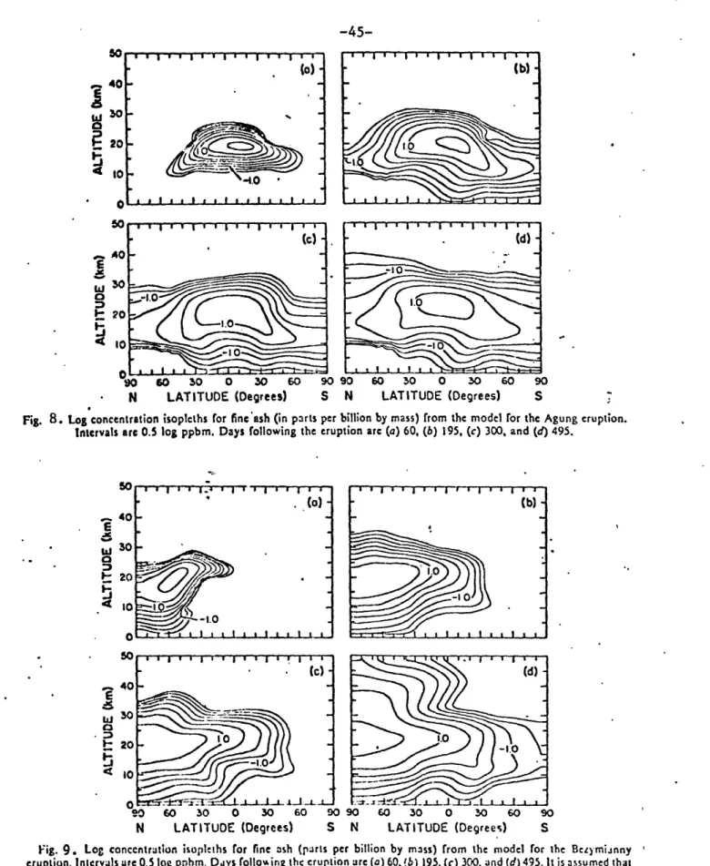
When large volcanoes erupt, they inject aerosol particles into the stratosphere. These particles interact with radiation in the atmosphere with the net effect of blocking some of the solar radiation and cooling the earth. Newell and Weare (1976) have shown that the eruption of Gunung Agung in Bali in March, 1963, produced a temporary

0.5*C cooling of the tropical troposphere. Dyer (1974) also studied

the Agung eruption and showed that its effects disappeared after 8

years. Thus volcanoes produce climate changes of a time scale important to the subject of this thesis. Periods of increased volcanism may have produced climate change on ice-age time scales also. Ninkovitch and Donn (1976) have studied ocean cores and have concluded that there is

-41-still not enough evidence at this time to determine whether long

enough periods of increased volcanism existed to modify climate. Roosen et al. (1976), however, claim to have found a relation between earth tides, volcanism and the temperature record of the Greenland ice cores to explain part of the ice-age temperature change. Bray (1974, 1976) also claims to have found evidence that ice-age glacial advances were synchronous with periods of increased volcanism. In any case, if it can be shown that volcanoes do produce cooling, even though volcanic eruptions cannot at this time be forecast, a massive eruption could be used to forecast climate change for the succeeding 10 years.

Lamb (1970) has compiled a list of volcanic eruptions since the year 1500. The evidence for the earlier of these is based on anecdotal historical records and as such is not very reliable. Also, records for the Southern Hemisphere do not exist until the nineteenth century. Nevertheless, Lamb has assigned magnitudes to the various eruptions and indicated the relative effect each would have on the Northern and

Southern Hemispheres. His volcanic dust veil index (Table 2) is his estimate of the relative stratospheric dust load produced by volcanoes for the Northern Hemisphere for each year since 1600. The values in

1975-1978 were added to account for the Fuego eruption. Russell and

Hake (1977) have shown that this dust veil was less extensive than that of Agung in Central America. Mitchell (1970) has used Lamb's raw data to produce his own estimate of the global dust load for 1850 to the present (Table 3). He also includes eruptions during the present cen-tury that Lamb excluded as being too small, and therefore his record is more detailed and accurate. One must be careful when using this data as