Closed-forms of Kirchhoff elastic rods shape and sensitivity in the planar case

(1)

HAL Id: hal-01133395

https://hal.archives-ouvertes.fr/hal-01133395v3

Submitted on 7 Apr 2015

HAL is a multi-disciplinary open access

archive for the deposit and dissemination of

sci-entific research documents, whether they are

pub-lished or not. The documents may come from

teaching and research institutions in France or

abroad, or from public or private research centers.

L’archive ouverte pluridisciplinaire HAL, est

destinée au dépôt et à la diffusion de documents

scientifiques de niveau recherche, publiés ou non,

émanant des établissements d’enseignement et de

recherche français ou étrangers, des laboratoires

publics ou privés.

Distributed under a Creative Commons Attribution - ShareAlike| 4.0 International

License

Closed-forms of Kirchhoff elastic rods shape and

sensitivity in the planar case

Olivier Roussel, Marc Renaud, Michel Taïx

To cite this version:

Olivier Roussel, Marc Renaud, Michel Taïx. Closed-forms of Kirchhoff elastic rods shape and

sensi-tivity in the planar case. [Research Report] LAAS-CNRS. 2015. �hal-01133395v3�

(2)

Closed-forms of Kirchhoff elastic rods shape and

sensitivity in the planar case

Olivier Roussel

1

, Marc Renaud

1

and Michel Ta¨ıx

1˚

Abstract

In this report we give closed-forms of Kirchhoff 3-D elastic rods curvature in terms of elliptic functions and, by treating planar rods as a special case, we show we can also obtain closed-forms of planar rods shape, sensitivity and total elastic energy.

1 General case of 3-D rods

Consider an inextensible, non-shearable and unit length linearly elastic rod. The shape of the rod traces a curve that we will describe by the mapping q : r0, 1s Ñ SEp3q. The position along the rod is parametrized by t P r0, 1s and we will name ”base” and ”tip” of the rod its extremity at t “ 0 and t “ 1 respectively. Let the mappings u1ptq, u2ptq, u3ptq such that ui: r0, 1s Ñ R be

axial and bending rod strains respectively, and c1, c2, c3be the constants that reflect its elasticity

properties. As in [3], we say the elastic rod is in static equilibrium in the sense of Kirchhoff if it locally minimizes the elastic energy defined by

Eel “ 1 2 ż1 0 3 ÿ i“1 ciu2i dt. (1.1)

Without loss of generality, we will also assume that the base of the rod is held fixed at the origin, i.e. qp0q “ e where e is the identity element of SEp3q. Under these assumptions, we will denote by B the set of positions that the other extremity of the rod qp1q can reach. As shown in [2], the problem of static equilibrium of such rods can be formulated as an optimal control problem by minimize q,u 1 2 ż1 0 3 ÿ i“1 ciu2i dt subject to q “ q9 ˜ ₃ ÿ i“1 uiXi` X4 ¸ qp0q “ e, qp1q “ b (1.2)

for some b P B and where X1“ „_{0 0 0 0} 0 0 ´1 0 0 1 0 0 0 0 0 0  X2“ „ _{0 0 1 0} 0 0 0 0 ´1 0 0 0 0 0 0 0  X3“ „_{0 ´1 0 0} 1 0 0 0 0 0 0 0 0 0 0 0  X4“ „_{0 0 0 1} 0 0 0 0 0 0 0 0 0 0 0 0  X5“ „_{0 0 0 0} 0 0 0 1 0 0 0 0 0 0 0 0  X6“ „_{0 0 0 0} 0 0 0 0 0 0 0 1 0 0 0 0 

is a basis for sep3q, the Lie algebra of SEp3q. Note that when solving this optimal control problem, the rod tip position b is not an input.

(3)

In these conditions, the Maximum Principle states that solutions to this optimal control problem are the projections of extremal curves defined on the cotangent bundle T˚_{SEp3q onto}

SEp3q. Thanks to the Lie Group structure of SEp3q, the Hamiltonian can be reduced on the dual of the Lie algebra sep3q˚_{and the corresponding (time-varying) Hamiltonian vector fields}

µ : r0, 1s Ñ sep3q˚_{can be expressed by}

$ ’ ’ ’ ’ ’ ’ ’ & ’ ’ ’ ’ ’ ’ ’ % 9 µ1“µ3_cµ2 3 ´ µ2µ3 c2 9 µ2“ µ6`µ1cµ13 ´ µ1µ3 c3 9 µ3“ ´µ5`µ_c1µ₂2 ´µ1_cµ₁2 9 µ4“µ3_cµ₃5 ´µ2_cµ₂6 9 µ5“µ1_cµ6 1 ´ µ3µ4 c3 9 µ6“µ2_cµ4 2 ´ µ1µ5 c1 (1.3)

where vector fields µ are related to controls uiby ui“ c´1i µifor i P t1, 2, 3u.

Let A be the set homeomorphic to R6and a P A such that aifi µip0q, i P t1, . . . , 6u. It has

been shown in [2] that coordinates in A offer a global parameterization to the set of static equi-librium configuration for the rod. In other words, we can describe configurations of quasi-static 3-D elastic rods using the 6-dimensional configuration space A.

Assuming isotropy and normalized elasticity constants such that ci “ 1 for i P t1, 2, 3u, we

have from (1.3) 9µ1“ 0. Then µ1is a constant of motion with µ1“ a1and

$ ’ ’ ’ ’ & ’ ’ ’ ’ % 9 µ2“ µ6 9 µ3“ ´µ5 9 µ4“ µ3µ5´ µ2µ6 9 µ5“ a1µ6´ µ3µ4 9 µ6“ µ2µ4´ a1µ5 (1.4)

The signed curvature κ and the torsion τ of the curve can be expressed in terms of µ by κ2“ µ22` µ 2 3 τ “ µ1´ µ2µ5` µ3µ6 µ2 2` µ23

and, as mentioned in [2], the differential system (1.4) is equivalent to

2:κ ` κ3´ 2κpτ ´ λ1q2“ λ2κ (1.5a)

κ2pτ ´ λ1q “ λ3 (1.5b)

where the constants of integration are given by $ & % λ1fi a₂1 λ2fi a22` a 2 3` 2a4´ a2 1 2 λ3fi a₂1pa22` a23q ´ pa2a5` a3a6q.

Substituting (1.5b) into (1.5a) and integrating, we obtain 9 κ2`1 4κ 4 ` λ23κ´2´ λ2 2 κ 2 “ λ4 (1.6)

where the constant of integration λ4is given by

λ4fi a25` a 2 6´ 1 4pa 2 2` a 2 3q 2 `1 2pa 2 2` a 2 3qpa 2 1´ 2a4q ´ a1pa2a5` a3a6q

By making the change of variable υ “ κ2_{, (1.6) transforms to}

9

(4)

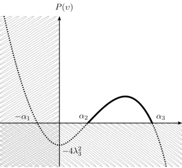
Figure 1: Plot of the cubic polynomial P pυq with respect to the squared curvature υ. Hatched regions correspond to impossible values illustrating that the only valid range for υ is given by α2and α3, the zeros of P pυq.

As already stated in [4], this equation is in the form 9υ2

“ P pυq with P is the cubic polynomial P pυq fi ´υ3` 2λ2υ2` 4λ4υ ´ 4λ23. (1.8)

Let ´α1, α2, α3be the zeros of the polynomial P pυq such that

´α1ď 0 ď α2ď α3. (1.9)

.

As P p˘8q “ ¯8 and P p0q “ ´4λ23ď 0, P pυq is in the form illustrated in figure 1.

Also, we have υ ě 0 and P pυq ě 0 as they are both squares, so υ P rα2, α3s.

The polynomial P pυq can be rewritten for its zeros by

P pυq “ ´pυ ` α1qpυ ´ α2qpυ ´ α3q.

We can express the polynomial zeros ´α1, α2, α3from the constants of integrations λiby

α1´ α2´ α3 “ ´2λ2

α1α2` α1α3´ α2α3 “ 4λ4

α1α2α3 “ 4λ23.

(1.10)

The squared curvature υ can be expressed in terms of elliptic functions by υptq “ α3

´

1 ´ n sn2`rt ` ϕ|m˘ ¯

(1.11) the parameter m, the characteristic n and r can be expressed from the polynomial zeros by

m “α3´ α2 α3` α1 n “ α3´ α2 α3 r “ 1 2 ? α3` α1 (1.12)

(5)

Given $ fi d 1 n ˆ 1 ´ a 2 2` a23 α3 ˙ (1.13)

the phase ϕ can be retrieved from a2₂` a2₃“ α3`1 ´ n sn2pϕ|mq

˘

, and is given by

ϕ “ sgnpa3a5´ a2a6q arcsnp$|mq (1.14)

where arcsn is the inverse of the Jacobi elliptic function sn. Note that from (1.9), we have 0 ď m ď n ď 1.

As outlined in [3], it has been shown the Hamiltonian vector fields in (1.4) is integrable and we have proved it can be expressed in the following form

$ ’ ’ ’ ’ ’ & ’ ’ ’ ’ ’ % µ2“ κ sin ψ µ3“ κ cos ψ µ4“ 1₂pλ2` a2₁ 2 ´ υq µ5“ ´ 9κ cos ψ ` κ 9ψ sin ψ µ6“ 9κ sin ψ ` κ 9ψ cos ψ. (1.15) where ψptq “ λ1t ´ λ3 α3r ˆ Π ´ n, am`rt ` ϕ|m˘|m ¯ ´ Π ´ n, am`ϕ|m˘|m ¯˙ ` ψ p0q

with Πpn, u|mq the elliptic integral of the third kind and ampu|mq is the Jacobi amplitude.

2 Planar case

Although neither the curve qptq nor the rod sensitivity Bqptq_Ba can be explicitly expressed in the general 3-D case, we will show in this section that closed forms can be obtained in the planar case which can be treated as a particular case of the previously presented model.

2.1 Curvature and internal wrenches

Considering only planar curves qptq in the xy-plane with q “ p0, 0, θ, x, y, 0qT_{, Hamiltonian}

vector fields defined in (1.3) simplify to $ ’ ’ ’ ’ ’ ’ & ’ ’ ’ ’ ’ ’ % 9 µ1“ 0 9 µ2“ 0 9 µ3“ ´µ5 9 µ4“ µ3µ5 9 µ5“ ´µ3µ4 9 µ6“ 0 (2.1)

Closed-forms of rod internal wrenches µptq defined in (1.15) reduce to $ ’ ’ ’ ’ ’ ’ & ’ ’ ’ ’ ’ ’ % µ1“ 0 µ2“ 0 µ3“ κ µ4“ ´1₂pκ2` λ2q µ5“ ´ 9κ µ6“ 0 (2.2)

(6)

And constants of integration defined in (1) simplify to $ ’ ’ & ’ ’ % λ1“ 0 λ2“ a23` 2a4 λ3“ 0 λ4“ a25´ a23p14a 2 3` a4q

We retrieve the same results as we would have obtain by applying the same problem formu-lation on the Lie Group SEp2q rather than SEp3q. Therefore, in the rest of this section we will restrict to solutions of (1.2) that are similar to trajectories on SEp2q, which are generated by the subset of initial conditions ta P A : pa1, a2, a6q “ p0, 0, 0qu.

In the following equations, when referring to an elliptic function pq, we will simplify the notation pqpu|mq to pq u. Also, let us define

Γptq fi rt ` ϕ

and the following constants of motion that be needed in the following developments ε fi sgnpa3q

Γ0fi Γp0q

δ fi λ22` 4λ4

The expression of the phase ϕ given in (1.14) simplifies to ϕ “ sgnpa3a5q arcsnp$|mq

where $ given in (1.13) reduces to

$ “ d 1 n ˆ 1 ´ a 2 3 α3 ˙ .

2.1.1 Expression of the curvature

In the planar case, as λ3“ 0, the polynomial P pυq simplifies to

P pυq “ ´υ3` 2λ2υ2` 4λ4υ

so P pυq has one trivial zero at υ “ 0.

From (1.9), we can distinguish three cases as outlined in [4] and [5]: • Case I: λ4ą 0

Using (1.10), we have that

λ1pλ2` λ3q ą λ2λ3.

This imposes the choice for the zeros to $ & % α1“ ´λ2` ? δ α2“ 0 α3“ λ2` ? δ.

From (1.12) we get n “ 1, so the squared curvature formula in (1.11) simplifies to υptq “ α3`1 ´ sn2Γptq

˘ “ α3cn2Γptq.

(7)

Then the signed curvature is given by

κptq “ ε?α3cn Γptq. (2.3)

The curvature κptq oscillates between ?α3 and ´

?

α3 and the resulting curve qptq is

called a ”wavelike” elastica.

• Case II: λ4ă 0 Using (1.10), we have

λ1pλ2` λ3q ă λ2λ3.

This imposes the choice for the zeros to $ & % α1 “ 0 α2 “ λ2´ ? δ α3 “ λ2` ? δ.

From (1.12) we get n “ m, so the squared curvature formula in (1.11) simplifies to υptq “ α3`1 ´ m sn2Γptq

˘ “ α3dn2Γptq.

Then the signed curvature is given by

κptq “ ε?α3dn Γptq (2.4)

The curvature κptq is non-vanishing and the resulting curve qptq is called a ”orbit-like” elastica.

• Case III: λ4“ 0 This borderline case implies the polynomial P pυq reduces to

P pυq “ ´υ3` 2λ2υ2

which has a double zero.

Using first equation of (1.10), only one choice is possible for the zeros αi:

"

α1“ α2“ 0

α3“ |2λ2| .

which leads to the signed curvature

κptq “ ε?α3sech Γptq (2.5)

This corresponds to the borderline case where the curvature is non-periodic.

2.1.2 Reduction to a unique formulation of the curvature

These cases can be reduced to a single formulation of the curvature by allowing the parameter m to be any positive or null real and applying the Jacobi’s real transformation (see [1] §16.11). By relaxing the constraint on the zeros αigiven in (1.9), and keeping only one fixed choice on

(8)

$ & % α1 1“ 0 α1 2“ λ2´ ? δ α1 3“ λ2` ? δ. In this form, α1 3is positive as ?

δ ą |λ2| but α12can now be negative. Note that we still have

α1 3ě α12.

Using same forms as in (1.12), the elliptic parameter m1_{and r}1_by

m1 “ α 1 3´ α12 α1 3 r1 “1 2 a α1 3

but as mentioned before, the new elliptic parameter m1 _{is only constrained to in r0, 8q.}

Then, the signed curvature can be expressed by a unique expression by κptq “ εaα1

3dn`r1pt ` φq

ˇ ˇm1˘

(2.6) When m1 _{ą 1, the Jacobi’s real transformation can be applied to reduce to a parameter m}

such that 0 ď m ď 1 and we retrieve the previously described cases.

2.1.3 Explicit formulation of rod total elastic energy Recall from (1.1) the total elastic energy of the rod is given by

Eel“ 1 2 ż1 0 u3ptq2dt “ 1 2 ż1 0 κptq2dt

Using the unique formulation of the curvature κptq given in (2.6) can be integrated to give an explicit formulation in terms of the elliptic integral of the second kind by

Eel“ α1 3 2 E`r 1 pt ` φqˇˇm1˘

2.2 Integration of the curve qptq

From the differential system defined in (1.2), it follows that 9

θ “ u3“ κ x “ cos θ9 y “ cos θ.9

Using (2.2), the integration of the curvature is given by

cos θptq “ β1p0qβ1ptq ` 4β2p0qβ2ptq (2.7a) sin θptq “ 2 ε pβ1p0qβ2ptq ´ β2p0qβ1ptqq (2.7b) xptq “ β1p0q ż β1ptq ` 4β2p0q ż β2ptq (2.7c) yptq “ 2 ε ˆ β1p0q ż β2ptq ´ β2p0q ż β1ptq ˙ . (2.7d)

The functions β1ptq and β2ptq can be explicitly given using Jacobi elliptic functions and the

(9)

• Case I: λ4ą 0

Integrating the curvature in (2.3) (see [1] §16.24) leads to

θptq “ 2 ε parccos pdn Γptqq ´ arccos pdn Γ0qq

Let Aptq fi arccos pdn Γptqq and Ap0q fi arccos pdn Γ0q, then

cos Aptq “ dn Γptq sin Aptq “ ˘

b

1 ´ dn2Γptq “?m sn Γptq Given that θptq₂ “ ε pAptq ´ Ap0qq, we have

cosθptq

2 “ cos Aptq cos Ap0q ` sin Aptq sin Ap0q “ dn Γptq dn Γ0` m sn Γptq sn Γ0

sinθptq

2 “ sin Aptq cos Ap0q ´ cos Aptq sin Ap0q “ ε?m psn Γptq dn Γ0´ sn Γ0dn Γptqq

Using half-angle formulas, we get cos θptq “ cos2θptq 2 ´ sin 2θptq 2 “`2 dn2Γ0´ 1˘ `2 dn2Γptq ´ 1 ˘ ` 4m dn Γptq sn Γptq dn Γ0sn Γ0 sin θptq “ 2 cosθptq 2 sin θptq 2 “ 2 ε?m``2 dn2Γ0´ 1˘ dn Γptq sn Γptq ´ `2 dn2Γptq ´ 1˘ dn Γ0sn Γ0 ˘ which is in the form (2.7) with β1and β2given by

β1ptq fi 2 dn2Γptq ´ 1 (2.8a)

β2ptq fi

?

m sn Γptq dn Γptq (2.8b) and can be integrated to

ż

β1ptq “ 2r´1pEpam Γptqq ´ Epam Γ0qq ´ t (2.9a)

ż

β2ptq “ ´r´1pcn Γptq ´ cn Γ0q (2.9b)

(2.9c) • Case II: λ4ă 0

θptq “ 2 ε parcsin psn Γptqq ´ arcsin psn Γ0qq

Let Aptq fi arcsin psn Γptqq and Ap0q fi arcsin psn Γ0q, then

cos Aptq “ ˘a1 ´ sn2_Γptq

“ cn Γptq sin Aptq “ sn Γptq

(10)

Given that θptq₂ “ ε pAptq ´ Ap0qq, we have

cosθptq

2 “ cos Aptq cos Ap0q ` sin Aptq sin Ap0q “ cn Γptq cn Γ0` sn Γptq sn Γ0

sinθptq

2 “ sin Aptq cos Ap0q ´ cos Aptq sin Ap0q “ ε psn Γptq cn Γ0´ cn Γ0sn Γptqq

Using half-angle formulas, we get cos θptq “ cos2θptq 2 ´ sin 2θptq 2 “`1 ´ 2 dn2Γptq˘ `1 ´ 2 dn2Γ0 ˘ ` 4 cn Γptq sn Γptq cn Γ0sn Γ0 sin θptq “ 2 cosθptq 2 sin θptq 2 “ 2ε``1 ´ 2 sn2Γ0˘ cn Γptq sn Γptq ´ `1 ´ 2 dn2Γptq˘ cn Γ0sn Γ0 ˘ which is in the form (2.7) with β1and β2given by

β1ptq fi 1 ´ 2 sn2Γptq (2.10a)

β2ptq fi sn Γptq cn Γptq (2.10b)

and can be integrated to ż β1ptq “ m´1`t pm ´ 2q ` 2r´1pE pam Γ ptqq ´ E pam Γ0qq ˘ (2.11a) ż β2ptq “ ´r´1pcn Γptq ´ cn Γ0q (2.11b) (2.11c) • Case III: λ4“ 0

θptq “ 2 ε parctan psinh Γptqq ´ arctan psinh Γ0qq

Let Aptq fi arctan psinh Γptqq and Ap0q fi arctan psinh Γ0q, then

cos Aptq “ ˘`1 ` sinh2Γptq˘´

1 2

“ sech Γptq sin Aptq “ tanh Γptq

Given that θptq₂ “ ε pAptq ´ Ap0qq, we have

cosθptq

2 “ cos Aptq cos Ap0q ` sin Aptq sin Ap0q “ sech Γptq sech Γ0` tanh Γptq tanh Γ0

sinθptq

2 “ sin Aptq cos Ap0q ´ cos Aptq sin Ap0q “ ε ptanh Γptq sech Γ0´ tanh Γ0sech Γptqq

(11)

Using half-angle formulas, we get cos θptq “ cos2θptq 2 ´ sin 2θptq 2 “`2 sech2Γptq ´ 1˘ `2 sech2Γ0´ 1 ˘

` 4 sech Γptq tanh Γptq sech Γ0tanh Γ0

sin θptq “ 2 cosθptq 2 sin

θptq 2

“ 2 ε``2 sech2Γ0´ 1˘ sech Γptq tanh Γptq ´ `2 sech2Γptq ´ 1˘ sech Γ0tanh Γ0

˘ which is in the form (2.7) with β1and β2given by

β1ptq fi 2 sech2Γptq ´ 1 (2.12a)

β2ptq fi sech Γptq tanh Γptq (2.12b)

which integrate to ż

β1ptq “ 2r´1ptanh Γptq ´ tanh Γ0q ´ t (2.13a)

ż

β2ptq “ ´r´1psech Γ ptq ´ sech Γ0q . (2.13b)

2.3 Explicit formulation of elastic rod sensitivity

In the 3-D case, the elastic rod sensitivity is given by the 6-dimensional Jacobian matrix

Jpt, aq “ ¨ ˚ ˝ Bq1 Ba1 ¨ ¨ ¨ Bq1 Ba6 .. . . .. ... Bq6 Ba1 ¨ ¨ ¨ Bq6 Ba6 ˛ ‹ ‚ (2.14)

In the planar case, this simplifies to

Jpt, aq “ ¨ ˝ ˚2,2 02,3 ˚2,1 03,2 JP3,3pt, aq 03,1 ˚1,2 01,3 ˚1,1 ˛ ‚ (2.15)

where ˚ represents indeterminate values.

As we can only obtain closed-forms of the rod shape and thus of rod sensitivity in this special, we will focus in this section on the 3-dimensional block JP

pt, aq of Jpt, aq for i, j P t3, 4, 5u. Differentiating the general form of the curve qptq in (2.7)leads to

B cospθptqq Ba “ β1p0q Bβ1ptq Ba ` Bβ1p0q Ba β1ptq ` 4 ˆ β2p0q Bβ2ptq Ba ` Bβ2p0q Ba β2ptq ˙ (2.16a) B sinpθptqq Ba “ 2 ε ˆ β1p0q Bβ2ptq Ba ` β2ptq Bβ1p0q Ba ´ β2p0q Bβ1ptq Ba ´ β1ptq Bβ2p0q Ba ˙ (2.16b) Bxptq Ba “ β1p0q Bş β1ptq Ba ` ż β1ptq Bβ1p0q Ba ` 4 ˆ β2p0q Bş β2ptq Ba ` ż β2ptq Bş β2p0q Ba ˙ (2.16c) Byptq Ba “ 2 ε ˆ β1p0q Bş β2ptq Ba ` ż β2ptq Bβ1p0q Ba ´ β2p0q Bş β1ptq Ba ´ ż β1ptq Bş β2p0q Ba ˙ (2.16d) Regardless the three cases of curve elastica, we can derivate with respect to a the following forms:

(12)

• The elliptic parameters m, n and r Bm Ba “ 1 pα3` α1q2 ˆˆ Bα3 Ba ´ Bα2 Ba ˙ pα3` α1q ´ ˆ Bα3 Ba ` Bα1 Ba ˙ pα3´ α2q ˙ (2.17a) Br Ba“ 1 4?α3` α1 ˆ Bα3 Ba ` Bα1 Ba ˙ (2.17b) Bn Ba “ 1 α2 3 ˆ Bα3 Ba α2´ Bα2 Baα3 ˙ (2.17c) • The phase ϕ Given B$ Ba “ 1 2n$ ¨ ˚ ˚ ˝ a23 α2 3 ¨ ˚ ˚ ˝ Bα3 Ba3 ´ 2 α3 a3 Bα3 Ba4 Bα3 Ba5 ˛ ‹ ‹ ‚ ´1 n ˆ 1 ´ a 2 3 α3 ˙ Bn Ba ˛ ‹ ‹ ‚ (2.18)

and the first order derivatives of the function arcsnpz|mq B arcsnpz|mq Bz “ 1 ? 1 ´ z2?_{1 ´ mz}2 B arcsnpz|mq Bm “ 1 2 pm ´ 1q m ˆ m?1 ´ z2_z ? 1 ´ mz2 ´ Eparcsin z|mq ´ pm ´ 1q Fparcsin z|mq ˙

with cdpz|mq is the Jacobi elliptic function defined by cd z “ cn z

dn z,

we can express the derivative of the function arcsnp$|mq with respect to a using the chain rule B arcsn $ Ba “ B arcsn $ B$ B$ Ba ` B arcsn $ Bm Bm Ba “? 1 1 ´ mz2 ˆ 1 ? 1 ´ z2 B$ Ba ` mz?1 ´ z2_{´ Eparcsin $q ´ pm ´ 1q Fparcsin $q} 2pm ´ 1qm Bm Ba ˙

Then, the general expression of the derivative of the phase ϕ with respect to a is Bϕ Ba “ sgnpa3a5q B arcsnp$|mq Ba • The function Γptq BΓptq Ba “ t Br Ba` Bϕ Ba • The Jacobi elliptic function sn pΓptq|mq

(13)

we can compute directly B sn Γptq Ba “ B sn Γptq BΓptq BΓptq Ba ` B sn Γptq Bm Bm Ba “ cn Γptq dn Γptq ˆ BΓptq Ba ` pm ´ 1qΓptq ` Epam Γptqq ´ m cd Γptq sn Γptq 2mpm ´ 1q Bm Ba ˙ .

• The Jacobi elliptic function cn pΓptq|mq

we can compute directly B cn Γptq Ba “ B cn Γptq BΓptq BΓptq Ba ` B cn Γptq Bm Bm Ba “ ´ sn Γptq dn Γptq ˆ BΓptq Ba ` pm ´ 1qΓptq ` Epam Γptqq ´ m cd Γptq sn Γptq 2mpm ´ 1q Bm Ba ˙ .

• The Jacobi elliptic function dn pΓptq|mq

with scpz|mq is the Jacobi elliptic function defined by sc z “ sn z

cn z, we can compute directly

B dn Γptq Ba “ B dn Γptq BΓptq BΓptq Ba ` B dn Γptq Bm Bm Ba “ ´m cn Γptq sn Γptq ˆ BΓptq Ba ` pm ´ 1qΓptq ` m Epam Γptqq ´ m dn Γptq sc Γptq 2mpm ´ 1q Bm Ba ˙ .

• The elliptic integral of the second kind E pampΓptq|mq|mq

We first need to express the derivative of the amplitude ampΓptq|mq with respect to a. Given first derivatives of the Jacobi amplitude ampz|mq

(14)

we get the derivative of ampΓptq|mq with respect to a by applying the chain rule as usual B am Γptq Ba “ B am Γptq BΓptq BΓptq Ba ` B am Γptq Bm Bm Ba “ dn Γptq ˆ BΓptq Ba ` pm ´ 1qΓptq ` Epam Γptqq ´ m cd Γptq sn Γptq 2mpm ´ 1q Bm Ba ˙ .

B E pam Γptqq B am Γptq “ b 1 ´ m sin2pam Γptqq “a1 ´ sn2_Γptq “ dn Γptq, and that Fpam Γptqq “ Γptq,

we finally have all the expressions to compute the derivative of E pam Γptqq with respect to a by applying the chain rule

B E pam Γptqq Ba “ B E pam Γptqq B am Γptq B am Γptq Ba ` B E pam Γptqq Bm Bm Ba “ dn2Γptq ˆ BΓptq Ba ` Epam Γptqq ´ cd Γptq sn Γptq 2pm ´ 1q Bm Ba ˙

Then, most of these forms simplify in the three previously introduced cases and we can give the explicit forms of the derivatives of functions β1ptq and β2ptq (and their respective integrals)

with respect to a: • Case I: λ4ą 0

From (2.8) and (2.9), we get Bβ1ptq Ba “ 4 dn Γptq B dn Γptq Ba Bβ2ptq Ba “ dn Γptq B sn Γptq Ba ` sn Γptq B dn Γptq Ba Bş β1ptq Ba “ 2 r ˆˆ B EpΓptqq Ba ´ B EpΓ0q Ba ˙ ´1 r ´ EpΓptqq ´ EpΓ0q ¯_Br Ba ˙ Bş β2ptq Ba “ 1 r ˆ 1 rpcn Γptq ´ cn Γ0q Br Ba´ ˆ B cn Γptq Ba ´ B cn Γ0 Ba ˙˙ • Case II: λ4ă 0

(15)

From (2.10) and (2.11), we get Bβ1ptq Ba “ ´4 sn Γptq B sn Γptq Ba Bβ2ptq Ba “ cn Γptq B sn Γptq Ba ` sn Γptq B cn Γptq Ba Bş β1ptq Ba “ 1 m ˆ tp1 ´ mq m Bm Ba ` 2 rpEpam Γptqq ´ Epam Γ0qq ˆ 1 r Br Ba´ 1 m Bm Ba ˙ `2 r ˆ B EpΓptqq Ba ´ B EpΓ0q Ba ˙˙ Bş β2ptq Ba “ 1 rm ˆ pdn Γptq ´ dn Γ0q ˆ 1 m Bm Ba ` 1 r Br Ba ˙ ´ ˆ B dn Γptq Ba ´ B dn Γ0 Ba ˙˙ • Case III: λ4“ 0

From (2.12) and (2.13), we get Bβ1ptq Ba “ ´2 sech 2 Γptq tanh Γptq Bβ2ptq Ba “ sech Γptq`1 ´ 2 tanh 2 Γptq˘ Bş β1ptq Ba “ 2 r ˆ 1 r Br

Baptanh Γptq ´ tanh Γ0q ´`tanh

2 Γptq ´ tanh2Γ0 ˘ ˙ Bş β2ptq Ba “ 1 r ˆ

tanh Γptq sech Γptq ´ tanh Γ0sech Γ0´

1

rpsech Γptq ´ sech Γ0q ˙

Acknowledgments

This work was supported by the French National Research Agency under the project Flecto (ANR- Digital Models).

References

[1] M. Abramowitz and I. Stegun. Handbook of Mathematical Functions. Dover, 1964. [2] T. Bretl and Z. McCarthy. Quasi-static manipulation of a kirchhoff elastic rod based on a

geometric analysis of equilibrium configurations. I. J. Robotic Res., 33(1):48–68, 2014. [3] V. Jurdjevic. Integrable Hamiltonian systems on complex Lie groups. Memoirs of the

American Mathematical Society. 2005.

[4] J. Langer and D. A. Singer. The total squared curvature of closed curves. J. Differential Geom., 20(1):1–22, 1984.