Cognitive Information Processing

(1)

XII. COGNITIVE INFORMATION PROCESSING

Academic and Research Staff

Prof. W. L. Black Prof. W. F. Schreiber Dr. P. H. Liss Prof. M. Eden Prof. D. E. Troxel Dr. O. J. Tretiak Prof. T. S. Huang Dr. K. R. Ingham C. L. Fontaine Prof. F. F. Lee Dr. P. A. Kolers E. R. Jensen

Prof. S. J. Mason G. L. Wickelgren

Graduate Students

G. B. Anderson D. W. Hartman G. F. Pfister T. P. Barnwell III H. P. Hartmann D. S. Prerau

B. A. Blesser G. R. Kalan G. M. Robbins

A. L. Citron R. W. Kinsley, Jr. C. L. Seitz

D. P. De Wan W. H. Lee D. Sheena

H. D. Evans III J. I. Makhoul R. M. Strong

A. Gabrielian L. C. Ng G. A. Walpert

R. V. Harris III D. L. Peterson J. A. Williams A. CONTROL OF A READING MACHINE BY THE BLIND

During the past year members of our group have constructed a character-recognition type of reading machine. This system consists of a two-dimensional docu-ment handler that is capable of positioning an 8-1/2 X ii sheet of paper in front of a flying-spot opaque scanner. The character-recognition algorithm that is used was implemented by combination of a computer program and a special-purpose digital sys-tem. The output mechanism now used consists of spelled speech which has been pro-cessed so that the maximum output rate is 120 wpm. As the character-recognition process is alternated with the spelled-speech output, the average speed of the machine is approximately 80 wpm.

In order for such a machine to be useful, provision must be made for the effective control of its operation by a blind person. Experiments have been conducted to com-pare different modes of specifying the reading speed and the location on the page of the text to be read. 1 A computer simulation was made of a character-recognition type of reading machine with a spelled-speech output. Since this same computer is a portion of the reading machine, the major simulation was to store a page of English text instead of utilizing the character-recognition routines. Blind subjects were allowed two means of controlling the reading process. First, they could initiate a character sequence by pointing to a page location with a probe. This was simulated by using a light pen and an oscilloscope display. The simulation program allowed the experi-menter to vary the resolution of the probe by effectively partitioning the page into an

This work was supported principally by the National Institutes of Health (Grants 1 P01 GM-14940-01 and 1 PO1 GM-15006-01), and in part by the Joint Services Elec-tronics Programs (U. S. Army, U. S. Navy, and U. S. Air Force) under Contract DA 28-043-AMC-02536(E).

(2)

arbitrary number of rectangles. The smallest possible rectangle enclosed a single char-acter. _{When a probe was positioned within a rectangle, the rectangle's area was} increased by a factor of four to permit the subject to be less precise in the task of main-taining the probe position and to require a rather definite motion to move to a new rec-tangle. _{Immediately after the acquisition of a rectangle, the location of the next letter} to be spelled was computed by searching back through the stored text until a marker was

encountered. _{The experimenter had previously specified this marker to be a space, a} carriage return, a punctuation mark, or other special character. The speech output was then under the speed control until (a) another marker was encountered in the for-ward direction, (b) a specified number of characters had been spelled out, or (c) the probe was removed from the rectangle. This speed control determined both the speed and the direction of progress through the text. In the middle position nothing happened. As the knob was turned clockwise the output speed increased to a maximum rate of 45 wpm. As the knob was turned counterclockwise from the middle position the speed was the same for the clockwise, but in the reverse direction. For this backward tra-verse the letter sounds were suppressed. _{Instead a beep was emitted for every word} boundary encountered.

Four different control modes were investigated with three different types of text. A literary review was used as a practice page. Comprehension tests in the form of a para-graph followed by a series of multiple-choice questions and the Tinker Speed of Reading Test2 were also used.

The simplest mode that gave the blind subject the most control over the exact char-acter to be spelled was one in which the rectangles were set to their minimum size and the speed control knob was disabled. This required the subject to actively move the probe to each new character that he desired to read. A horizontal guide which could be positioned vertically was provided to facilitate movement of the probe on a line. The four subjects who tried this mode found it very tedious and fatiguing. It was extremely difficult for them to control the reading speed. They tended, at first, to go too fast for the machine, thereby causing the output buffer to overflow, and they were not able to maintain a correlation between the characters that were being spelled and the location of the probe. _{They experienced a distinct bewilderment when they pointed to a blank} area, for example, end of line, in between paragraphs, and indented lines. They had to concentrate on the exact position of successive letters and could not effectively coalesce letter strings into words. _{They had even greater difficulty understanding the meaning} of word sequences. _{Average reading rates when they were constrained to understand} the text were approximately 2 wpm. The major reasons for this were that words longer than 5 or 6 letters were repeatedly retraced, and the subjects had difficulty in main-taining smooth enough hand and arm motions to emit a steady stream of letters and retain correlation of the probe location to the letter being spelled.

(3)

(XII. COGNITIVE INFORMATION PROCESSING)

In the second mode the probe location effectively specified words and the subject was allowed to use the speed control knob. If the subject continued to point to any letter

of the same word, then that word continued to be spelled out. If the probe was moved to a letter in another word, the next letter spoken was the first letter of the new word. The beginning of a word was found by scanning backwards until a space was found, and letters were spelled until another space was encountered. Word-at-a-time operation was about the same as letter-at-a-time, with words still being retraced repeatedly.

A third mode was tried in which the rectangle height was limited to one line and the width was equal to the page width. A beep was sounded when the probe was moved to a new line. When the last letter on a line had been spelled, the word "next" was spoken. The subjects immediately turned the speed control up to the maximum rate, and within one-half hour were reading at the rate of approximately 15 wpm. Subsequent practice did not improve the speed significantly.

A sentence-by-sentence mode was tried in which the mechanisms of operation were identical to those of the word-at-a-time mode. The subjects' performance was indis-tinguishable from that of the line-at-a-time mode.

The maximum reading rate the subjects could possibly attain with this system was 45 wpm. The major reasons for their not achieving this maximum rate were the following.

1. Long words had to be retraced frequently. This was especially severe for the first two modes.

2. The excess spaces at the end of a line introduced uncertainty about when the line was completed.

3. Considerable time was required to move from one line to another. This was especially difficult when the new line was the beginning of a paragraph, or some other indentation.

The reading speeds attained with the line-at-a-time mode are rather low. They are, however, only 25 per cent less than those attained by sighted readers in an earlier

experiment3 in which text was presented visually in a manner similar to the line-at-a-time mode. In this earlier experiment the subjects could control the speed but did not have the capability of retracing a word. This operation consumes a lot of time, and it seems reasonable to attribute a major part of the 25 per cent speed reduction to this factor. These low rates are encouraging, however, because of the extremely short training time required to achieve them.

In all reading tasks, the reader should take an active role; but these exploratory tests indicate that when spelled speech is an output the blind person should not be required to specify each letter as it is read. Rather, the selection of a line, a speed control, and the ability to interrupt and retrace, are sufficient involvement.

(4)

References

1. E. Rosenfeld, "A Line Selector for a Reading Machine," S.B. Thesis, M. I. T.,

June

1967.

2. Copyright 1947, 1955 by Miles A. Tinker, Published by the University of Minnesota

Press, Minneapolis, Minn.

3. D. E. Troxel, "Comparison of Tactile and Visual Reading Rates," Quarterly

Prog-ress Report No. 67, Research Laboratory of Electronics, M.I. T.,

October 15,

1962, pp. 267-272.

B. DIGITAL LINEAR TIME-VARIANT FILTERING

1. Introduction

Suppose we want to calculate, on a digital computer, g(t), the output signal of a

linear time-variant filter h(t,

T),

which is due to an input signal f(t):

g(t)

=

-oo

The first problem that we face is how often we should sample f, h, and g. The purpose

of this brief report is to try to provide some insight into this problem by graphical

means.

2. Mathematical Formulation

In the case of linear time-invariant filtering, the sampling rate can be determined

by Fourier analysis. In the time-variant case, Fourier analysis can also be used in an

indirect way.1

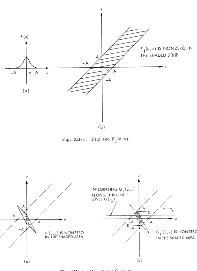
Let the Fourier transforms of f(t) and

h(t,T)

be F(u), and H(u, v), respectively. Let

fI (x, y) = 6(x+y) f(y),

where 6 is the Dirac delta function. The Fourier transform of fl (x, y) is

F

1

(u, v) = F(-u+v).

Let

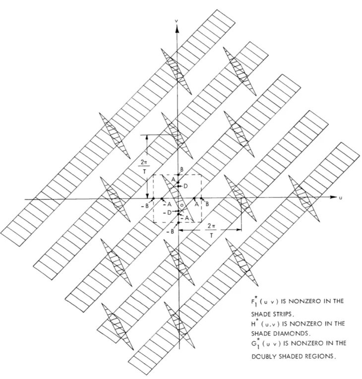
G

1(u, v) = F1

(u, v) H(u, v)

and

G(v)

G1(u, v) du.

Then the inverse Fourier transform of G(v) is g(t).

dB h(p, t-p) f(p).

(5)

F (u) -A oA u

(a)

Fig. XII-1.

v) IS NONZERO IN

;HADED STRIP

(b)

F(u) and F1(u, v).

INTEGRATING G₁(u,v) ALONG THIS LINE

GIVES G(vo)

- U

H (u,v) IS NONZERO IN THE SHADED AREA

Fig. XII-2.

-A

H(u, v) and G

1

(u, v).

(a)

V -V

O

G1 (u,v) IS NONZERO IN THE SHADED AREA

(6)

3. Graphical Interpretation

Assume that f(t) is bandlimited and has a bandwidth 2A, that is, F(u) = 0 for l u > A, as shown in Fig. XII-la. Then F_l(u, v) = F(-u+v) is zero outside an infinite strip bounded by the straight lines -u + v = ± A, as shown in Fig. XII- 1b. Now, if H(u, v) is zero outside the shaded region of Fig. XII-Za, then G_l(u, v) = Fl ( u , v) H(u, v) is zero outside the intersection of this region and the infinite strip, as shown in Fig. XII-2b. Integrating Gl(u, v) along the straight line v = vo gives G(v ) whose inverse Fourier transform is g(t). Therefore the bandwidth of g(t) is equal to the vertical extent of the

shaded region of Fig. XII-2b namely 2D.

4. Determination of Sampling Rate

Now, let us sample f(t) and h(t, T) with sampling periods T, and T X T, respectively,

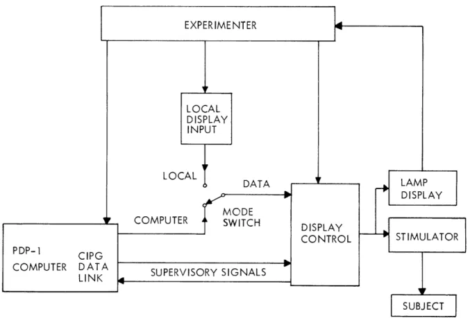
to get f (t) and h (t, T). _{The Fourier transforms of these latter functions, F (u), and} H (u, v), consist of periodically repeated versions of F(u) and H(u, v), respectively. Let

F₁(u, v) = F (-u+v) ₍₆₎

Gl(u, v) = F1(u, v) H (u, v) (7)

and

G (v) = G G_l(u, v) du. ₍₈₎

-00

Equation 7 is illustrated graphically in Fig. XII-3.

A sketch such as Fig. XII-3 is a convenient way of determining the sampling rate when we perform Eq. 1 on a digital computer. If we want the calculated values g (t) to be equal to the sampled values of g(t), and g(t) to be recoverable from g (t), then T should be chosen small enough so that Gl(u, v) consists of nonoverlapping

peri-odically repeated versions of Gl (u, v). Let the bandwidth of f(t) be 2A, and let the size of the smallest square which encloses the nonzero region of H(u, v) in the u-v plane be 2B X 2B. Then one might think that it is sufficient to choose T= , where C= Max(A, B). Not so. For example, if we let = _{2B in Fig. XII-3, then Gl(u, v) will contain} extra-neous components in addition to periodically repeated versions of G1 (u, v).

If we do not require that g *(t) be equal to the sampled values of g(t), but only require that g(t) be recoverable from g (t), then T should be chosen small enough so that G (v) = G(v), wherever G(v) is nonzero. This can be achieved by requiring that in the strip bounded by v = ±D in the u-v plane, G1 (u, v) consists of only nonoverlapping periodically repeated versions of Gl(u, v). For the example in Fig. XII-3, it is sufficient to

(7)

- B A a 1B -D -A 27T -B F1 (u v ) IS NONZERO IN THE SHADE STRIPS.

H (u,v) IS NONZERO IN THE SHADE DIAMONDS.

G1 ( u v ) IS NONZERO IN THE

DOUBLY SHADED REGIONS.

(8)

2IT

choose = A + B.

T

To require that g

(t)

be equal to the sampled values of g(t) obviously demands a

higher sampling rate than to require only that g(t) be recoverable from g (t). The former

is probably more convenient, however, since in the latter case, complicated

interpola-tion (lowpass filtering) may be needed to obtain sampled values of g(t) from g (t). In

the former approach, the sampling rate can be reduced, if we modify h(t,

T)

by setting

the value of H(u, v) to zero for all (u, v) not lying in the infinite strip determined by the

bandwidth of f(t).

T. S. Huang

References

1. T. Kailath, "Channel Characterization: Time-Variant Dispersive Channels," Chap. 6

in Lectures on Communication System Theory, E. J. Baghdady (ed.) (McGraw-Hill

Publishing Company, New York, 1961).

C. SURFACE RECONSTRUCTION FROM CONTOUR SAMPLES

The problem is the following: Given the constant elevation contours of some surface,

how should one reconstruct the surface.

If the surfaces of interest may be

character-ized statistically and, in particular, as a Gaussian random field, then the problem can

be approached.

Before going into the statistical approach there is another approach that is

actually reasonable.

The contours are treated as boundary conditions on which

the value of the surface is known.

From these boundary conditions, the

sur-face is

reconstructed by solving Laplace's equation.

This reconstruction

tech-nique is not really as arbitrary as it may seem, at first.

One of the most

useful properties of a contour map is that the height of the surface at any point

is bounded above and below by the heights of the neighboring contours unless

the neighboring contours have the same height.

A solution to Laplace's

equa-tion achieves its maximum and its minimum on the boundary, making the

solu-tion consistent with the property of a contour map.

A workable computer simulation of this idea is not yet successful.

One of

the biggest difficulties is in representing the contours on a grid.

A fine grid

requires too much computation, while a coarse grid may not be capable of

rep-resenting all of the contours.

One possibility is to use a fine grid where the

contours are dense and a coarse grid where the contours are sparse.

Suppose now that the surface is a sample function, x(t

1

,t

2

), from a Gaussian

random field.

The reconstruction problem may now be considered a statistical

estimation problem. If a minimum mean-square-error criterion is chosen, the

(9)

estimate will be the mean of the density of x(t

1

, t

2

) conditioned upon the contour

informa-tion. It is difficult to take into account all of the information in a contour map.

In

par-ticular, at any point

(s

l,

s

Z )

of the region where contour information is known, there is

an inequality: a(s

i

, s

)

<

x(s

1

, s

<

P(s1, s

).

This information is difficult to include in

the condition for the density so the condition will be simplified to apply

only to

the point

(tl' t

2

)

at which the estimate is desired.

Let the heights at which contours have been extracted be - = x

<

< ... < xn

oo.

Suppose that curves implicitly defined by x(t

1

,

tZ)= x

i,

i= 1,

... n-l

may be

param-eterized into the form (tli(u), t₂

i(u))

0 -< u < Ui. If (s' s2) is a point in the region ofl

interest, let

xj, x

k

(k=j

-

1,

j or j

+

1) be the heights of the contours "neighboring"' the

point (s'

s

). The boundary functions a(s

l ,

s2) and P(sl' s )

mentioned before may now

be defined.

min(xj, xk),

_if

_{x.j xk}

a(s_I, s2) = xj, _if_x(s 1, s2) > xj = xk

xj-1

_,

_if

_x(sl

,

SZ) <

x.

= x k

max(x , xk),

_if

_xj

_#

_xk

(s,

Sz) =

xj+

1

'

if x(sl, s

2

)

> x.

=

x k x , _if _x(s 1, s2) < x. = xk

These two functions are constant except for discontinuities on the contours.

The information contained in a contour map may now be written as the intersection

of two events: {x(tli(u), tzi(u)) = xi, for

0

-< u -< Ui, i = 1, ... , n-1} and

(a(s,

s ) -<

X(sl)

<

P(s1

,

s2)

}.

The two events in brackets are the conditions imposed on the

ran-dom process x(t

1, tZ ).

The first event

contains the information that would have been

obtained had the process been sampled on the contours; call this event S.

The second

event is information derived from the fact that all of the points are known at which the

surface achieves any of the heights x, ... xn-1.

If one knew the conditional density px(t

1

,

t

2 )

S(X

S)

and only the simplified version

of the second event,

C

= {a(t

l t

2)

x(t

l

P(t

'

tZ )},

were used,

then the mean

of

Px(tl, tz)S,

C would serve as the estimate of the field x(tl,

t).

The Gaussian

assumption for the random field enables one to find, conceptually, the density px(t

1

,t

2 )

S.

(10)

Px(tl,t 2) , C =

x(tl, t2) s(X S)

a(t)t2) Px(tl, t2) S ( U IS ) dU , (

X < a, X> p

To find px(tl' t2)I_{S ,}' one uses the fact that it must be a Gaussian density. The mean value function m(t 1, t2) must be a linear functional of values of x(t1, t2 ) along the con-tours and the variance -2 (tI, t2) may be found by knowing this linear functional. To simplify the notation, let t = (tl , t2) and let ti(u) = (tli(u), tZi(u)). The mean value function may be written as

n-1 m( t ) = h(t, ti(u)) x(ti(u)) du

i= 1

n-1 = x

.

h(t, ti(u)) du.

i= 1

Here the contours have been assumed to be parameterized by arc length u. The function h(t, ti(u)) must satisfy an integral equation:

n-1

R( t, t(v)) =

Ui h( t,

t

(u)) R( ti(u), t (v)) du,

i=l

where R(t, s) is the autocorrelation function of the random field. The variance may be written as

n-1

( ) = R(-, t) - I h(t, t.(u)) R(t, t.(u)) du. i= 1

The conditional density, px(T) S, C' may now be written as X~t) S, Cmynwbewitna

px()S, C(XIS, C)=

e

1 X - m

t()2

exp

(t )

1 X -m t

(t) exp - x M M dX

a(t) < X <

~(t)

(11)

and the estimate is the mean value of the density above:

exp(-

A

2

) -exp(-

B)

x(t)= m(t) +

W(t)

₂₁ 2

A0B

_exp(-.

)

_dz

A

a(t) - m(t)

P(t) - m(t)

where A = and B = . Because the density is restricted to [a(t),

P(t)],

the estimate must satisfy: a(t) < x (t) < p(t).

To simulate such an equation on the computer or to synthesize a device to realize

such an estimate would require the integral equation to be solved for each such contour

map. For this reason, a simpler approach is used by scanning the random field x(t

1

, t

2

)

to obtain a random process x(t).

The contours now become level-crossing times,

and the integral equation becomes a set of linear simultaneous equations. The equation

for the estimate remains essentially the same as before.

Assume that x(t) is to be estimated on a finite time interval, the level-crossing

times are t., j = 1,...,m and x(t )=1., where 1. is one of the x. levels.

Now

m

m (t) = a.(t)

1. j=1

and the a.(t) satisfy a set of linear simultaneous equations:

m

k

a

(t) p(tj, t

k )

=

p(t, tk),

k

=

1,..., m

j=1

and p(t, s) = E[x(t)x(s)].

The variance is

m

EZ(t)

_{= p (t, t) - I}

_{aj(t) p (t, tj).}

j=1

The estimate is the same as before, except now t replaces t.

The simplest version of this equation has been simulated; the mean value, m(t), and

variance,

-(t), are permitted to depend only upon the two neighboring crossing times.

The results of this simulation will be presented later.

G. M. Robbins

D. COMPUTER-CONTROLLED TACTILE DISPLAY

The display system described here is designed primarily as a research tool for

tac-tile experiments to determine the feasibility of word-at-a-time presentation of Braille

(12)

to the Blind. The system consists of the hardware and software necessary to simulta-neously present up to 8 Braille-like cells to a person's 8 fingers, one cell per finger.

1. System Hardware

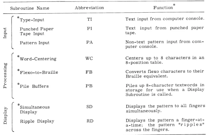
A block diagram of the display system is shown in Fig. XII-4. The system utilizes

Fig. XII-4. Diagram of the Display system.

the PDP-1 computer through the Cognitive Information Processing Group's data link. The local display input is a set of 18 switches that permit operation of the display inde-pendently from the computer. The mode switch selects whether data are to be received from the computer or from the local display input. The display control operates on these data to set up the corresponding patterns on the stimulator. In "computer" mode the display control also receives and sends back supervisory signals to the computer. The stimulator presents the information to the subject. The lamp display receives the same information as the stimulator, and serves as a monitor for the experimenter. The display is capable of presenting up to 48 bits simultaneously to the subject. The information is received 12 bits at a time from either the local display input or the

(13)

computer, and is stored in buffer registers in the display control before being gated to the stimulator. An individual Braille cell is presented to each finger by six solenoid-driven poke probes arranged in the 6-dot Braille cell configura-tion. Up to 8 characters may thus be presented simultaneously. Although the system uses, at present, this word-at-a-time Braille pattern of presentation, it

can easily accommodate a variety of stimulator patterns and devices.

2. System Software

The software of the system consists of a library of subroutines which can be used as building blocks to construct programs for specific tasks. The

sub-routines currently planned or available are summarized in Table XII-1. They are classified into Input, Processing, and Display subroutines. Input subroutines are used to read in data to the computer, either from punched paper tape or directly from the computer console. Processing subroutines convert the data to a standard format which is then used by one of the Display subroutines to pre-sent the necessary signals to the Display control to operate the stimulator.

Table XII-1. Summary of subroutines.

Subroutine Name Abbreviation Function

Type-Input TI Text input from computer console.

Punched Paper PI Text input from punched paper

Tape Input tape.

Pattern Input PA Non-text pattern input from

com-puter console.

Word-Centering WC Centers up to 8 characters in an

b4 8-position table.

-Flexo-to-Braille FB Converts flexo characters to their

a Braille equivalent.

o

Pile Buffers PB Piles up 8-character textwords in

storage for use when a Display Subroutine is called.

-

rSimultaneous

SD Displays the pattern to all fingers

Display simultaneously.

Ripple Display RD Displays the pattern a finger-at-a-time; the pattern "ripples"

across the fingers.

(14)

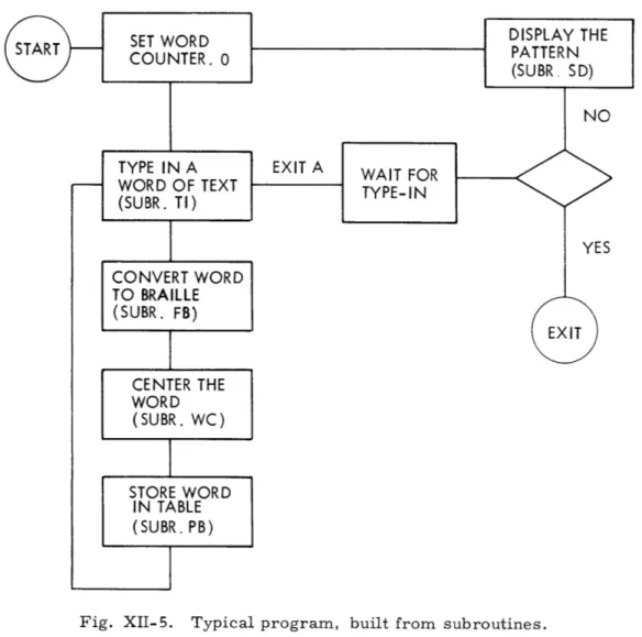
Fig. XII-5. Typical program, built from subroutines.

Other subroutines may easily be added to accommodate future experiments and applica-tions.

An example of a typical program is presented in Fig. XII-5. This program receives text typed into the computer console and displays it on the word-at-a-time Braille stim-ulator. After each word of text is typed in, it is converted to the Braille code, and centered with respect to the 8 fingers; the resulting centered Braille code is stored, and the next word of text can be typed in. After the desired text is completely typed in, typing a 'center dot' on the console followed by any other typed character (except '/')

causes the coded text to be displayed on the stimulator. Typing 'center dot' followed by '/' causes the program to exit.

An immediate application of the system would be as an output to a computerized reading machine for the Blind. By using a modified stimulator, the system could be applied to the study of tactual motion perception.

(15)

References

1. D. L. Peterson, "Computer-Controlled Tactile Display," S. M. Thesis, Department of Electrical Engineering, M. I. T., September 1967.

2. J. A. Williams, "Word-at-a-Time Tactile Display," S. M. Thesis, Department of Electrical Engineering, M. I. T., May 1966.

(16)