HAL Id: hal-02936452
https://hal.archives-ouvertes.fr/hal-02936452
Submitted on 11 Sep 2020
HAL is a multi-disciplinary open access
archive for the deposit and dissemination of sci-entific research documents, whether they are pub-lished or not. The documents may come from teaching and research institutions in France or abroad, or from public or private research centers.
L’archive ouverte pluridisciplinaire HAL, est destinée au dépôt et à la diffusion de documents scientifiques de niveau recherche, publiés ou non, émanant des établissements d’enseignement et de recherche français ou étrangers, des laboratoires publics ou privés.
Philippe Balbiani, Joseph Boudou, Martin Dieguez, David Fernández-Duque
To cite this version:
Philippe Balbiani, Joseph Boudou, Martin Dieguez, David Fernández-Duque. Bisimulations for in-tuitionistic temporal logics. Electronic Notes in Theoretical Computer Science, Elsevier, 2020. �hal-02936452�
Bisimulations for intuitionistic temporal logics
Philippe Balbiani
1,2Joseph Boudou
1,3IRIT, Toulouse University Toulouse, France
Mart´ın Di´
eguez
1,4IRIT, Toulouse University Toulouse, France University of Pau
Pau, France
David Fern´
andez-Duque
1,5IRIT, Toulouse University Toulouse, France
Department of Mathematics, Ghent University Ghent, Belgium
Abstract
We introduce bisimulations for the logic ITLewith ◯ (‘next’), U (‘until’) and R (‘release’), an intuitionistic temporal logic based on structures (W, ≼, S), where ≼ is used to interpret intuitionistic implication and S is a ≼-monotone function used to interpret the temporal modalities. Our main results are that ◇ (‘eventually’), which is definable in terms of U , cannot be defined in terms of ◯ and ◻, and similarly that ◻ (‘henceforth’), definable in terms of R, cannot be defined in terms of ◯ and U , even over the smaller class of here-and-there models.
Keywords: linear temporal logic, bisimulation, expressivity
1
Introduction
The definition and study of full combinations of modal [5] and intuitionistic [6,23] logics can be quite challenging [30], and temporal logics, such as LTL [28], are no exception. Some intuitionistic analogues of temporal logics have been proposed,
1 This research was partially supported by ANR-11-LABX-0040-CIMI within the program ANR-11-IDEX-0002-02. 2 Email: [email protected] 3 Email: [email protected] 4 Email: [email protected] 5 Email: [email protected]
This paper is electronically published in Electronic Notes in Theoretical Computer Science
including logics with ‘past’ and ‘future’ tenses [9], or with ‘next’ [7,19] and ‘hence-forth’ [17]. We proposed an alternative formulation in [4], where we defined the logics ITLe and ITLp using semantics similar to those of expanding and persistent products of modal logics, respectively [13], and the tenses ◯ (‘next’), ◇ (‘even-tually’), and ◻ (‘henceforth’). ITLe in particular differs from previous proposals (e.g. [9,27]) in that we consider minimal frame conditions that allow for all for-mulas to be upward-closed under the intuitionistic preorder, which we denote ≼. We then showed that ITLe with ◯ (‘next’), ◇ (‘eventually’), and ◻ (‘henceforth’) is decidable, thus obtaining the first intuitionistic analogue of LTL which contains the three tenses, is conservative over propositional intuitionistic logic, is interpreted over unbounded time, and is known to be decidable.
Note that both ◇ and ◻ are taken as primitives, in contrast with the classical case, where ◇ϕ may be defined by ◇ϕ ≡ ¬◻¬ϕ, whereas the latter equivalence is not intuitionistically valid. The same situation holds in the more expressive language with U (‘until’): while the language with ◯ and U is equally expressive to classical monadic first-order logic with ≤ over N [12], U admits a first-order definable intuitionistic dual, R (‘release’), which cannot be defined in terms of U using the classical definition. However, this is not enough to conclude that R cannot be defined in a different way. Thus, while in [4] we explored the question of decidability, here we will focus on definability; which of the modal operators can be defined in terms of the others?
Following Simpson [30] and other authors, we interpret the language of ITLe using bi-relational structures, with a partial order ≼ to interpret intuitionistic im-plication, and a function or relation, which we denote S, representing the passage of time. Alternatively, one may consider topological interpretations [8], but we will not discuss those here. Various intuitionistic temporal logics have been consid-ered, using variants of these semantics and different formal languages. The main contributions include:
● Davies’ intuitionistic temporal logic with ◯ [7] was provided Kripke semantics
and a complete deductive system by Kojima and Igarashi [19].
● Logics with ◯, ◻ were axiomatized by Kamide and Wansing [17], where ◻ was
interpreted over bounded time.
● Nishimura [25] provided a sound and complete axiomatization for an
intuition-istic variant of the propositional dynamic logic PDL.
● Balbiani and Di´eguez axiomatized the here-and-there variant of LTL with
◯, ◇, ◻ [2], here denoted ITLht.
● Fern´andez-Duque [10] proved the decidability of a logic based on topological
semantics with ◯, ◇ and a universal modality.
● The authors [4] proved that the logic ITLe with ◯, ◇, ◻ has the strong finite
model property and hence is decidable, yet the logic ITLp, based on a more restrictive class of frames, does not enjoy the fmp.
In this paper, we extend ITLe to include U (‘until’) and R (‘release’). As is well-known, ◇ϕ ≡ ⊺ U ϕ and ◻ϕ ≡ R ϕ; these equivalences remain valid in the intuitionistic setting, but many of the tenses are no longer inter-definable as in the classical case. To show this, we will introduce different notions of bisimulation which
preserve formulas with ◯ and each of ◇, ◻, U and R. With this, we will show that R (or even ◻) may not be defined in terms of U over the class of here-and-there models, while ◇ can be defined in terms of ◻, and U can be defined in terms of R over this class. However, we show that over the wider class of expanding models, ◇cannot be defined in terms of ◻.
2
Syntax and semantics
We will work in sublanguages of the language L given by the following grammar:
ϕ, ψ ∶= p ∣ ∣ ϕ ∧ ψ ∣ ϕ ∨ ψ ∣ ϕ → ψ ∣ ◯ ϕ ∣ ◇ϕ ∣ ◻ϕ ∣ ϕ U ψ ∣ ϕ R ψ
where p is an element of a countable set of propositional variables P. All sublan-guages we will consider include all Boolean operators and ◯, hence we denote them by displaying the additional connectives as a subscript; for example, L◇◻ denotes
the U -free, R-free fragment. As an exception to this general convention, L◯denotes
the fragment without ◇, ◻, U or R. As in the propositional case, ¬ϕdef= ϕ → . Given any formula ϕ, we define the length of ϕ (in symbols, ∣ϕ∣) recursively as follows:
● ∣p∣ = ∣∣ = 0;
● ∣φ ⊙ ψ∣ = 1 + ∣φ∣ + ∣ψ∣, with ⊙ ∈ {∨, ∧, →, R, U };
● ∣⊙ψ∣ = 1 + ∣ψ∣, with ⊙ ∈ {¬, ◯, ◻, ◇}.
Broadly speaking, the length of a formula ϕ corresponds to the number of connec-tives appearing in ϕ.
2.1 Dynamic posets
Formulas of L are interpreted over dynamic posets. A dynamic poset is a tuple D = (W, ≼, S), where W is a non-empty set of states, ≼ is a partial order, and S is a function from W to W satisfying the forward confluence condition that for all w, v ∈ W, if w ≼ v then S(w) ≼ S(v). An intuitionistic dynamic model, or simply model, is a tuple M = (W, ≼, S, V ) consisting of a dynamic poset equipped with a valuation function V from W to sets of propositional variables that is ≼-monotone, in the sense that for all w, v ∈ W, if w ≼ v then V (w) ⊆ V (v). In the standard way, we define S0(w) = w and, for all k > 0, Sk(w) = S (Sk−1(w)). Then we define the satisfaction relation ⊧ inductively by:
(i) M, w ⊧ p iff p ∈ V (w); (ii) M, w ⊭ ;
(iii) M, w ⊧ ϕ ∧ ψ iff M, w ⊧ ϕ and M, w ⊧ ψ; (iv) M, w ⊧ ϕ ∨ ψ iff M, w ⊧ ϕ or M, w ⊧ ψ; (v) M, w ⊧ ◯ϕ iff M, S(w) ⊧ ϕ; (vi) M, w ⊧ ϕ → ψ iff ∀v ≽ w, if M, v ⊧ ϕ, then M, v ⊧ ψ;
(vii) M, w ⊧ ◇ϕ iff there exists k s.t. M, Sk(w) ⊧ ϕ;
(viii) M, w ⊧ ◻ϕ iff for all k, M, Sk(w) ⊧ ϕ;
(ix) M, w ⊧ ϕ U ψ iff there exists k ≥ 0 s.t. M, Sk(w) ⊧ ψ and ∀i ∈ [0, k), M, Si(w) ⊧ ϕ;
(x) M, w ⊧ ϕ R ψ iff for all k ≥ 0, ei-ther M, Sk(w) ⊧ ψ, or ∃i ∈ [0, k) s.t. M, Si(w) ⊧ ϕ.
As usual, a formula ϕ is satisfiable over a class of models Ω if there is a model M ∈Ω and a world w of M so that M, w ⊧ ϕ, and valid over Ω if, for every world w of every model M ∈ Ω, M, w ⊧ ϕ. Satisfiability (validity) over the class of models based on an arbitrary dynamic poset will be called satisfiability (validity) for ITLe, or expanding domain linear temporal logic.6
The relation between dynamic posets and expanding products of modal logics is detailed in [4], where the following is also shown. Below, we use the notation JϕK= {w ∈ W ∣ M, w ⊧ ϕ}.
Lemma 2.1 Let D = (W, ≼, S), where (W, ≼) is a poset and S∶ W → W is any function. Then, D is a dynamic poset if and only if, for every valuation V on W and every formula ϕ,JϕK is ≼-monotone, i.e., if w ∈JϕK and v≽w, then v ∈JϕK.
Proof. The left to right direction is proved by induction on ϕ. The case of ϕ ∈ P is proved by using the condition on V . The rest of the inductive steps are routine. For instance, let us consider the case of ϕ U ψ and suppose that v ≽ w and w ∈ Jϕ U ψK. Then, there exists k ≥ 0 such that M, S
k(w) ⊧ ψ and for all 0 ≤ j < k,
M, Sj(w) ⊧ ϕ. Since S is confluent, an easy induction shows that Si(v) ≽ Si(w) for all 0 ≤ i ≤ k. Therefore, by induction hypothesis, we get M, Sk(v) ⊧ ψ and for all 0 ≤ j < k, M, Sj(v) ⊧ ϕ, hence v ∈
Jϕ U ψK. For the converse direction we assume that D = (W, ≼, S) and w, v ∈ W such that v ≽ w and S(w) /≼ S(v). Take p ∈ P and define V (u) = {p} if S(w) ≼ u, V (u) = ∅ otherwise. It is easy to see that V is ≼-monotone, but p /∈ V (S(v)) (because S(w) /≼S(v)) and p ∈ V (S(w)) (because S(w) ≼ S(w)), from which it follows that (D, V ), w ⊧ ◯p but (D, V ), v ⊭ ◯p. ◻
This suggests that dynamic posets provide suitable semantics for intuitionistic LTL. Moreover, dynamic posets are convenient from a technical point of view:
Theorem 2.2 ([4]) There exists a computable function B such that any formula ϕ ∈ L◇◻ satisfiable (resp. falsifiable) on an arbitrary model is satisfiable (resp.
fal-sifiable) on a model whose size is bounded by B(∣ϕ∣).
It follows that the L◇◻-fragment of ITL
e is decidable. Moreover, as we will
see below, many of the familiar axioms of classical LTL are valid over the class of dynamic posets, making them a natural choice of semantics for intuitionistic LTL.
2.2 Persistent posets
Despite the advantages of dynamic posets, in the literature one typically considers a more restrictive class of frames, as we define them below.
Definition 2.3 Let (W, ≼) be a poset. If S∶ W → W is such that, whenever v ≽ S(w), there is u ≽ w such that v = S(u), we say that S is backward confluent. If S is both forward and backward confluent, we say that it is persistent. A tuple (W, ≼, S) where S is persistent is a persistent intuitionistic temporal frame, and the set of valid formulas over the class of persistent intuitionistic temporal frames is denoted ITLp, or persistent domain LTL.
As we will see, persistent frames do have some technical advantages over arbi-trary dynamic posets. Nevertheless, they have a crucial disadvantage:
Theorem 2.4 ([4]) The logic ITLp does not have the finite model property, even for formulas in L◇◻.
2.3 Temporal here-and-there models
An even smaller class of models which, nevertheless, has many applications is that of temporal here-and-there models [2]. Some of the results we will present here apply to this class, so it will be instructive to review it. Recall that the logic of here-and-there is the maximal logic strictly between classical and intuitionistic propositional logic, given by a frame {0, 1} with 0 ≼ 1. The logic of here-and-there is obtained by adding to intuitionistic propositional logic the axiom p ∨ (p → q) ∨ ¬q.
A temporal here-and-there frame is a persistent frame that is ‘locally’ based on this frame. We can define here-and-there models using the following construction.
Definition 2.5 Let T be a set and f ∶ T → T . We define a dynamic poset HT(T, f ) = (W, ≼, S), with W = T × {0, 1}, (t, i) ≼ (s, j) if and only if t = s and i ≤ j, and S(t, i) = (f (t), i).
The prototypical example is the frame HT(N, f ), where f (n) = n + 1. Note, however, that our definition allows for other values of T (see Figure 1). In [2], this logic is axiomatized, and it is shown that ◻ cannot be defined in terms of ◇, a result we will strengthen here to show that ◻ cannot be defined even in terms of U . It is also claimed in [2] that ◇ is not definable in terms of ◻ over the class of here-and-there models, but as we will see in Proposition6.3, this claim is incorrect.
3
Some valid and non-valid ITL
e-formulas
In this section we explore which axioms of classical LTL are still valid in our setting. We start by showing that the intuitionistic version of the interaction and induc-tion axioms used in [2] remain valid in our setting. However, not all Fisher-Servi axioms [11], which are valid in the here-and-there LTL of [2], are valid in ITLe. Proposition 3.1 The following formulas:
(i) ◯ ↔ (ii) ◯ (ϕ ∧ ψ) ↔ (◯ϕ ∧ ◯ψ); (iii) ◯ (ϕ ∨ ψ) ↔ (◯ϕ ∨ ◯ψ); (iv) ◯ (ϕ → ψ) → (◯ϕ → ◯ψ); (v) ◻ (ϕ → ψ) → (◻ϕ → ◻ψ); (vi) ◻ (ϕ → ψ) → (◇ϕ → ◇ψ); (vii) ◇ (ϕ ∨ ψ) → (◇ϕ ∨ ◇ψ); (viii) ◻ϕ ↔ ϕ ∧ ◯◻ϕ; (ix) ϕ ∨ ◯◇ϕ ↔ ◇ϕ; (x) ◻ (ϕ → ◯ϕ) → (ϕ → ◻ϕ) (xi) ◻ (◯ϕ → ϕ) → (◇ϕ → ϕ).
are ITLe-valid.
Proof. Let us consider (x) and (xi). For (x), let M = (W, ≼, S) be any ITLe model and w ∈ W be such that M, w ⊧ ◻ (ϕ → ◯ϕ). Let v ≽ w be arbitrary and assume that M, v ⊧ ϕ. Then, by induction on i we obtain that Si(w) ≼ Si(v) for all i;
since M, Si(w) ⊧ ϕ → ◯ϕ for all i, it follows that M, Si(v) ⊧ ϕ → ◯ϕ for all i as well. Hence an easy induction shows that M, Si(v) ⊧ ϕ for all i, which means that M, v ⊧ ◻ϕ. Since w was arbitrary, we conclude that the formula (x) is valid.
For (xi), let M be as above and w ∈ W be such that M, w ⊧ ◻ (◯ϕ → ϕ). Let v ≽ w be such that M, v ⊧ ◇ϕ, and let n be least so that M, Sn(v) ⊧ ϕ. If n > 0 then from ◯ϕ → ϕ we obtain M, Sn−1(v) ⊧ ϕ, contradicting the minimality of n. We conclude that n = 0, hence M, v ⊧ ϕ.
The proofs for the rest of formulas are standard. ◻
Some of the well-known Fisher Servi axioms [11] are only valid on the class of persistent frames.
Proposition 3.2 The formulas
(i) (◯ϕ → ◯ψ) → ◯ (ϕ → ψ), (ii) (◇ϕ → ◻ψ) → ◻ (ϕ → ψ)
are not ITLe-valid. However they are ITLp-valid.
Proof. Let {p, q} be a set of propositional variables and let us consider the ITLe model M = (W, ≼, S, V ) defined as: 1) W = {w, v, u}; 2) S(w) = v, S(v) = v and S(u) = u; 3) v ≼ u; 4) V (p) = {u}. Clearly, M, u /⊧p → q, so M, v /⊧ p → q. By definition, M, w /⊧ ◯ (p → q) and M, w /⊧ ◻ (p → q); however, it can easily be checked that M, w ⊧ ◯p → ◯q and M, w ⊧ ◇p → ◻q, so M, w /⊧ (◯p → ◯q) → ◯ (p → q) and M, w /⊧ (◇p → ◻q) → ◻ (p → q).
Let us check their validity over the class of persistent frames. For (i), let M = (W, ≼, S, V ) be an ITLp model and w a world of M such that M, w ⊧ ◯ϕ → ◯ψ. Suppose that v ≽ S(w) satisfies M, v ⊧ ϕ. By backward confluence, there exists u ≽ w such that v = S(u), so that M, u ⊧ ◯ϕ and thus M, u ⊧ ◯ψ. But this means that M, v ⊧ ψ, and since v ≽ S(w) was arbitrary, M, S(w) ⊧ ϕ → ψ, i.e. M, w ⊧ ◯(ϕ → ψ).
Similarly, for (ii) let us assume that M = (W, ≼, S, V ) is an ITLp model and w a world of M such that M, w ⊧ ◇ϕ → ◻ψ. Consider arbitrary k ∈ N, and suppose that v ≽ Sk(w) is such that M, v ⊧ ϕ. Then, it is readily checked that the composition of backward confluent functions is backward confluent, so that in particular Sk is backward confluent. This means that there is u ≽ w such that Sk(u) = v. But then, M, u ⊧ ◇ϕ, hence M, u ⊧ ◻ψ, and M, v ⊧ ψ. It follows that M, Sk(w) ⊧ ϕ → ψ,
and since k was arbitrary, M, w ⊧ ◻(ϕ → ψ). ◻
We make a special mention of the schema ◻ (◻ϕ → ψ) ∨ ◻ (◻ψ → ϕ), which char-acterises the class of weakly connected frames [14] in classical modal logic. We say that a frame (W, R, V ) is weakly connected iff it satisfies the following first-order property: for every x, y, z ∈ W , if x R y and x R z, then either y R z, y = z, or z R y. Proposition 3.3 The axiom schema ◻ (◻ϕ → ψ) ∨ ◻ (◻ψ → ϕ) is not ITLht-valid. Proof. Let us consider the set of propositional variables {p, q}, T = {0, 1}, f ∶ T → T be given by f (x) = 1, and let M = (W, ≼, S, V ) be the here-and-there model based on HT(T, f ) with V (p) = {(0, 1), (1, 1)} and V (q) = {(1, 0), (1, 1)}. The reader can check that M, (0, 0) /⊧ ◻p → q and M, (0, 1) /⊧ ◻q → p. Consequently, M, w /⊧
Finally, we show that ◇ϕ (resp. ◻ϕ) can be defined in terms of U (resp. R) and the LTL axioms involving U and R are also valid in our setting:
Proposition 3.4 The following formulas are ITLe-valid:
(i) ϕ U ψ ↔ ψ ∨ (ϕ ∧ ◯ (ϕ U ψ)); (ii) ϕ R ψ ↔ ψ ∧ (ϕ ∨ ◯ (ϕ R ψ)); (iii) ϕ U ψ → ◇ψ; (iv) ◻ψ → ϕ R ψ; (v) ◇ϕ ↔ ⊺ U ϕ; (vi) ◻ϕ ↔ R ϕ; (vii) ◯(ϕ U ψ) ↔ ◯ϕ U ◯ψ; (viii) ◯(ϕ R ψ) ↔ ◯ϕ R ◯ψ.
Proof. We consider some cases below. For (i), from left to right, let us assume that M, w ⊧ ϕ U ψ. Therefore there exists k ≥ 0 s.t. M, Sk(w) ⊧ ψ and for all j satisfying 0 ≤ j < k, M, Sj(w) ⊧ ϕ. If k = 0 then M, w ⊧ ψ while, if k > 0 it follows that M, w ⊧ ϕ and M, S(w) ⊧ ϕ U ψ. Therefore M, w ⊧ ψ ∨ (ϕ ∧ ◯(ϕ U ψ)). From right to left, if M, w ⊧ ψ then M, w ⊧ ϕ U ψ by definition. If M, w ⊧ ϕ ∧ ◯(ϕ U ψ) then M, w ⊧ ϕ and M, S(w) ⊧ ϕ U ψ so, due to the semantics, we conclude that M, w ⊧ ϕ U ψ. In any case, M, w ⊧ ϕ U ψ.
For (ii), we work by contrapositive. From right to left, let us assume that M, w /⊧ ϕ R ψ. Therefore there exists k ≥ 0 s.t. M, Sk(w) /⊧ ψ and for all j satisfying 0 ≤ j < k, M, Sj(w) /⊧ϕ. If k = 0 then M, w /⊧ψ while, if k > 0 it follows that M, w /⊧ϕ and M, S(w) /⊧ϕ R ψ. In any case, M, w /⊧ψ∧(ϕ ∨ ◯(ϕ R ψ)). From left to right, if M, w /⊧ψ then M, w /⊧ϕ R ψ by definition. If M, w /⊧ϕ ∨ ◯(ϕ R ψ) then M, w /⊧ϕ and M, S(w) /⊧ϕ U ψ so, due to the semantics of R, we conclude that M, w /⊧ϕ R ψ. In any case, M, w /⊧ϕ R ψ.
For (vii), from left to right, let us assume that M, w ⊧ ◯ (ϕ U ψ). Therefore there exists k ≥ 0 s.t. M, Sk+1(w) ⊧ ψ and for all j satisfying 0 ≤ j < k, M, Sj+1(w) ⊧ ϕ. It follows from M, Sk+1(w) ⊧ ψ that M, Sk(w) ⊧ ◯ψ, and from M, Sj+1(w) ⊧ ϕ that M, Sj(w) ⊧ ◯ϕ for all j < k. We conclude that M, w ⊧ ◯ϕ U ◯ψ. Conversely, if M, w ⊧ ◯ϕ U ◯ψ, then there is k ≥ 0 so that M, Sk(w) ⊧ ◯ψ and, for all i < k, M, Si(w) ⊧ ◯ϕ. It follows that M, Sk+1(w) ⊧ ψ and, for all i < k, M, Si+1(w) ⊧ ϕ, witnessing that M, S(w) ⊧ ϕ U ψ and M, w ⊧ ◯(ϕ U ψ).
For (viii), we proceed similarly, but work by contrapositive. From right to left, let us assume that M, w /⊧ ◯ (ϕ R ψ). Therefore there exists k ≥ 0 s.t. M, Sk+1(w) /⊧ψ and for all j satisfying 0 ≤ j < k, M, Sj+1(w) /⊧ϕ. This implies that M, Sk(w) /⊧ ◯ψ and for all j satisfying 0 ≤ j < k, M, Sj(w) /⊧ ◯ϕ, hence M, w /⊧ ◯(ϕ R ψ). Similarly, if M, w /⊧ ◯(ϕ R ψ) then any k ≥ 0 so that M, Sk(w) /⊧ ◯ψ and, for all i < k, M, Si(w) /⊧ ◯ϕ yields M, Sk+1(w) /⊧ψ and, for all i < k, M, Si+1(w) /⊧ϕ, witnessing that M, S(w) /⊧ϕ R ψ and M, w /⊧ ◯(ϕ R ψ).
The proof of the remaining items is routine. ◻
As in the classical case, over the class of persistent models we can ‘push down’ all occurrences of ◯ to the propositional level. Say that a formula ϕ is in ◯-normal form if all occurrences of ◯ are of the form ◯ip, with p a propositional variable. Theorem 3.5 Given ϕ ∈ L, there exists ̃ϕ in ◯-normal form such that ϕ ↔ ̃ϕ is valid over the class of persistent models.
Proof. The claim can be proven by structural induction using the validities in
We remark that the only reason that this argument does not apply to arbi-trary ITLe models is the fact that (◯ϕ → ◯ψ) → ◯(ϕ → ψ) is not valid in general (Proposition3.2).
4
Bounded bisimulations for
◇ and ◻
In this section we adapt the classical definition of bounded bisimulations for modal logic [3] to our case. To do so we combine the ordinary definition of bounded bisimulations with the work of [26] on bisimulations for propositional intuitionistic logic. Such work introduces extra conditions involving the partial order ≼. In our setting, we combine both approaches in order to define bisimulation for a language involving ◇, ◻ and ◯ as modal operators plus an intuitionistic →. Since all languages we consider contain Booleans and ◯, it is convenient to begin with a ‘basic’ notion of bisimulation for this language.
Definition 4.1 Given n > 0 and two ITLe models M1 and M2, a sequence of
binary relations Zn⊆ ⋯ ⊆Z0⊆W1×W2 is said to be a bounded ◯-bisimulation if for all (w1, w2) ∈W1×W2 and for all 0 ≤ i < n, the following conditions are satisfied:
Atoms. If w1Ziw2then for all propositional variables p, M1, w1 ⊧p iff M2, w2 ⊧p. Forth →. If w1 Zi+1w2 then for all v1 ∈W1, if v1 ≽w1, there exists v2 ∈W2 such that v2≽w2 and v1Ziv2.
Back→. If w1Zi+1w2 then for all v2∈W2 if v2≽w2 then there exists v1∈W1 such that v1≽w1 and v1Ziv2.
Forth◯. if w1Zi+1w2 then S(w1) ZiS(w2).
Note that there is not ‘back’ clause for ◯; this is simply because S is a function, so its ‘forth’ and ‘back’ clauses are identical. Bounded ◯-bisimulations are useful because they preserve the truth of relatively small L◯-formulas.
Lemma 4.2 Given two ITLe models M1 and M2 and a bounded ◯-bisimulation
Zn⊆ ⋯ ⊆Z0 between them, for all 0 ≤ i ≤ n and (w1, w2) ∈W1×W2, if w1 Zi w2 then for all ϕ ∈ L◯ satisfying ∣ϕ∣ ≤ i
7, M
1, w1⊧ϕ iff M2, w2⊧ϕ.
Proof. We proceed by induction on i. Let 0 ≤ i ≤ n be such that for all j < i the lemma holds. Let w1 ∈W1 and w2 ∈W2 be such that w1 Ziw2 and let us consider ϕ ∈ L◇ such that ∣ϕ∣ ≤ i. The cases where ϕ is an atom or of the forms θ ∧ ψ, θ ∨ ψ
are as in the classical case and we omit them. Thus we focus on the following: Caseϕ = θ → ψ. We proceed by contrapositive to prove the left-to-right implication. Note that in this case we must have i > 0.
Assume that M2, w2⊧/θ → ψ. Therefore there exists v2∈W2 such that v2≽w2, M2, v2 ⊧θ, and M2, v2 ⊧/ ψ. By the Back →condition, it follows that there exists v1 ∈ W1 such that v1 ≽ w1 and v1 Zi−1 v2. Since ∣θ∣ ≤ i − 1 and ∣ψ∣ ≤ i − 1, by the induction hypothesis, it follows that M1, v1 ⊧ θ and M1, v1 ⊧/ ψ. Consequently,
7 Although not optimal, we use the length of the formula in this lemma for the sake of simplicity. More precise measures like counting the number of modalities and implications could be equally used.
M1, w1⊧/θ → ψ. The converse direction is proved in a similar way but usingForth →.
Case ϕ = ◯ψ. Once again we have that i > 0. Assume that M1, w1 ⊧ ◯ψ, so that
M1, S(w1) ⊧ψ. By Forth ◯, S1(w1) Zi−1 S2(w2). Moreover, ∣ψ∣ ≤ i − 1, so that by the induction hypothesis, M2, S(w2) ⊧ ψ, and M2, w2 ⊧ ◯ψ. The right-to-left
direction is analogous. ◻
Next, we will extend the notion of a bounded ◯-bisimulation to include other tenses. Let us begin with ◇.
Definition 4.3 Given n > 0 and two ITLe models M1 and M2, a bounded
◯-bisimulation Zn⊆ ⋯ ⊆Z0⊆W1×W2 is said to be a bounded ◇-bisimulation if for all (w1, w2) ∈W1×W2 and for all 0 ≤ i < n, if w1Zi+1w2, then the following conditions are satisfied:
Forth ◇. For all k1 ≥ 0 there exist k2 ≥ 0 and (v1, v2) ∈ W1 ×W2 such that Sk2(w2) ≽v2, v1≽Sk1(w1) and v1Ziv2.
Back◇. For all k2≥0 there exist k1≥0 and (v1, v2) ∈W1×W2 such that Sk1(w1) ≽ v1, v2≽Sk2(w2) and v1Ziv2.
The reader will notice that the clauses for ◇ involve the intuitionistic partial order, even though this is not involved in the semantics of ◇. However, this will give us more flexibility in designing bisimulations. The reason it works is that if k1
is so that Sk1(w1)witnesses that ◇ϕ is true on w1, then ϕ will also be true on any v1≽Sk1(w1) by the monotonicity of intuitionistic truth. Similarly, if Sk2(w2) ≽v2
and ϕ holds on v2, then it will also hold on Sk2(w2). Thus we do not need Sk1(w1) and Sk2(w2)to be directly connected by the bisimulation; rather, it is sufficient for v1, w1to act as ‘proxies’. As was the case of Lemma4.2, if two worlds are related by
a bounded ◇-bisimulation, then they satisfy the same L◇-formulas of small length.
Lemma 4.4 Given two ITLe models M1 and M2 and a bounded ◇-bisimulation
Zi⊆ ⋯ ⊆Z0 between them, for all 0 ≤ i ≤ n and (w1, w2) ∈W1×W2, if w1 Zi w2, then for all8 ϕ ∈ L◇ satisfying ∣ϕ∣ ≤ i, M1, w1⊧ϕ iff M2, w2⊧ϕ.
Proof. We proceed by induction on n. Let 0 ≤ i ≤ n be such that for all j < i the lemma holds. Let w1 ∈W1 and w2 ∈W2 be such that w1 Ziw2 and let us consider ϕ ∈ L◇ such that ∣ϕ∣ ≤ i. We only consider the case where ϕ = ◇ψ, as other cases
are covered by Lemma4.2.
From left to right, if M1, w1 ⊧ ◇ψ then there exists k1 ≥ 0 such that M1, Sk1(w1) ⊧ψ. ByForth◇, there exists k2≥0 and (v1, v2) ∈W1×W2 such that Sk2(w2) ≽v2, v1 ≽Sk1(w1) and v1Zi−1 v2. By ≼-monotonicity, M1, v1 ⊧ψ. Then, by the induction hypothesis and the fact that ∣ψ∣ ≤ i − 1, it follows that M2, v2 ⊧ψ, thus by ≼-monotonicity once again, M2, Sk2(w2) ⊧ ψ, so that M2, w2 ⊧ ◇ψ. The
converse direction is proved similarly by usingBack ◇. ◻
We can define bounded ◻-bisimulations in a similar way.
8 We remind the reader that, as per our convention, L◇is the ◻, U , R-free fragment. A similar comment applies to other sublanguages of L mentioned below.
Definition 4.5 A bounded ◯-bisimulation Zn⊆ ⋯ ⊆Z0⊆ W1 ×W2 is said to be a bounded ◻-bisimulation if for all (w1, w2) ∈ W1 ×W2 and for all 0 ≤ i < n, if
w1 Zi+1w2, then:
Forth◻. For all k2≥0 there exist k1≥0 and (v1, v2) ∈W1×W2 s.t. Sk2(w2) ≽v2, v1≽Sk1(w1) and v1Ziv2.
Back◻. For all k1 ≥0 there exist k2 ≥0 and (v1, v2) ∈W1×W2 s.t. Sk1(w1) ≽v1, v2≽Sk2(w2) and v1Ziv2.
The intuition for the role of v1, v2 in the clauses for ◻ is similar to that of ◇,
except that now we have to transfer negative information. If ◻ϕ fails at w1, there
will be k1 ≥ 0 so that ϕ fails on Sk1(w1); but then, ϕ will forcibly fail on any v1 ≼Sk1(w1). Similarly, if ϕ fails on v2 ≽Sk2(w2), ϕ will fail on Sk2(w2) as well, witnessing that ◻ϕ fails on w2.
Lemma 4.6 Given two ITLe models M1 and M2 and a bounded ◻-bisimulation
Zn⊆ ⋯ ⊆Z0 between them, for all (w1, w2) ∈W1×W2 and 0 ≤ i ≤ n, if w1 Zi w2 then for all ϕ ∈ L◻ such that ∣ϕ∣ ≤ i, then M1, w1⊧ϕ iff M2, w2⊧ϕ.
Proof. We proceed by induction on i. Let i ≥ 0 be such that for all j < i the lemma holds. Let w1 ∈W1 and w2∈W2 be such that w1 Ziw2 and let us consider ϕ ∈ L◻
such that ∣ϕ∣ ≤ i. Note that the cases for atoms as well as propositional and ◯ connectives are proved as in Lemma4.2, so we only consider ϕ = ◻ψ.
For the left-to-right implication, we work by contrapositive, and assume that M2, w2 ⊧ ◻/ ψ. Then, there exists k2≥0 such that M2, Sk2(w2) /⊧ψ. By Forth◻, there exist k1≥0 and (v1, v2) ∈W1×W2 s.t. Sk2(w2) ≽v2, v1≽Si1(w1)and v1 Zi−1 v2. As in the proof of Lemma4.4, by ≼-monotonicity, the induction hypothesis and
the fact that ∣ψ∣ ≤ i − 1, it follows that M1, v1⊧/ ψ; thus M1, Sk1(w1) /⊧ψ, and again by ≼-monotonicity M1, w1⊧ ◻ψ. The converse direction follows a similar reasoning/
but usingBack ◻. ◻
5
Bounded bisimulations for
U and R
In this section we adapt the bisimulations defined for a language with until and since [18] presented by Kurtonina and de Rijke [20] to our case. As with bisimula-tions for ◇ and ◻, we modify the standard clauses so that witnesses for U or R do not have to be directly connected, and, instead, it suffices for suitable ‘proxy’ worlds to be connected by the bisimulation. Let us begin with bounded bisimulations for U .
Definition 5.1 Given n ∈ N and two ITLe models M1 and M2, a bounded
◯-bisimulation Zn⊆ ⋯ ⊆Z0⊆W1×W2 is said to be a bounded U -bisimulation iff for all (w1, w2) ∈W1×W2, and for all 0 ≤ i < n if w1Zi+1w2 :
ForthU. For all k1≥0 there exist k2 ≥0 and (v1, v2) ∈W1×W2 such that (i) Sk2(w2) ≽v2, v1≽Sk1(w1) and v1Ziv2, and
(ii) for all j2 ∈ [0, k2) there exist j1 ∈ [0, k1) and (u1, u2) ∈ W1 ×W2 such that u1≽Sj1(w1), Sj2(w2) ≽u2 and u1Ziu2.
(i) Sk1(w1) ≽v1, v2≽Sk2(w2) and v1Ziv2, and
(ii) for all j1 ∈ [0, k1) there exist j2 ∈ [0, k2) and (u1, u2) ∈ W1 ×W2 such that
u2≽Sj2(w2), Sj1(w1) ≽u1 and u1Ziu2.
As was the case before, the following lemma states that two bounded U -bisimilar models agree on small LU formulas.
Lemma 5.2 Given two ITLe models M1 and M2 and a bounded U -bisimulation
Zn⊂ ⋯ ⊂Z0 between them, for all 0 ≤ m ≤ n and (w1, w2) ∈ W1×W2, if w1 Zm w2 then for all ϕ ∈ LU such that ∣ϕ∣ ≤ m, M1, w1⊧ϕ iff M2, w2⊧ϕ.
Proof. Once again, proceed by induction on n. Let m ≤ n be such that for all k < m the lemma holds. Let w1 ∈W1 and w2∈W2 be such that w1 Zmw2 and let us consider ϕ ∈ LU such that ∣ϕ∣ ≤ m. As before, we only consider the ‘new’ case, where
ϕ = θ U ψ. From left to right, assume that M1, w1⊧θ U ψ. Then, there exists i1≥0
such that M1, Si1(w1) ⊧ ψ and for all j1 satisfying 0 ≤ j1 < i1, M1, Sj1(w1) ⊧ θ. By Forth U , there exist i2 ≥0 and (v1, v2) ∈W1×W2 such that (i) Si2(w2) ≽ v2,
v1≽Si1(w1)and v1Zm−1v2; (ii) for all j2 satisfying 0 ≤ j2<i2 there exist j1∈ [0, i1) and (u1, u2) ∈W1×W2 s. t. u1≽Sj1(w1), Sj2(w2) ≽u2 and u1Zm−1u2.
From the first item, ≼-monotonicity, the fact that ∣ψ∣ ≤ m − 1, and the induction hypothesis, it follows that M2, Si2(w2) ⊧ψ. Take any j2 satisfying 0 ≤ j2<i2. By
the second item, the fact that ∣θ∣ ≤ m − 1, and the induction hypothesis, we conclude that M2, Sj2(w2) ⊧θ so M2, w2 ⊧θ U ψ. The right-to-left direction is symmetric
(but usingBackU ). ◻
Finally, we define bounded bisimulations for R.
Definition 5.3 A bounded ◯-bisimulation Zn⊆ ⋯ ⊆Z0⊆ W1 ×W2 is said to be a bounded R-bisimulation if for all (w1, w2) ∈ W1×W2 and for all 0 ≤ i < n, if w1 Zi+1w2 then :
ForthR. For all k2≥0 there exist k1 ≥0 and (v1, v2) ∈W1×W2 such that
(i) Sk2(w2) ≽v2, v1≽Sk1(w1) and v1Ziv2, and
(ii) for all j1 satisfying 0 ≤ j1<k1 there exist j2 such that 0 ≤ j2<k2 and (u1, u2) ∈
W1×W2 s. t. u1≽Sj1(w1), Sj2(w2) ≽u2 and u1Ziu2.
BackR. For all k1≥0 there exist k2≥0 and (v1, v2) ∈W1×W2 such that
(i) Sk1(w1) ≽v1, v2≽Sk2(w2) and v1Ziv2, and
(ii) for all j2 satisfying 0 ≤ j2<k2 there exist j1 such that 0 ≤ j1<k1 and (u1, u2) ∈
W1×W2 s. t. u2≽Sj2(w2), Sj1(w1) ≽u1 and u1Ziu2.
Once again, we obtain a corresponding bisimulation lemma for LR.
Lemma 5.4 Given two ITLe models M1 and M2 and a bounded R-bisimulation
Zn⊆ ⋯ ⊆Z0 between them, for all 0 ≤ m ≤ n and (w1, w2) ∈ W1×W2, if w1 Zm w2 then for all ϕ ∈ LU such that ∣ϕ∣ ≤ m, M1, w1⊧ϕ iff M2, w2⊧ϕ.
Proof. As before, we proceed by induction on n; the critical case where ϕ = θ R ψ follows by a combination of the reasoning for Lemmas4.6 and Lemma4.6. Details
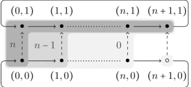
● (0, 0) ● (0, 1) n ● (1, 0) ● (1, 1) n − 1 ● (n, 0) ● (n, 1) 0 ○ (n + 1, 0) ● (n + 1, 1)
Fig. 1. The here-and-there model Hn. Black dots satisfy the atom p, white dots do not; all other atoms are false everywhere. Dashed lines indicate ≼ and solid lines indicate S. The ∼i-equivalence classes are shown as grey regions.
6
Definability and undefinability of modal operators
In this section, we explore the question of when it is that the basic connectives can or cannot be defined in terms of each other. It is known that, classically, ◇ and ◻ are interdefinable, as are U and R; we will see that this is not the case intuitionistically. On the other hand, U (and hence R) is not definable in terms of ◇, ◻ in the classical setting [18], and this result immediately carries over to the intuitionistic setting, as the class of classical LTL models can be seen as the subclass of that of dynamic posets where the partial order is the identity.
Interdefinability of modal operators can vary within intermediate logics. For example, ∧, ∨ and → are basic connectives in propositional intuitionistic logic, but in the intermediate logic of here-and-there [15], ∧ [1,2] and → [1] are basic operators while ∨ is definable in terms of → and ∧ [22]. In first-order here-and-there [21], the quantifier ∃ is definable in terms of ∀ and → [24] while ∀ is not definable in terms of the other operators. In the modal case, Simpson [30] shows that modal operators are not interdefinable in the logic IK and Balbiani and Di´eguez [2] proved the same result for the linear time temporal extension of here-and-there. This last proof is adapted to show that modal operators are not definable in ITLe. Note, however, that here we correct the claim of [2] stating that ◇ is not here-and-there definable in terms of ◻.
Let us begin by studying the definability of ◻ in terms of ◯ and U . Below, if L′ ⊆ L, ϕ ∈ L and Ω is a class of models, we say that ϕ is L′-definable over Ω if there is ϕ′
∈ L′ such that Ω ⊧ ϕ ↔ ϕ′.
Theorem 6.1 The connective ◻ is not LU-definable, even over the class of finite
here-and-there models.
Proof. Assume for the sake of contradiction that ◇p can be expressed as a U -free formula ϕ with ∣ϕ∣ = n > 0. Let T = {0, ⋯, n + 1} and f ∶ T → T be given by y = f (x) if and only if y ≡ x + 1 (mod n + 2). Then consider a here-and-there model Hn= (W, ≼, S, V ) based on HT(T, f ) and with V (p) = W ∖ {(n + 1, 0)}. For k ≤ n, define (i, j) ∼k(i′, j′) if (i, j) = (i′, j′)or
max{i(1 − j), i′
(1 − j′)} ≤n − k
(see Figure 1). Clearly, (Hn, (0, 0)) /⊧ ◇p, while (Hn, (0, 1)) ⊧ ◇p. Let us check
is increasing under inclusion. Moreover, ∼k is symmetric (indeed, an equivalence
relation) for eack k, so by symmetry, we only check theForthclauses.
Atoms: Assume that 0 ≤ k ≤ n and x ∼ky. Since (n + 1)(1 − 0) > n − k, either x = y
(so the two satisfy the same atoms) or x, y ≠ (n + 1, 0), so the two also satisfy the same atoms (namely, {p}).
Forth → : Let k satisfy 0 ≤ k < n and let us assume (i1, j1) ∼k+1 (i2, j2) and (i1, j1) ≼ (i′1, j ′ 1). If (i1, j1) = (i2, j2), then (i′2, j ′ 2) def
= (i′1, j1′) witnesses that the clause holds, so we assume otherwise. Let us define (i′
2, j ′ 2)
def
= (i2, 1). Then, (i2, j2) ≼ (i′2, j2′)and max{i′1(1−j1′), i2′(1−j2′)} =max{i′1(1−j1′), 0} = i′1(1−j1′) ≤n−k, meaning that (i′ 1, j ′ 1) ∼k(i′2, j ′ 2), as required.
Forth ◯ : Let k satisfy 0 ≤ k < n and let us consider (i1, j1) ∼k+1 (i2, j2). If (i1, j1) = (i2, j2), then also S(i1, j1) =S(i2, j2), so we assume otherwise. We claim that for ` ∈ {1, 2}, f (i`)(1 − j`) ≤n − k. If j`=1 this is obvious, otherwise from the
definition of ∼k+1 we obtain i` < n − k so that f (i`) =i`+1 ≤ n − k. We conclude that max{(f (i1)(1 − j1), f (i2+1)(1 − j2)} ≤n − k, so that S(i1, j1) ∼kS(i2, j2), as
required.
Forth U : Let k satisfy 0 ≤ k < n, and let us suppose that (i1, j1) ∼k+1 (i2, j2).
Assume moreover that (i1, j1) ≠ (i2, j2), as the other case is easy to check. Fix k1≥0 and define (i′
1, j ′
1) =Sk1(i1, j1). Let us define k2 =0, v1 = (i1, 1), and v2 = (i2, j2),
so that Sk2(i2, j2) = (i2, j2). Since max{i1(1 − 1), i2(1 − j2)} =i2(1 − j2) <n − k, we have that v1 ∼k v2 and satisfy Condition i. Note also that the Condition ii holds vacuously because of [0, k2) = ∅.
Consequently, (∼m)m≤n is a a bounded U -bisimulation. By using Lemma 5.2 and the fact that (0, 0) ∼n (0, 1) we get that (0, 0) and (0, 1) satisfy the same U -free formulas ψ with ∣ψ∣ ≤ n. However, (Hn, (0, 0)) /⊧ ϕ and (Hn, (0, 1)) ⊧ ϕ: a
contradiction. ◻
As a consequence:
Corollary 6.2 The connective R is not definable in terms of ◯ and U , even over the class of persistent models.
Proof. If we could define q R p, then we could also define ◻p ≡ R p. ◻
Proposition 6.3 Over the class of here-and-there models, ◇ is L◻-definable. To
be precise, ◇p is equivalent to
ϕ = (◻(p → ◻(p ∨ ¬p)) ∧ ◻(◯◻(p ∨ ¬p) → p ∨ ¬p ∨ ◯◻¬p)) → (◻(p ∨ ¬p) ∧ ¬◻¬p).
Proof. Let M = (T × {0, 1}, ≼, S, V ) be a here-and-there model with S(t, i) = (f (t), i) (see Section 2.3). Before proving that ϕ is equivalent to ◇p, we give some intuition. Essentially, ϕ contemplates three different ways that ◇p could hold in (M, x), where x = (x1, x2). It may be that ◻(p ∨ ¬p) holds, in which case (M, x)
is p. In this case, ◇p holds iff ¬◻¬p holds, as in the standard classical seman-tics. If ◻(p ∨ ¬p) fails, then M does not behave classically; for some n, Sn(x) falsifies p ∨ ¬p. For ϕ to be true, we then need for either ◻(p → ◻(p ∨ ¬p)) or ◻(◯◻(p ∨ ¬p) → p ∨ ¬p ∨ ◯◻¬p)) to fail. The formula ◻(p → ◻(p ∨ ¬p)) will fail exactly when there is m such that Sm(x) satisfies p (hence x satisfies ◇p), and M does not behave classically after m; that is, there is n > m so that Sn(x) falsifies p ∨ ¬p. Meanwhile, ◻(◯◻(p ∨ ¬p) → p ∨ ¬p ∨ ◯◻¬p)) will fail exactly when there is m such that Sm(x) satisfies p but M behaves classically after m; in other words, Sn(x) falsifies p ∨ ¬p only for n < m. In this case, ◯◻(p ∨ ¬p) → p ∨ ¬p ∨ ◯◻¬p will be falsified exactly at the greatest such n.
Now for the proof. Assume that x = (x1, x2)is such that (M, x) ⊧ ◇p. To check that (M, x) ⊧ ϕ, let x′
≽ x, so that x′ = (x1, x2′) with x′2 ≥ x2, and consider the following cases.
Case(M, x′) ⊧ ◻(p ∨ ¬p). In this case, it is easy to see that we also have (M, x′) ⊧ ¬◻¬p given that (M, x) ⊧ ◇p.
Case (M, x′) /⊧ ◻(p ∨ ¬p). Using the assumption that (M, x) ⊧ ◇p, choose k such that (M, (fk(x1), x2)) ⊧p and consider two sub-cases.
(i) Suppose there is k′
>k such that (M, (fk
′
(x1), x′2)) /⊧p ∨ ¬p. Then, it follows that (M, (fk(x1), x′2)) /⊧p → ◻p ∨ ¬p and hence (M, x′) /⊧ ◻(p → ◻(p ∨ ¬p)). (ii) If there is not such k′, then there must be a maximal k′
< k such that (M, (fk′(x1), x′2)) ⊧/ p ∨ ¬p (otherwise, we would be in Case (M, x
′
) ⊧ ◻(p ∨ ¬p)). It is easily verified that
(M, (fk
′
(x1), x′2)) /⊧ ◯◻(p ∨ ¬p) → p ∨ ¬p ∨ ◯◻¬p,
and hence
(M, x′) /⊧ ◻(◯◻(p ∨ ¬p) → p ∨ ¬p ∨ ◯◻¬p).
Note that the above direction does not use any properties of here-and-there mod-els, and works over arbitrary expanding models. However, we need these properties for the other implication. Suppose that (M, x) ⊧ ϕ. If (M, x) ⊧ ◻(p ∨ ¬p) ∧ ¬◻¬p, then it is readily verified that (M, x) ⊧ ◇p. Otherwise,
(M, x) /⊧ ◻(p → ◻(p ∨ ¬p)) ∧ ◻(◯◻(p ∨ ¬p) → p ∨ ¬p ∨ ◯◻¬p).
If (M, x) /⊧ ◻(p → ◻(p ∨ ¬p)), then there is k such that
(M, (fk(x1), x2)) /⊧p → ◻(p ∨ ¬p).
This is only possible if x2 = 0 and (M, (fk(x1), x2)) ⊧ p, so that (M, x) ⊧ ◇p. Similarly, if
(M, x) /⊧ ◻(◯◻(p ∨ ¬p) → p ∨ ¬p ∨ ◯◻¬p),
then there is k such that (M, (fk(x1), x2)) /⊧ ◯◻(p∨¬p) → p∨¬p∨◯◻¬p. This is only possible if x2 =0, (M, (fk(x1), x2)) ⊧ ◯◻(p ∨ ¬p) and (M, (fk(x1), x2)) /⊧ ◯◻¬p. But from this it easily can be seen that there is k′
>k with (M, (fk
′
(x1), x2)) ⊧p,
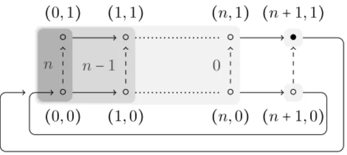
○ (0, 0) ○ (0, 1) n ○ (1, 0) ○ (1, 1) n − 1 ○ (n, 0) ○ (n, 1) 0 ○ (n + 1, 0) ● (n + 1, 1)
Fig. 2. The expanding model En. Notation is as in Figure1.
Corollary 6.4 Over the class of here-and-there models, p U q is LR-definable using
the equivalence p U q ≡ (q R(p ∨ q)) ∧ ◇q.
Hence, if we want to prove the undefinability of ◇ in terms of other operators, we must turn to a wider class of models, as we will do next.
Theorem 6.5 The operator ◇ cannot be defined in terms of ◻ over the class of finite expanding models.
Proof. Given n > 0, consider a model En = (W, ≼, S, V ) with W = {0, ⋯, n + 1} × {0, 1}, (i, j) ≼ (i′, j′
) if i = i′ and j ≤ j′, S(i, j) = (i + 1, j) if i ≤ n, S(n + 1, j) = (0, 0), and V (p) = {(n + 1, 1)}. For m ≤ n, define (i, j) ∼m (i′, j′) if either (i, j) = (i′, j′), or max{i, i′} ≤n − m. Then, it can easily be checked that (M, (0, 0)) /⊧ ◇p, (M, (0, 1)) ⊧ ◇p, and (0, 0) ∼m(0, 1).
It remains to check that (∼m)m≤n is a bounded ◻-bismulation. We focus on the ◻ clauses, and by symmetry, prove only Back ◻. Suppose that (i1, j1) ∼m (i2, j2) and fix k1 ≥ 0. Let (i′1, j1′) = Sk1(i1, j1). Choose k2 > n + 1 such that i2+k2 ≡ i′1 (mod n + 1), and let (i′2, j2′) = Sk2(i2, j2). It is not hard to check that i′1 =i′2 and j′
2 =0, from which we obtain (i ′ 2, j ′ 2) ≼ (i ′ 1, j ′
1). Hence, setting v1 =v2 = (i′2, j2′) gives us the desired witnesses.
By letting n vary, we see that no L◻-formula can be equivalent to ◇p. ◻
7
Conclusions
In this paper we have investigated on ITLe, an intuitionistic analogue of LTL based on expanding domain models from modal logic. We have shown that, as happens in other modal intuitionistic logics or modal intermediate logics, modal operators are not interdefinable.
Many open questions remain regarding intuitionistic temporal logics. We know that ITLeis decidable, but the proposed decision procedure is non-elementary. How-ever, there seems to be little reason to assume that this is optimal, raising the following question:
Question 1 Are the satisfiability and validity problems for ITLe elementary? Meanwhile, we saw in Theorems2.2and2.4that ITLehas the strong finite model property, while ITLpdoes not have the finite model property at all. However, it may yet be that ITLp is decidable despite this.
Question 2 Is ITLp decidable?
Regarding expressive completeness, it is known that LTL is expressively com-plete [18,29,12,16]; there exists a one-to-one correspondence (over N) between the temporal language and the monadic first-order logic equipped with a linear order and ‘next’ relation [12]. It is not known whether the same property holds between ITLe and first-order intuitionistic logic.
Question 3 Is L equally expressive to monadic first-order logic over the class of dynamic or persistent models?
Finally, a sound and complete axiomatization for ITLeremains to be found. The results we have presented here could be a first step in this direction, and we conclude with the following:
Question 4 Are the ITLe-valid formulas listed in this work, together with the intu-itionistic tautologies and standard inference rules, complete for the class of dynamic posets? Is the logic augmented with (◯p → ◯q) → ◯(p → q) complete for the class of persistent models?
References
[1] F. Aguado, P. Cabalar, D. Pearce, G. P´erez, and C. Vidal. A denotational semantics for equilibrium logic. TPLP, 15(4-5):620–634, 2015.
[2] P. Balbiani and M. Di´eguez. Temporal here and there. In M. Loizos and A. Kakas, editors, Logics in Artificial Intelligence, pages 81–96. Springer, 2016.
[3] P. Blackburn, M. de Rijke, and Y. Venema. Modal Logic. Cambridge University Press, New York, NY, USA, 2001.
[4] J. Boudou, M. Di´eguez, and D. Fern´andez-Duque. A decidable intuitionistic temporal logic, 2017. [5] A.V. Chagrov and M. Zakharyaschev. Modal Logic, volume 35 of Oxford logic guides. Oxford University
Press, 1997.
[6] D. Van Dalen. Intuitionistic logic. In Handbook of Philosophical Logic, volume 166, pages 225–339. Springer Netherlands, 1986.
[7] R. Davies. A temporal-logic approach to binding-time analysis. In Proceedings, 11th Annual IEEE Symposium on Logic in Computer Science, New Brunswick, New Jersey, USA, July 27-30, 1996, pages 184–195, 1996.
[8] J.M. Davoren. On intuitionistic modal and tense logics and their classical companion logics: Topological semantics and bisimulations. Annals of Pure and Applied Logic, 161(3):349–367, 2009.
[9] W.B. Ewald. Intuitionistic tense and modal logic. The Journal of Symbolic Logic, 51(1):166–179, 1986. [10] D. Fern´andez-Duque. The intuitionistic temporal logic of dynamical systems. arXiv, 1611.06929
[math.LO], 2016.
[11] G Fischer Servi. Axiomatisations for some intuitionistic modal logics. In Rend. Sem. Mat. Univers. Polit. Torino, volume 42, pages 179–194, Torino, Italy, 1984.
[12] D. Gabbay, A. Pnueli, S. Shelah, and J. Stavi. On the Temporal Analysis of Fairness. In Proc. of the 7th ACM SIGPLAN-SIGACT Symposium on Principles of Programming Languages (POPL’80), pages 163–173, Las Vegas, Nevada, USA, 1980.
[13] D. Gabelaia, A. Kurucz, F. Wolter, and M. Zakharyaschev. Non-primitive recursive decidability of products of modal logics with expanding domains. Annals of Pure and Applied Logic, 142(1-3):245– 268, 2006.
[14] R. Goldblatt. Logics of Time and Computation. Number 7 in CSLI Lecture Notes. Center for the Study of Language and Information, Stanford, California, 2 edition, 1992. second edition.
[15] A. Heyting. Die formalen Regeln der intuitionistischen Logik. Sitzungsberichte der Preussischen Akademie der Wissenschaften. Physikalisch-mathematische Klasse. De¨utsche Akademie der Wissenschaften zu Berlin, Mathematisch-Naturwissenschaftliche Klasse, 1930.
[16] I Hodkinson. Expressive completeness of until and since over dedekind complete linear time. Modal logic and process algebra, 53:171–185, 1995.
[17] N. Kamide and H. Wansing. Combining linear-time temporal logic with constructiveness and paraconsistency. J. Applied Logic, 8(1):33–61, 2010.
[18] H. Kamp. Tense Logic and the Theory of Linear Order. PhD thesis, University of California, Los Angeles, California, USA, 1968.
[19] K. Kojima and A. Igarashi. Constructive linear-time temporal logic: Proof systems and Kripke semantics. Information and Computation, 209(12):1491 – 1503, 2011.
[20] N. Kurtonina and M. de Rijke. Bisimulations for temporal logic. Journal of Logic, Language and Information, 6(4):403–425, 1997.
[21] V. Lifschitz, D. Pearce, and A. Valverde. A Characterization of Strong Equivalence for Logic Programs with Variables, page 188–200. Springer Berlin Heidelberg, Berlin, Heidelberg, 2007.
[22] J. Lukasiewicz. Die logik und das grundlagenproblem. Les Entreties de Z¨urich sur les Fondaments et la M´ethode des Sciences Math´ematiques, 12(6-9):82–100, 1938.
[23] G. Mints. A Short Introduction to Intuitionistic Logic. 2000.
[24] Grigori Mints. Cut-free formulations for a quantified logic of here and there. Annals of Pure and Applied Logic, 162(3):237–242, 2010.
[25] H. Nishimura. Semantical analysis of constructive PDL. Publications of the Research Institute for Mathematical Sciences, Kyoto University, 18:427–438, 1982.
[26] A. Patterson. Bisimulation and propositional intuitionistic logic, page 347–360. Springer Berlin Heidelberg, Berlin, Heidelberg, 1997.
[27] G. Plotkin and C. Stirling. A framework for intuitionistic modal logics: Extended abstract. In Proceedings of the 1986 Conference on Theoretical Aspects of Reasoning About Knowledge, TARK ’86, pages 399–406, San Francisco, CA, USA, 1986. Morgan Kaufmann Publishers Inc.
[28] A. Pnueli. The temporal logic of programs. In Proceedings 18th IEEE Symposium on the Foundations of CS, pages 46–57, 1977.
[29] A. Rabinovich. A Proof of Kamp’s Theorem. Logical Methods in Computer Science, 10(1), 2014. [30] A.K. Simpson. The proof theory and semantics of intuitionistic modal logic. PhD thesis, University of