HAL Id: hal-00305069
https://hal.archives-ouvertes.fr/hal-00305069
Submitted on 3 May 2007
HAL is a multi-disciplinary open access
archive for the deposit and dissemination of
sci-entific research documents, whether they are
pub-lished or not. The documents may come from
teaching and research institutions in France or
abroad, or from public or private research centers.
L’archive ouverte pluridisciplinaire HAL, est
destinée au dépôt et à la diffusion de documents
scientifiques de niveau recherche, publiés ou non,
émanant des établissements d’enseignement et de
recherche français ou étrangers, des laboratoires
publics ou privés.
storage variations
R. Klees, E. A. Zapreeva, H. C. Winsemius, H. H. G. Savenije
To cite this version:
R. Klees, E. A. Zapreeva, H. C. Winsemius, H. H. G. Savenije. The bias in GRACE estimates of
continental water storage variations. Hydrology and Earth System Sciences Discussions, European
Geosciences Union, 2007, 11 (4), pp.1227-1241. �hal-00305069�
www.hydrol-earth-syst-sci.net/11/1227/2007/ © Author(s) 2007. This work is licensed under a Creative Commons License.
Earth System
Sciences
The bias in GRACE estimates of continental water storage
variations
R. Klees1, E. A. Zapreeva1, H. C. Winsemius2, and H. H. G. Savenije2
1Delft Institute of Earth Observation and Space Systems (DEOS), Delft University of Technology, The Netherlands 2Department of Water Management, Delft University of Technology, The Netherlands
Received: 11 October 2006 – Published in Hydrol. Earth Syst. Sci. Discuss.: 21 November 2006 Revised: 19 March 2007 – Accepted: 12 April 2007 – Published: 3 May 2007
Abstract. The estimation of terrestrial water storage
varia-tions at river basin scale is among the best documented ap-plications of the GRACE (Gravity and Climate Experiment) satellite gravity mission. In particular, it is expected that GRACE closes the water balance at river basin scale and al-lows the verification, improvement and modeling of the re-lated hydrological processes by combining GRACE ampli-tude estimates with hydrological models’ output and in-situ data.
When computing monthly mean storage variations from GRACE gravity field models, spatial filtering is mandatory to reduce GRACE errors, but at the same time yields biased amplitude estimates.
The objective of this paper is three-fold. Firstly, we want to compute and analyze amplitude and time behaviour of the bias in GRACE estimates of monthly mean water storage variations for several target areas in Southern Africa. In par-ticular, we want to know the relation between bias and the choice of the filter correlation length, the size of the target area, and the amplitude of mass variations inside and outside the target area. Secondly, we want to know to what extent the bias can be corrected for using a priori information about mass variations. Thirdly, we want to quantify errors in the estimated bias due to uncertainties in the a priori information about mass variations that are used to compute the bias.
The target areas are located in Southern Africa around the Zambezi river basin. The latest release of monthly GRACE gravity field models have been used for the period from Jan-uary 2003 until March 2006. An accurate and properly cal-ibrated regional hydrological model has been developed for this area and its surroundings and provides the necessary a priori information about mass variations inside and outside the target areas.
Correspondence to: R. Klees
The main conclusion of the study is that spatial smoothing significantly biases GRACE estimates of the amplitude of an-nual and monthly mean water storage variations and that bias correction using existing hydrological models significantly improves the quality of GRACE estimates. For most of the practical applications, the bias will be positive, which im-plies that GRACE underestimates the amplitudes. The bias is mainly determined by the filter correlation length; in the case of 1000 km smoothing, which is shown to be an appro-priate choice for the target areas, the annual bias attains val-ues up to 50% of the annual storage; the monthly bias is even larger with a maximum value of 75% of the monthly storage. A priori information about mass variations can provide rea-sonably accurate estimates of the bias, which significantly improves the quality of GRACE water storage amplitudes. For the target areas in Southern Africa, we show that after bias correction, GRACE annual amplitudes differ between 0 and 30 mm from the output of a regional hydrological model, which is between 0% and 25% of the storage. Annual phase shifts are small, not exceeding 0.25 months, i.e. 7.5 deg. It is shown that after bias correction, the fit between GRACE and a hydrological model is overoptimistic, if the same hydrolog-ical model is used to estimate the bias and to compare with GRACE. If another hydrological model is used to compute the bias, the fit is less, although the improvement is still very significant compared with uncorrected GRACE estimates of water storage variations. Therefore, the proposed approach for bias correction works for the target areas subject to this study. It may also be an option for other target areas pro-vided that some reasonable a priori information about water storage variations are available.
1 Introduction
The Gravity Recovery and Climate Experiment (GRACE), launched in March of 2002, has been designed to measure the Earth’s time variable gravity field at approximately monthly intervals with a spatial resolution of a few hundred kilome-ters. So far, 34 monthly gravity field solutions (April 2002– March 2006) have been released to the scientific community. Each solution consists of a set of spherical harmonic coef-ficients complete to degree and order 120. Differences be-tween two monthly solutions reflect temporal gravity varia-tions. They are caused by post glacial rebound, mass trans-port in the atmosphere and the oceans, and the redistribution of water, snow and ice on land. Prior to gravity field esti-mation, GRACE measurements have already been corrected for the major contribution of ocean and atmospheric mass variations. Therefore, differences between two monthly so-lutions mainly reflect changes in terrestrial water storage, i.e. groundwater, soil moisture, rivers, lakes, snow, and ice.
As a result, GRACE promises to provide new hydrological information in the form of estimates of monthly mean water storage variations over river basins having length scales of a few hundred kilometers and larger. This would allow the clo-sure of the water balance for river basins and the verification and improvement of the modelling of the related hydrolog-ical processes by combining GRACE estimates of monthly mean water storage variations with hydrological observations and hydrological model output.
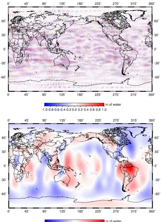
However, GRACE estimates of monthly mean water stor-age variations are erroneous due to measurement noise and the aliasing of unmodelled high-frequency mass variations into the monthly GRACE gravity field solutions (Swenson and Wahr, 2002; Wahr et al., 1998, 2006; Swenson and Wahr, 2006). Figure 1 shows the difference between two monthly gravity field solutions expressed in terms of equivalent wa-ter heights without smoothing and with 1000 km Gaussian smoothing.
The trackiness of the plot, which is typical for GRACE monthly solutions, is due to GRACE data errors and er-rors in the background models used in the pre-processing of GRACE data, and can be much larger than the mass varia-tion. To reduce these errors, spatial filtering (i.e. smoothing) is routinely applied. Unfortunately, spatial filtering biases the GRACE estimates of monthly mean mass variations. It is the subject of optimal filter design to find a filter that minimizes the sum of GRACE errors and filter errors.
The subject of this paper is to analyze the bias in GRACE estimates and to investigate to what extent the bias can be re-duced when using a priori information about mass variations. This improves the understanding of the potential and limita-tions of GRACE estimates of monthly mean water storage variations and is the basis for the design of an optimal filter for the target area at hand.
The paper is organized as follows: in Sect. 2, the relation between mass variations inside and outside the target area,
spatial smoothing, and bias has been established. In particu-lar, an alternative representation of the bias has been derived, which shows explicitly the contribution to the bias of mass variations inside and outside the target area. The approach to be followed in this study is outlined in Sect. 3. Informa-tion about mass variaInforma-tions inside and outside the target area is needed to compute the bias. We use the regional hydrolog-ical model LEW to provide this information for four target areas in Southern Africa centred at the upper Zambezi sub-catchment. The model is described in Sect. 4. The results of the analysis are presented in Sect. 5. This includes a time se-ries of the bias for the period January 2003 until March 2006 for each target area and various choices of spatial filtering, and a comparison of GRACE bias-corrected and uncorrected monthly mean water storage variations with the output of the LEW hydrological model. In particular, it has been shown that after bias correction, the agreement between LEW and GRACE are on the level of several millimeters, which gives an indication of residual errors in smoothed GRACE data and LEW model errors. Finally, uncertainties in the LEW model output have been estimated using Monte-Carlo simulations, and propagated into the bias. This gives an idea about the quality of a priori water storage variations needed to com-pute the bias.
Section 6 contains a summary of the results and the main conclusions of this study. In particular, some advice concern-ing the use of GRACE models and bias computation has been given.
2 GRACE monthly mean mass variations, spatial
filter-ing, and bias
Monthly GRACE gravity field models are very noisy (cf. Fig. 1). When computing the monthly mean water stor-age variation over a target area, the noise is partially reduced, but still unacceptable high. Therefore, some additional spa-tial smoothing is required prior to the computation of mean monthly mass variations over a target area. Isotropic Gaus-sian smoothing is widely used in many GRACE related stud-ies (e.g. Jekeli, 1981; Wahr et al., 1998). More advanced ap-proaches include non-isotropic smoothing kernels (e.g. Han et al., 2005) or Wiener filters, which use a priori information about noise and signal (i.e. water storage) (e.g. Swenson and Wahr, 2002).
Spatial smoothing reduces noise, but also introduces a bias in the estimated monthly mean water storage varia-tion. This bias leads to a significant amplitude reduction in estimated monthly mean water storage variations. There-fore, Velicogna and Wahr (2006) re-scaled the amplitude es-timates for Antarctica by a factor of 1.61; Fenoglio-Marc et al. (2006) applied a factor of 1.79 for the Mediterranean Sea; Chen et al. (2007) found a scaling factor of 1.33 for the Amazon and Mississippi basins and 1.54 for the Ganges and Zambezi basins.
Fig. 1. Global monthly mean water storage variation between April and March 2003 from GRACE. Top panel – without smoothing, Bottom
panel – after 1000 km Gaussian smoothing.
In appendix it is shown that the bias in the GRACE monthly mean water storage estimate can be written as ¯ε0= 1 4π R2 Z σ0 f0(χ − W ) dσR− 1 4π R2 Z σR−σ0 flW dσR, (1) where f0is the mass variation inside the target area, fl the mass variations outside the target area, χ the characteristic function of the target area, and W the target area filter func-tion, which is the spherical convolution of the spatial filter
function (e.g. the Gaussian kernel) with the characteristic function χ . σ0 is the target area and σR is the mean Earth sphere. According to Eq. (1), the bias consists of two terms. The first term on the right-hand side of Eq. (1) is called type 1
error. It expresses the contribution of mass variations inside
the target area to the bias. Since χ −W is always positive, it causes an underestimation of the amplitude of the monthly mean mass variation averaged over the target area. The sec-ond term on the right-hand side of Eq. (1) is called type 2
error. It represents the contribution of mass variations
out-side the target area to the bias. If the mass variations inout-side and outside the target area are “in phase” (i.e. they have the same sign), the sum of the two terms of the right-hand side of Eq. (1) is always smaller than each individual term; in other words, the two bias contributors cancel to some extent. That may be the reason why in literature (e.g. Chen et al., 2005a,b)
filtered GRACE solutions fit quite well with unfiltered
esti-mates of the monthly mean storage variation from hydrolog-ical models. The sum of the two error terms will attain a maximum if there are no mass variations outside the target area or, even more extreme, if the mass variation outside the target area differs in sign from the mass variation inside the target area. Note that ¯ε0 is sometimes called leakage error (e.g. Wahr et al., 1998; Swenson and Wahr, 2002; Swenson et al., 2003); sometimes the term leakage error only refers to the type 2 error (e.g. Klees et al., 2006).
3 Approach
In this study, we want to analyse the time behaviour of the bias, due to spatial smoothing in GRACE monthly mean water storage variations for various target areas in Southern Africa; moreover we want to investigate how accurately the bias can be estimated using a priori information about the mass variations. The following approach is followed:
– To quantify the bias, we need information about the
mass variation inside (function f0, Eq. (1)) and outside (function fl, Eq. (1)) the target area. Information about flis only required within the significant support of the target area filter function W , which in turn depends on the correlation length of the spatial filter. Therefore, small errors may be introduced at this stage if the signif-icant support of the filter function W exceeds the range of the LEW model. We will come back to this question in Sect. 4.
– Four target areas located in Southern Africa have been
selected, with different sizes ranging from 4.7×10⁵km2 to 5.2×10⁶km2. This has been done, in order to investi-gate the relation between magnitude of the bias and size of the target area.
– Information about the spatial and temporal behaviour
of the functions f0 and fl are provided by the re-gional Lumped Elementary Watershed (LEW) model for Southern Africa, which is described in section 4. This information is considered as ’exact’ when comput-ing the bias.
– 34 monthly GRACE gravity field models, covering the
period between January 2003 and March 2006, have been used (release RL03 models, provided by GFZ).
The models have been smoothed with a Gaussian fil-ter with correlation length 600, 800, and 1000 km, re-spectively. This allows to investigate the relation be-tween the correlation length and the bias. The smoothed GRACE monthly gravity field models have been trans-formed into monthly mean water storage over the target areas following the approach by (Swenson and Wahr, 2002). The mean water storage over the period January 2003 and June 2006 has been subtracted, which gives GRACE monthly mean water storage variations over the target areas relative to the mean.
– The LEW model has been run for the period January
2003 until March 2006, providing a time series of monthly water storage variations for each target area relative to the mean. This information has been used in Eq. (1) to obtain a time series of bias estimates in GRACE monthly mean water storage. At this stage, un-certainties in LEW have been ignored.
– GRACE monthly mean water storage variations have
been bias corrected. Consequently, the biased and the bias-corrected GRACE monthly mean water storage variations have been compared with the output of the LEW model and the fit between LEW model output and GRACE estimates has been assessed.
– In reality, the mass variations inside and outside the
tar-get areas are not precisely known. To quantify the ef-fect of uncertainty in prior information about the mass variation functions on the computed bias, the uncertain-ties in the LEW model output have been simulated by Monte Carlo techniques and propagated into bias uncer-tainties. This allows the assessment of errors in a priori mass variation function and how they propagate into the bias. Alternatively, the global CPC-GLDAS hydrolog-ical model output has been used to compute the bias. Details are described in Sect. 5.3. Results have been compared with the bias from LEW model output.
4 Lumped Elementary Watershed for Southern Africa
(LEW)
It is well known that global hydrological models have quite large uncertainties and hardly can be used for the purpose of this study. In our investigation of the bias in GRACE monthly mean water storage variations caused by spatial smoothing, we deal with relatively small target areas of 105−106km2. Therefore, we use a recently developed LEW regional hydrological model output to compute the bias.
The Lumped Elementary Watershed (LEW) approach has been presented in a previous study by Winsemius et al. (2006a). The application of this approach over the Zam-bezi gave promising results and is specifically interesting for application in Africa, since it enables the implicit incorpora-tion of redistribuincorpora-tion of surface runoff in downstream located
model units, called LEWs, that represent e.g. a wetland, lake or man-made reservoir.
For this study, the model presented in Winsemius et al. (2006a) has been extended, by taking into account all river basins below the equator, in particular Shebelle, Southern part of the Nile, Congo, Zambezi, Okavango, Limpopo, and Orange. In this section a short description of the modelling approach is given.
4.1 Sub-catchment delineation
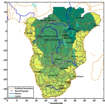
Figure 4 shows the major river basins, being considered in the model. Within the major basins, many model units or “LEWs” have been delineated. Most LEWs represent sub-catchments, however remarks can be made about a few LEWs: the major lakes and reservoirs in our target area, the Zambezi, have also been separately delineated. These are Lake Kariba, Lake Cahora-Bassa and Lake Nyasa (also known as Lake Malawi). The flow behaviour in the upper Nile is very much dependent on the water level in lake Victo-ria. Therefore, a LEW has been defined for lake VictoVicto-ria. Runoff from upstream LEWs spill in this lake and down-stream runoff has been generated through a simple outflow relation dependent on the water level. In the Okavango river basins, the Okavango delta has been delineated manually to take into account the surface runoff redistribution which is actually taking place in this delta. Also its neighbouring in-terior basins have been modelled in a purely “vertical” way, meaning that there is no lateral exchange of water between these basins and others (i.e. there are no runoff processes considered). The same holds for the 2 most eastern sub-catchments of the Shebelle sub-model. These basins drain on the salt lake Turkana (North-Kenya – Rift Valley) and there-fore do not produce any runoff to neighbouring catchments. 4.2 Climate input data
For calibration, the model has been forced by data from the Climate Research Unit (CRU) (New et al., 2002). These data consist of fields of global monthly precipitation, wind speed, relative humidity, and 2 m air temperature (minimum, max-imum and mean). All data are given on a 0.5×0.5 degree grid. The grids have been used to compute reference evap-oration numbers, based on the Penman-Monteith equations (Penman, 1948; Monteith, 1981).
These climate data are completely based on ground station records. The spatial coverage is non-homogeneous in time and, therefore, the quality is non-homogeneous in space and time. For that reason, the emphasis of the model calibration was on the overall discharge behaviour (e.g. the behaviour of apparent linear reservoirs and long-term released volumes). We feel that for our application, the use of CRU data is ade-quate. We must underline that the model developed for this study may be used for other purposes, as well, however it is advised to use regional rainfall sources and re-calibrate the
0 5 10 15 20 25 30 35 40 45 50 −35 −30 −25 −20 −15 −10 −5 0 5 10 15 ° longitude ° latitude AFRICA AFRICAN REPUBLIC ANGOLA BOTSWANA BURUNDI CENTRAL
CONGO, REPUBLIC OF THE
ETHIOPIA GABON KENYA LAND LESOTHO MALAWI MOZAMBIQUE NAMIBIA RWANDA SOMALIA SOUTH SWAZI− TANZANIA UGANDA
CONGO, DEM. REPUBLIC
ZAMBIA ZIMBABWE Political boundary Runoff gauge Rivers Lakes
Fig. 2. The Lumped Elementary Watershed model for Southern
Africa as being used in this study. The grey lines represent the delineations of sub-catchments. Large rivers and lakes are indicated in respectively dark and light blue. The major river basins selected for this model are shown in a color gradient from dark-green to yellow. The black dots indicate locations of runoff gauges, from which monthly stream flow records are available and have been used for calibration.
model when it is used for smaller scales than considered in this study.
4.3 Runoff
Monthly runoff data has been obtained from several data sources, among which the Global Runoff Data Centre and the Zambian Department of Water Affairs (Lusaka, Zambia). Anywhere where there was runoff available (sometimes very short time series), it was used to calibrate the model. Gen-erally, parsimonious model structures were applied and most model units were given the same model structure. In gen-eral, it may be expected that the model performs best in re-gions where both the rainfall and runoff gauge network is relatively dense. As can be observed in Fig. 4, many parts of this model remain ungauged. The reliability of modelled storage is for a large part dependent on the correct estimation of the storage thresholds, more specific, the storage capacity of soil moisture. Generated runoff amounts at river outlets have been therefore calibrated in such a way, that at least the total long-term released volumes of runoff are more or less equal to the observed long-term volumes. This is for example done at the outlet of the Congo. While quite some runoff information was available from the Northern parts of
0 10 20 30 40 50 −35 −30 −25 −20 −15 −10 −5 0 5 10 15 ° longitude ° latitude Upper Zambezi 0 10 20 30 40 50 −35 −30 −25 −20 −15 −10 −5 0 5 10 15 ° longitude ° latitude Zambezi 0 10 20 30 40 50 −35 −30 −25 −20 −15 −10 −5 0 5 10 15 ° longitude ° latitude
up. Zambezi & Okavango
0 10 20 30 40 50 −35 −30 −25 −20 −15 −10 −5 0 5 10 15 ° longitude ° latitude
Zambezi & Congo
✍✁✞❆ ✬ ✍✁☎❏ ✜ ✎☎✁✄✁ ❉ ✁✄✁ ✍✁☎✁✄✁ ✍✁☎✁☎✁ ❑✥▲ ▼◆❖◆◗P ❘ ❙ ▲ ▼◆❖◆❚P ▼❯❱P ✽✿✾✂✾✍✾ ❲ ✾✂✾ ❳ ✾✂✾ ✍✁☎✁☎✁ ✎☎✁✄✁ ✟❀✠ ✠ ✎ ✆ ✁✞✝ ✎✄✁☎✁ ☞ ✂✁✡❆
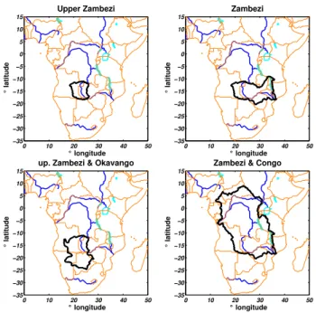
Fig. 3. The four target areas being used in this study (from left to
right, from top to bottom): upper Zambezi, Zambezi, upper Zam-bezi + Okavango, and ZamZam-bezi + Congo.
the Congo, the Southern part (near the Zambezi) remains completely ungauged. Therefore, the LEWs near the Zam-bezi have been given parameter values that were appointed to their neighbouring LEWs located within the Zambezi, where quite some runoff gauges are present and further calibra-tion was applied to match long-term runoff volumes at the Congo’s most downstream runoff gauge.
4.4 Regional water management and wadis
A large challenge in large-scale water balance modelling is the regional lateral interactions that take place between river and surrounding areas, either because of human interference or present topography, geology and climatology. Large dams and lakes may be relatively simple to include in the LEW modelling approach as was described in Sect. 4.2, however information is needed about there operation and general be-haviour (e.g. surface – volume curves and operating rules) to adequately model their water balance. For the applica-tion that is presented in this paper, we feel that a rough es-timation of their water balance should be adequate. In addi-tion, many irrigation schemes are present in Southern Africa, more specifically in the Orange basin, the lower Zambezi and the Incomati. Also wadi areas are present, e.g. in the She-belle river basin, where runoff is generated in the Ethiopian highlands, which ends up in the downstream desert area. The redistribution of surface runoff over either irrigated ar-eas or wadis has been included by spilling a certain amount of runoff in downstream irrigated areas, wadis or wetlands.
For other applications where these interactions are of greater importance, more details about these interactions must be in-cluded in the model.
4.5 LEW model run for GRACE time series
The LEW water storage estimates have been generated us-ing rainfall estimates from the Famine Early Warnus-ing System (FEWS) (Herman et al., 1997). This product is partly satel-lite based and has a resolution of 0.1×0.1◦. The estimates have been lumped over the LEWs to provide a time series from January 2001 until June 2006. The first 2 years of sim-ulation have been taken as warming-up time to stabilize the state variables of the LEW model structures.
5 Results of the error analysis
The analysis has been done for four target areas of different sizes (cf. Fig. 3):
1. upper Zambezi (UZ), 4.7×10⁵km2, 2. Zambezi (Z), 1.3×10⁶km2,
3. upper Zambezi + Okavango (UZO), 1.2×10⁶km2, 4. Zambezi + Congo (ZC), 5.2×10⁶km2.
This has been done in order to investigate the relation be-tween size of the area and amplitude of the bias. The output of the LEW regional hydrological model (cf. Sect. 4) covers the whole area of Southern Africa enabling averaging over the areas in the range of 105−107km2. Gaussian spatial fil-ters with correlation lengths of 600 km, 800 km, and 1000 km have been used and the bias has been computed for each fil-ter.
The output covers the period January 2003 until March 2006. Water storage variations over the area shown in Fig. 4 have been used to compute the bias. A potential contribu-tion to the bias of water storage variacontribu-tions outside this area has been neglected. This is justified because (i) the contri-bution of oceans and atmosphere have already been removed by GFZ prior to the estimation of monthly GRACE models; (ii) the continental areas are outside the significant support of the filter function for the upper Zambezi, Zambezi, and upper Zambezi + Okavango target areas. This does not hold for the Zambezi + Congo target area. Therefore, we expect some errors in the estimated bias for this target area caused by unmodelled mass variations North to the area shown in Fig. 4. We expect that these errors are small as there are little water storage variations in this part of Africa.
5.1 Bias estimate from LEW
Monthly bias estimates have been computed from the output of LEW using Eq. (1). The computations have been done for each target area and choice of the Gaussian filter correlation
Table 1. Amplitudes of the annual bias for different target areas,
computed from LEW model output. Annual amplitudes of (un-filtered) LEW water storage variations and bias-to-signal-ratio are given for comparison.
σ0 bias [mm] f¯0from LEW [mm] rel.bias[%]
Gauss, 1000 km UPZ 73 155 47 Z 61 133 46 UPZO 50 120 42 ZC 22 71 31 Gauss, 800 km UPZ 55 155 35 Z 46 133 35 UPZO 39 120 33 ZC 15 71 21 Gauss, 600 km UPZ 36 155 23 Z 30 133 23 UPZO 28 120 23 ZC 8 71 11
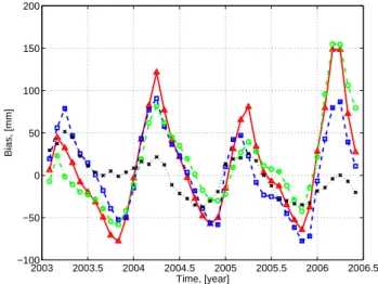
length. Figure 4 shows the bias time series for the four target areas and 1000 km Gaussian smoothing. From the time series of monthly bias values, the amplitude of the annual bias can be computed. The results are shown in Table 1 for each target area and the three Gaussian filters.
The following observations are made:
1. The bias-to-signal-ratio is significant. A comparison of Fig. 4 with 5 shows, that the monthly bias may even ex-ceed the amplitude of the water storage variations (sig-nal). This emphasizes the need to correct GRACE esti-mates of monthly mean water storage variations for the bias introduced by spatial smoothing. Otherwise it will not be possible to calibrate hydrological models using GRACE amplitude estimates.
2. The bias strongly depends on the correlation length of the filter: the smaller the correlation length, the smaller the bias. For instance, moving from 1000 km to 600 km reduces the annual bias amplitude of the upper Zambezi target area from 73 mm to 36 mm, i.e. by about 50%. However, simply reducing the filter correlation length is not the solution to the problem. Even for 600 km, the bias-to-signal-ratio is still very large. Moreover, the choice of a shorter filter correlation length increases the noise in GRACE water storage amplitudes.
3. The bias and the bias-to-signal-ratio depend on the size of the target area: the smaller the target area, the
2003 2003.5 2004 2004.5 2005 2005.5 2006 2006.5 −100 −50 0 50 100 150 200 Time, [year] Bias, [mm]
Fig. 4. Bias as a function of time between January 2003 and March
2006 for four target areas: upper Zambezi (red triangles), Zambezi (blue squares), upper Zambezi + Okavango (green circles) and Zam-bezi + Congo (black x-marks). 1000 km Gaussian smoothing has been used.
larger the bias and the bias-to-signal ratio. For in-stance, for the smallest target area, the upper Zam-bezi (area ≈4.7×10⁵km2), the amplitude of the annual bias is 47% of the annual water storage variation when 1000 km Gaussian smoothing is applied. For the largest area, the Zambezi + Congo, (area ≈5.2×10⁶km2), the annual bias reduces to about 31% of the annual water storage variation.
5.2 Bias-corrected GRACE estimates versus LEW model output
The estimated bias can be used to correct GRACE monthly mean water storage variations. We used 31 release RL03 monthly GRACE gravity field models between January 2003 and March 2006 provided by GFZ. The degree 1 coefficients and the degree 2 zonal coefficient have been excluded from the analysis, which corresponds to the currently adopted pro-cedure. This leads to minor errors in the GRACE monthly mean water storage variations for the target areas consid-ered in this study. From the time-series of monthly grav-ity field models, monthly water storage variations have been computed following the procedure of Swenson and Wahr (2002). These estimates have been corrected then for the bias. For this purpose, the bias estimates, computed from the LEW model output, have been spline interpolated to the time epochs of the monthly GRACE models. Finally, the annual water storage variation has been computed for the biased and bias-corrected GRACE estimates and compared with the an-nual water storage from LEW. The results are summarized in Table 2.
Table 2. Amplitude of the annual water storage variation. [1]: GRACE estimate, [2]: annual bias, [3]: bias-corrected GRACE, [4]: LEW
model output, [5]: difference between bias-corrected GRACE and LEW model output.
target area [1] [2] [3] = [1] + [2] [4] [5] = [3] − [4] Gauss filter, 1000 km UPZ 82 73 155 155 0 Z 83 61 144 133 11 UPZO 68 50 118 120 -2 ZC 33 22 55 71 -16 Gauss filter, 800 km UPZ 102 55 157 155 2 Z 100 46 146 133 13 UPZO 80 39 119 120 -1 ZC 40 15 55 71 -16 Gauss filter, 600 km UPZ 124 36 160 155 5 Z 117 30 147 133 14 UPZO 91 28 119 120 -1 ZC 47 8 55 71 -16
Table 3. Statistics of the differences between GRACE monthly
es-timates and LEW model output before and after bias correction.
area GRACE – LEW GRACEcorr– LEW
min max RMS min max RMS
Gauss filter, 1000 km UPZ 0.4 198.0 68.0 0.3 52.0 25.0 Z 1.4 125.0 48.0 1.5 49.0 27.0 UPZO 1.6 197.0 59.0 1.5 50.0 24.0 ZC 1.5 81.0 35.0 0.0 57.0 20.0 Gauss filter, 800 km UPZ 0.8 174.0 56.0 0.3 61.0 28.0 Z 3.0 106.0 38.0 2.0 58.0 32.0 UPZO 0.0 177.0 52.0 0.3 56.0 26.0 ZC 0.4 80.0 31.0 0.2 66.0 22.0 Gauss filter, 600 km UPZ 0.2 135.0 45.0 7.0 69.0 33.0 Z 1.1 82.0 31.0 1.3 67.0 37.0 UPZO 2.8 147.0 46.0 0.4 59.0 28.0 ZC 1.1 80.0 29.0 1.0 75.0 24.0
A remarkable result is that bias-corrected GRACE esti-mates of the annual and the monthly mean water storage vari-ations fit significantly better with LEW estimates than uncor-rected GRACE estimates (cf. Table 2). For instance, when using 1000 km Gaussian smoothing, the annual difference
re-duces from 73 mm to 0 mm for the upper Zambezi, from 50 to 11 for the Zambezi, from 52 to −2 for the upper Zambezi + Okavango and from 38 to −16 for the Zambezi + Congo area. The annual differences do not depend on the choice of the filter correlation length. Monthly differences between bias-corrected GRACE and LEW are larger than annual dif-ferences, in particular in the wet seasons and for small target areas (cf. Fig. 5).
Table 3 gives some statistical information about the differ-ences between the amplitudes of monthly mean water storage variations from GRACE and LEW model output. It is re-markable that the fit with LEW is the best for a filter correla-tion length of 1000 km; smaller filter correlacorrela-tion lengths lead to larger RMS differences between bias-corrected GRACE and LEW. This can be explained by the fact that filter corre-lation lengths smaller than 1000 km due not sufficiently sup-press the noise in GRACE monthly gravity fields; after bias correction, the noise is still dominant and causes a larger mis-fit between GRACE and LEW. An extreme situation is the Zambezi target area for a 600 km Gaussian filter. After bias correction, the RMS difference between GRACE and LEW
increases from 31 mm to 37 mm!
When a 1000 km Gaussian filter is used, we observe a significant improvement by 44% and 63% of the fit be-tween monthly GRACE and LEW amplitudes after bias cor-rection for all target areas. This is also visible in Fig. 5, which shows the time series of monthly mean water storage variations. The largest difference between LEW and bias-corrected GRACE is attained in spring 2004, whereas the differences in spring 2005 and spring 2006 are significantly
2003 2003.5 2004 2004.5 2005 2005.5 2006 2006.5 −200 −150 −100 −50 0 50 100 150 200 250 Time, year
Water storage variation, [mm]
2003 2003.5 2004 2004.5 2005 2005.5 2006 2006.5 −200 −150 −100 −50 0 50 100 150 200 Time, year
Water storage variation, [mm]
2003 2003.5 2004 2004.5 2005 2005.5 2006 2006.5 −150 −100 −50 0 50 100 150 200 250 Time, year
Water storage variation, [mm]
2003 2003.5 2004 2004.5 2005 2005.5 2006 2006.5 −150 −100 −50 0 50 100 150 Time, year
Water storage variation, [mm]
Fig. 5. Time series of monthly mean water storage variations over the target areas: From left to right and top to bottom: upper Zambezi,
Zambezi, upper Zambezi + Okavango, and Zambezi + Congo. A 1000 km Gaussian filter has been used. Black triangles: unfiltered LEW; blue x-marks: biased GRACE; red boxes: bias-corrected GRACE.
smaller. The reason for the large difference in spring 2004 is not clear yet. It could be attributed to either the LEW model or the GRACE data. For instance, a poor quality of rainfall input data from the beginning of 2004 could cause significant errors in the LEW model output. This would also propagate into the computed bias. Alternatively, it is possible that GRACE did not capture the water storage variation over the target areas very well in spring 2004, due to a poor orbit geometry (Winsemius et al., 2006b). This would cause an additional bias in GRACE monthly amplitudes, which can-not be corrected for.
The maximum difference between bias-corrected GRACE and LEW monthly amplitudes (57 mm for 1000 km Gaussian smoothing) is observed in the Zambezi + Congo area, which is the largest target area. At the first glance, this is unex-pected as the bias is the smallest for this area and the quality of GRACE should improve with increasing size of the tar-get area. We explain this with the poorer performance of the
LEW model, which does not provide good estimates of water storage variations in the areas North to the Zambezi + Congo target area (cf. Figs. 4 and 3). This information is needed to get a good estimate of the bias, as mass variations outside the target area contribute to the bias according to Eq. (1). The poorer performance of LEW may be a consequence of the poor coverage of this area with gauge stations, which causes a bias in the rainfall data.
Chen et al. (2007) report significant phase shifts up to 10 deg for some areas after spatial smoothing is applied. For the four target areas in Southern Africa, the phases of the water storage variations from the bias-corrected GRACE and (un-filtered) LEW model output fit quite well. The annual phase difference is maximum for the upper Zambezi + Okavango target area (0.25 months or 7.5 deg); for the other target ar-eas, the annual phase difference is below 0.1 months (or 3 deg).
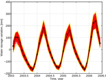
2003 2003.5 2004 2004.5 2005 2005.5 2006 2006.5 −200 −100 0 100 200 300 400 Time, year
Water storage variation, [mm]
Fig. 6. Water storage variations (in red) averaged over the upper
Zambezi basin from the Monte Carlo simulation (200 realizations, 30% noise in rainfall numbers). Mean water storage is given in black.
5.3 Bias, bias uncertainty, and the role of the hydrological model
In this section, we want to address two questions:
1. The computation of the bias in GRACE monthly mean water storage variations requires knowledge about the water storage variations inside and outside the target area. This information is, of course, not available as otherwise there would be no need to use GRACE. In practice, only some a priori information about the water storage variations may be available, e.g. from a hydro-logical model. Uncertainties in the a priori information propagates into the estimated bias. Therefore, the ques-tion is how changes in the hydrological model output propagate into the bias estimates.
2. In the analysis done before, the same hydrological model (LEW) is used for bias computation and for com-parison with GRACE. We concluded that after bias cor-rection, the fit between LEW and GRACE improves sig-nificantly. Therefore, one may ask whether the fit is less if another hydrological model is used to compute the bias.
A thorough answer to the first question requires an as-sessment of the uncertainty of the LEW hydrological model. This is extremely complex and out of the scope of this study. Therefore, a more simplistic approach is followed, which is based on the fact that the rainfall data are the most signif-icant (but not the only) source of uncertainty of the output of LEW for South Africa. Therefore, we generated a series of alternative water storage variations over the target areas
2003 2003.5 2004 2004.5 2005 2005.5 2006 2006.5 −150 −100 −50 0 50 100 150 200 Time, year Bias, [mm]
Fig. 7. Time variable bias (in green) averaged over the upper
Zam-bezi target area from a Monte Carlo simulation (200 realizations, 30% noise in rainfall numbers). Mean bias is given in black.
using a Monte-Carlo simulation. This series have been ob-tained by changing the input rainfall data to LEW randomly. That is, the rainfall data were superimposed by a zero mean Gaussian white noise with a standard deviation of 30% of the rainfall numbers. 200 noise realizations have been generated for each time step. For each set of rainfall data, the LEW model has been run, which yields water storage variation es-timates for the area shown in Fig. 4 for the period January 2003 until March 2006. These estimates have been used to compute a time series of the bias for the period January 2003 until March 2006. From the 200 realizations, a mean bias and a RMS bias have been computed for each time step.
Figures 6 and 7 show the 200 monthly mean water storage variations and the estimated bias time series, respectively, for the upper Zambezi target area. The RMS bias shows a signif-icant yearly pattern, which is in phase with the rainfall pat-tern. That is, the largest RMS values are attained during the wet season, i.e. in spring each year. In fall, the uncertainties are much smaller, because there is almost no rainfall.
For the upper Zambezi area and a 1000 km Gaussian filter, the maximum RMS bias is attained in spring 2006 (27 mm) (cf. Fig. 8); the annual RMS bias is 15 mm. This is much smaller than the 73 mm difference of the annual amplitude of water storage variation between LEW and (uncorrected) GRACE (cf. Table 2, UPZ, column [1] and [4]). Therefore, the Monte Carlo experiment indicates that even relatively un-certain information about mass variations is helpful to reduce the bias significantly.
In order to address the second question, we repeat the complete data analysis with the global hydrological model CPC-LDAS, and compared the results with the ones ob-tained with the LEW model. The land data assimilation sys-tem (LDAS) is one of the land surface models developed at
20035 2003.5 2004 2004.5 2005 2005.5 2006 2006.5 10 15 20 25 30 Time, year Bias rms, [mm]
Fig. 8. RMS of the monthly bias caused by 30% noise in
rain-fall numbers for the upper Zambezi target area. 1000 km Gaussian smoothing applied.
NOAA Climate Prediction Center (CPC). It is forced by ob-served precipitation, derived from CPC daily and hourly pre-cipitation analysis, downward solar and long-wave radiation, surface pressure, humidity, 2-m temperature and horizontal wind speed from NCEP reanalysis. The output consists of soil temperature and soil moisture in four layers below the ground. At the surface, it includes all components affecting energy and water mass balance, including snow cover, depth, and albedo. The data for the CPC-LDAS model are freely available on the INTERNET (CPC, a,b). No data have been found after December 2005. Therefore, the comparison with LEW covers the period January 2003 until December 2005. The CPC-LDAS model has also been used in other GRACE studies, e.g. in Swenson et al. (2003); Wahr et al. (2004).
The following differences of water storage variations have been computed for the period January 2003 until December 2005:
– LEW minus (uncorrected) GRACE (referred to as
LEW-GRACE)
– LEW minus (bias-corrected) GRACE; the bias is
com-puted using LEW (referred to as LEW-GRACE/LEW)
– LEW minus (bias-corrected) GRACE; the bias is
computed using CPC-LDAS (referred to as LEW-GRACE/CPC)
– CPC-LDAS minus (uncorrected) GRACE (referred to
as CPC-GRACE)
– CPC-LDAS minus (bias-corrected) GRACE; the bias
is computed using CPC-LDAS (referred to as LEW-GRACE/CPC) 2003 2003.5 2004 2004.5 2005 2005.5 2006 −80 −60 −40 −20 0 20 40 60 80 Time, [year] Bias, [mm]
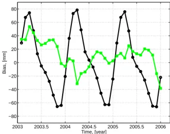
Fig. 9. Time series of bias estimates computed on the basis of the
CPC-LDAS hydrological model (black circles) and the differences between the bias from CPC-LDAS and LEW (green squares) for the Upper Zambezi target area.
– CPC-LDAS minus (bias-corrected) GRACE; the bias
is computed using LEW (referred to as CPC-GRACE/LEW)
The main results of this comparison are shown in Fig. 9 (comparison of the bias computed from LEW and CPC-LDAS, respectively, for the Upper Zambezi target area), Figs. 10 and 11 (time series of differences between LEW, CPC-LDAS, and GRACE for the Upper Zambezi target area), and Table 4 (RMS differences between LEW, CPC-LDAS, and GRACE for all target areas). They can be sum-marized as follows:
1. Bias estimates computed from LEW and CPC-LDAS show significant differences (cf. Fig. 9). For the period January 2003 until December 2005, the largest differ-ence is 55 mm. It is attained during wet periods, i.e. when strong rainfall occurs. The RMS difference is about 15 mm. On the other hand, these differences are much smaller than the bias itself.
2. The differences LEW-GRACE/LEW and
CPC-GRACE/CPC are significantly smaller than LEW-GRACE and CPC-LEW-GRACE, respectively. The same holds for the differences LEW-GRACE/CPC and CPC-GRACE/LEW compared with LEW-GRACE and CPC-GRACE, respectively. This indicates that bias correction really works for the target areas subject to this study.
3. The fit of a hydrological model with bias-corrected GRACE is overoptimistic if the same hydrological model is used to compute the bias. This is evident if one
2003.5 2004 2004.5 2005 2005.5 2006 −100 −80 −60 −40 −20 0 20 40 60 80 100 Time, [year]
Water storage variation, [mm]
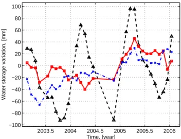
Fig. 10. Differences of water storage variations from LEW and
GRACE for the period January 2003 until December 2005. Up-per Zambezi target area. Gaussian filter with 1000 km correlation length. Black triangles: LEW – GRACE; red squares: LEW – GRACE/LEW; blue crosses: LEW-GRACE/CPC
2003.5 2004 2004.5 2005 2005.5 2006 −100 −50 0 50 100 Time, [year]
Water storage variation, [mm]
Fig. 11. Differences of water storage variations from CPC-LDAS
and GRACE for the period January 2003 until December 2005. Up-per Zambezi target area. Gaussian filter with 1000 km correlation length. Black triangles: LDAS – GRACE; red squares: CPC-LDAS – GRACE/CPC; blue crosses: CPC-CPC-LDAS – GRACE/LEW.
compares the RMS difference between GRACE/LEW and GRACE/CPC (which is in fact the difference of the bias as computed from LEW and CPC-LDAS), with the RMS difference between LEW-GRACE/LEW and CPC-GRACE/CPC. In this sense, one can say that the estimated bias is “biased” towards the hydrological model used. This makes it very difficult to decide what hydrological model better fits GRACE (or vice versa),
Table 4. Statistics of the differences between LEW and GRACE,
and CPC and GRACE monthly estimates of the water storage. A Gaussian filter with 1000 km has been used.
RMS
diff. UPZ Z UPZO ZC
Gauss filter, 1000 km LEW – GRACE 54.0 41.0 41.0 36.0 LEW – GRACE/LEW 22.0 26.0 18.0 19.0 LEW – GRACE/CPC 28.0 22.0 29.0 24.0 CPC – GRACE 65.0 41.0 72.0 34.0 CPC – GRACE/CPC 28.0 40.0 51.0 22.0 CPC – GRACE/LEW 40.0 56.0 57.0 35.0
and to draw conclusions about the noise in GRACE and hydrological model estimates of water storage varia-tions after bias correction.
4. The difference LEW-GRACE is always smaller than the difference CPC-GRACE. That is, (uncorrected) GRACE better fits the LEW model output than the CPC-LDAS model output.
5. The difference LEW-GRACE/LEW is always smaller than CPC-GRACE/CPC.
6. The difference LEW-GRACE/CPC is always smaller than CPC-GRACE/LEW.
Items 4, 5, and 6 may be seen as an indicator of the supe-rior quality of LEW compared with CPC-LDAS for the four target areas.
6 Conclusions
Spatial smoothing of GRACE monthly gravity field models introduces a significant bias in GRACE-estimated monthly mean water storage variations. For the four target areas con-sidered in this study, the bias attains values between 50–70% of the total water storage variation. This confirms estimates reported in previous studies for other areas, (e.g. Chen et al., 2007). For most target areas in the world, GRACE always underestimates the amplitudes of monthly mean water stor-age variations.
The bias strongly depends on the amplitude of the water storage variation inside and outside the target areas. More-over, the size and shape of the target area also influence the amplitude of the bias. Generally, the larger the target area, the smaller the bias.
Without bias correction, it is hardly possible to enhance hydrological models using GRACE. To compute the bias, a
priori information about the mass variations inside and out-side the target area is needed. This information can be pro-vided for instance by hydrological models. Whether GRACE itself can be used as source of information in an iterative ap-proach to bias estimation has to be investigated. In this study, the output of a regional hydrological model has been used successfully to estimate the bias. After bias correction, the annual amplitude differences of GRACE and regional hydro-logical model reduce to some millimeters.
Monthly amplitude differences may be significantly larger than annual differences, in particular during wet periods. There are two potential explanations: first of all, the LEW model does not perform well during these periods; this also effects the estimated bias. Secondly, GRACE does not cap-ture the monthly water storage variation very well, which is caused by an unfavorable orbit geometry. However, the ex-ceptionally large 30 mm amplitude difference for the Zam-bezi + Congo target area in spring 2004 is likely a result of a poor performance of the LEW model to estimate mass varia-tions for the area North to the Zambezi + Congo target area.
We do not observe significant phase differences between GRACE and LEW. The maximum phase difference is 0.25 month (i.e. 7.5 deg) for the upper Zambezi + Okavango area; the phase difference for the other target areas is below 0.1 month (i.e. 3 deg).
The RMS of the bias due to 30% noise in rainfall num-bers vary between 5 mm and 27 mm. Averaged over the pe-riod between January 2003 until March 2006, this is about 20% of the amplitude of the water storage variation. The as-sumption of 30% noise in rainfall data is rather pessimistic, although there are other contributors to the error budget of LEW water storage estimates, which propagate into the esti-mated bias. Therefore, it should be possible to obtain good estimates of the bias even if the quality of the a priori in-formation about mass variations inside and outside the target area is relatively poor. The question of bias estimability using a priori information about mass variations, however, depends on the location of the target area and has to be addressed on a case-by-case basis.
For the target areas subject to this study, bias correc-tion improves significantly the quality of GRACE estimates of water storage variations, independently whether LEW or CPC-LDAS is used to compute the bias. As bias estimates are biased towards the hydrological model used to compute the bias, the fit between a hydrological model and bias-corrected GRACE is too optimistic.
The study limits to the application of isotropic Gaussian smoothing. When using other filter functions, e.g. non-isotropic filters or Wiener filters, the bias is likely to be smaller. Nevertheless, the need to apply a bias correction is still there. The ability to compute the bias depends on the location of the target area and the availability of a priori in-formation about mass variations inside and outside the target area. The question whether GRACE can be used in an
iter-ative approach to provide this information as alterniter-ative to hydrological models is left open for future studies.
Appendix A
Suppose the function f describes the monthly mean mass variations on Earth. Let σ0 be our target area (e.g. a river basin) and σRthe mean surface of the Earth, represented as a sphere with radius R. The mean value of the function f over σ0is ¯ f0= 1 σ0 Z σ0 f dσR. (A1)
Introducing the characteristic function of the target area
χ = (4π R2
σ0 in σ0
0 in σR− σ0 , we can write Eq. (A1) as
¯ f0= 1 4π R2 Z σR f χ dσR. (A2)
The true monthly mean mass variation function f is of course unknown; from GRACE monthly gravity field solu-tions, we can obtain an estimate ˆf . With
f = ˆf + εf, this estimate is ¯ f0= 1 4π R2 Z σR ˆ f χ dσR+ 1 4π R2 Z σR εfχ dσR. (A3)
The second term on the right-hand side of Eq. (A3) describes the error of the GRACE estimate of the monthly mean mass variation averaged over the target area. In reality, this term is very large, and the standard procedure to reduce it is to apply spatial smoothing with a filter Ws,
ˆ fs = 1 4π R2 Z σR ˆ f WsdσR.
Correspondingly, ˆfs instead of ˆf is used to compute the monthly mean mass variation averaged over the target area according to ˆ¯ f0= 1 4π R2 Z σR ˆ fsχ dσR.
Often (but not necessarily), the spatial filter (smoother) Wsis an isotropic function on the sphere, e.g. a Gaussian. The true monthly mean mass variation averaged over the target area is
¯ f0= ˆ¯f0 + 1 4π R2 Z σR (f − fs)χ dσR+ 1 4π R2 Z σR εfsχ dσR, (A4)
where fs= ˆfs+εfs and εfs is the error of ˆfs. The first term
on the right-hand side of Eq. (A4) is the estimate we obtain from GRACE monthly gravity models. The last two terms describe the error. The first error term is the error introduced by the spatial smoothing; the second error term describes how GRACE errors propagate into the smoothed mass vari-ation function ˆfs. The spatial smoothing only makes sense (i.e. is successful) if | Z σR (f − fs)χ dσR+ Z σR εfsχ dσR| < | Z σR εf χ dσR|. With W := 1 4π R2 Z σR WSχ dσR,
it can easily be shown that ˆ¯ f0= 1 4π R2 Z σR ˆ f W dσR, (A5) and ¯ f0= ˆ¯f0 + 1 4π R2 Z σR f (χ − W ) dσR+ 1 4π R2 Z σR εfW dσR. (A6) The second term on the right-hand side of Eq. (A6),
¯ε0:= 1 4π R2 Z σR f (χ − W ) dσR, (A7)
is the bias in the monthly mean mass variation averaged over the target areas that is caused by spatial smoothing. The bias can be interpreted as the error we introduce when using the filter W instead of the characteristic function χ . That is, us-ing W reduces GRACE-related errors, but introduces at the same time a bias in the monthly mean mass variation esti-mate. To balance these errors is the subject of the choice of an optimal filter. This is not addressed here; for details about the optimal choice of a filter, we recommend (Swenson and Wahr, 2002) and (Han et al., 2005). To analyze the bias ¯ε0, we first write f = ( f0 in σ0 fl in σR− σ0 , and obtain a decomposition of ¯ε0into two parts:
¯ε0= 1 4π R2 Z σ0 f0(χ − W ) dσR + 1 4π R2 Z σR−σ0 fl(χ − W ) dσR. (A8)
The type 2 error can be re-written, when taking into account that χ =0 in σR−σ0. Then, Z σR−σ0 fl(χ − W ) dσR= − Z σR−σ0 flW dσR.
Now, the true monthly mean mass variation averaged over the target area can be written as
¯
f0= ˆ¯f0+ ε1+ ε2+ ε3,
wherefˆ¯0is the GRACE estimate (cf. Eq. (A5)), and ε1= 1 4π R2 Z σ0 f0(χ − W ) dσR ε2= − 1 4π R2 Z σR−σ0 flW dσR ε3= 1 4π R2 Z σR εfW dσR.
describe the errors, with the bias ¯ε0=ε1+ε2.
Many authors account for the errors in the estimated am-plitudes of the monthly mean water storage variation over the target area, by changing the correlation length of the fil-ter Wssuch that the GRACE water storage amplitudes fit best in a least-squares sense the amplitudes of a global hydrolog-ical model on a global scale. For a Gaussian filter function, this gives a filter correlation length of about 800 km for the routinely used global hydrological models GLDAS. This ap-proach is certainly weaker than the apap-proach by Velicogna and Wahr (2006), although in this way, errors in the global hydrological model may average out a little bit. Anyway, the best one can obtain then is a global scale factor; scale factors for specific regions of interest may significantly differ from the global one.
Velicogna and Wahr (2006) followed another approach. They introduced a scale factor λ, defined as
λ = R σRf χ dσR R σRf W dσR ,
and obtained an estimate ˆλ of λ assuming that the mass vari-ation function f is f = ( h = constant in σ0 0 in σR− σ0 .
The function h was assumed to be a layer of water with thick-ness 1 cm distributed over the target area. Then,
ˆλ = R 1 σ0W dσR
.
Thereafter, the estimate ˆλfˆ¯0 was used as scale-corrected GRACE estimate of the monthly mean mass variation av-eraged over the target area. This simple approach of correct-ing GRACE water storage amplitudes for the bias is correct if there are no mass variations outside the target area. Only then, the scale factor does not depend on the amplitude of the mass variation inside the target area and the scale factor can
properly be determined by the assumption of a homogeneous mass layer of any thickness. However, if there are mass vari-ations outside the target area, the estimated scale factor is erroneous. Then, the exact scale factor depends among oth-ers on the amplitude of the mass variation inside and outside the target area as shown in Eq. (1).
Acknowledgements. We would like to thank two anonymous
re-viewers for their valuable and very detailed comments, which helped us improving the manuscript significantly. Please refer to the online discussion: www.hydrol-earth-syst-sci-discuss.net/3/3557/ 2006/
The project is supported by the Dutch Organization for Scientific Research (NWO) and the Water Research Center Delft (WRCD).
The support is greatly acknowledged. We are thankful for the
GRACE data provided by GeoForschungsZentrum Potsdam (GFZ, Germany’s National Research Centre for Geosciences); in partic-ular we want to thank Dr. Frank Flechtner for his support to this study. The computations have been done partly on the SGI Origin 3800 and SGI Altix 3700 super computers in the framework of the grant SG-027, which is provided by “Stichting Nationale Comput-erfaciliteiten” (NCF).
We greatly appreciate the collaboration with mr. Chris Chileshe from the Department of Water Affairs (Lusaka, Zambia), who has provided us with considerable discharge records of several locations within the Zambezi river basin. Second, we are grateful for the discharge records, gathered and provided by the Global Runoff Data Centre. Finally we would like to thank the Netherlands Organisation for Scientific Research for their contribution to our research.
Edited by: G. Pegram
References
http://www.csr.utexas.edu/research/ggfc/dataresources.html, a. ftp://ftp.csr.utexas.edu/pub/ggfc/water/CPC/, b.
Chen, J. L., Rodell, M., Wilson, C., and Famigletti, J. S.: Low de-gree spherical harmonic influences on Gravity Recovery and Cli-mate Experiment (GRACE) water storage estiCli-mates, Geophys. Res. Lett., 32, L14 405, doi:10.1029/2005GL022964, 2005a. Chen, J. L., Wilson, C. R., Famiglietti, J. S., and Rodell, M.:
Spa-tial sensitivity of the Gravity Recovery and Climate Experiment GRACE time-variable gravity observations, J. Geophys. Res., 110, B08408, doi:10.1029/2004JB003536, 2005b.
Chen, J. L., R.Wilson, C., Famigletti, J. S., and Rodell, M.: Atten-uation effect on seasonal basin-scale water storage change from GRACE time-variable gravity, J. Geodesy, 81, 237–245, 2007. Fenoglio-Marc, L., Kusche, J., and Becker, M.: Mass variation in
the Mediterranean Sea from GRACE and its validation by altime-try, steric and hydrology fields, Geophys. Res. Lett., 33, L19606, doi:10.1029/2006GL026851, 2006.
Han, S. C., Shum, C. K., Jekeli, C., Kuo, C. Y., Wilson, C. R., and Seo, K. W.: Non-isotropic filtering of GRACE temporal gravity for geophysical signal enhancement, Geophys. J. Int., 163, 18– 25, 2005.
Herman, A., Kumar, V. B., Arkin, P. A., and Kousky, J. V.: Ob-jectively determined 10-day African rainfall estimates created for Famine Early Warning Systems, Int. J. Remote Sensing, 18, 2147–2159, 1997.
Jekeli, C.: Alternative methods to smooth the Earth’s gravity field., Tech. rep., Department of Geodetic Science, Ohio State Univer-sity, Columbus, Ohio, 1981.
Klees, R., Zapreeva, E. A., Savenije, H. H. G., and Winsemius, H. C.: Monthly mean water storage variations by the combina-tion of GRACE and a regional hydrological model: applicacombina-tion to the Zambezi River Basin, Proceedings Dynamic Planet 2005, Monitoring and Understanding a Dynamic Planet with Geodetic and Oceanographic Tools, 2006.
Monteith, J. L.: Evaporation and surface temperature, Q. J. R. Me-teorol. Soc., 107, 1–27, 1981.
New, M., Lister, D., Hulme, M., and Makin, I.: A high-resolution data set of surface climate over global land areas, Clim. Res., 21, 1–25, 2002.
Penman, H. L.: Natural evaporation from open water, bare soil and grass, Proc. Roy. Soc. London, A193, 120–145, 1948.
Swenson, S. and Wahr, J.: Methods for inferring regional surface-mass anomalies from Gravity Recovery and Climate Experiment (GRACE) measurements of time-variable gravity, J. Geophys. Res., 107, 2193, doi:10.1029/2001JB000576, 2002.
Swenson, S. and Wahr, J.: Post-processing removal of correlated errors in GRACE data, Geophys. Res. Lett., 33, L08 402, doi: 10.1029/2005GL025285, 2006.
Swenson, S., Wahr, J., and Milly, P. C. D.: Estimated accuracies of regional water storage variations inferred from the Gravity Re-covery and Climate Experiment (GRACE), Water Resour. Res., 39, 1223, doi:10.1029/2002WR001808, 2003.
Velicogna, I. and Wahr, J.: Measurements of time-variable gravity show mass loss in Antarctica, Science, 311, 1754–1756, 2006. Wahr, J., Molenaar, M., and Bryan, F.: Time variability of the
earth’s gravity field: Hydrological and oceanic effects and their possible detection using GRACE, J. Geophys. Res., 103, 30 205– 30 230, 1998.
Wahr, J., S.Swenson, Zlotnicki, V., and Velicogna, I.: Time-variable gravity from GRACE: First results, Geophys. Res. Lett., 31, L11 501, doi:10.1029/2004GL019779, 2004.
Wahr, J., Swenson, S., and Velicogna, I.: Accuracy of GRACE mass estimates, Geophys. Res. Lett., 33, L06401, doi:10.1029/ 2005GL025305, 2006.
Winsemius, H. C., Savenije, H. H. G., Gerrits, A. M. J., Zapreeva, E. A., and Klees, R.: Comparison of two model approaches in the Zambezi river basin with regard to model confidence and identi-fiability, Hydrol. Earth Syst. Sci., 10, 339–352, 2006a.
Winsemius, H. C., Savenije, H. H. G., van de Giessen, N., van de Hurk, B., Zapreeva, E. A., and Klees, R.: Valida-tion of GRACE temporal signature with a hydrological model of the upper Zambezi, Water Resour. Res., 42, W12201, doi:10.1029/2006WR005192, 2006b.
![Table 2. Amplitude of the annual water storage variation. [1]: GRACE estimate, [2]: annual bias, [3]: bias-corrected GRACE, [4]: LEW model output, [5]: difference between bias-corrected GRACE and LEW model output.](https://thumb-eu.123doks.com/thumbv2/123doknet/14794009.602775/9.892.252.636.149.476/table-amplitude-storage-variation-estimate-corrected-difference-corrected.webp)