HAL Id: hal-00298426
https://hal.archives-ouvertes.fr/hal-00298426
Submitted on 21 Sep 2006HAL is a multi-disciplinary open access
archive for the deposit and dissemination of sci-entific research documents, whether they are pub-lished or not. The documents may come from teaching and research institutions in France or abroad, or from public or private research centers.
L’archive ouverte pluridisciplinaire HAL, est destinée au dépôt et à la diffusion de documents scientifiques de niveau recherche, publiés ou non, émanant des établissements d’enseignement et de recherche français ou étrangers, des laboratoires publics ou privés.
Assimilation of ocean colour data into a Biochemical
Flux Model of the Eastern Mediterranean Sea
G. Triantafyllou, G. Korres, I. Hoteit, G. Petihakis, A. C. Banks
To cite this version:
G. Triantafyllou, G. Korres, I. Hoteit, G. Petihakis, A. C. Banks. Assimilation of ocean colour data into a Biochemical Flux Model of the Eastern Mediterranean Sea. Ocean Science Discussions, European Geosciences Union, 2006, 3 (5), pp.1569-1608. �hal-00298426�
OSD
3, 1569–1608, 2006Data assimilation into Eastern Mediterranean Ecosystem Model G. Triantafyllou et al. Title Page Abstract Introduction Conclusions References Tables Figures J I J I Back Close
Full Screen / Esc
Printer-friendly Version
Interactive Discussion Ocean Sci. Discuss., 3, 1569–1608, 2006
www.ocean-sci-discuss.net/3/1569/2006/ © Author(s) 2006. This work is licensed under a Creative Commons License.
Ocean Science Discussions
Papers published in Ocean Science Discussions are under open-access review for the journal Ocean Science
Assimilation of ocean colour data into a
Biochemical Flux Model of the Eastern
Mediterranean Sea
G. Triantafyllou1, G. Korres1, I. Hoteit2, G. Petihakis1, and A. C. Banks1
1
Hellenic Centre for Marine Research, Anavissos, Greece
2
Scripps Institution of Oceanography, La Jolla, CA, USA
Received: 2 August 2006 – Accepted: 10 September 2006 – Published: 21 September 2006 Correspondence to: G. Triantafyllou ([email protected])
OSD
3, 1569–1608, 2006Data assimilation into Eastern Mediterranean Ecosystem Model G. Triantafyllou et al. Title Page Abstract Introduction Conclusions References Tables Figures J I J I Back Close
Full Screen / Esc
Printer-friendly Version
Interactive Discussion Abstract
Within the framework of the European MFSTEP project, an advanced multivariate se-quential data assimilation system has been implemented to assimilate real chloro-phyll data from the Sea-viewing Wide Field-of-view Sensor (SeaWiFS) into a three-dimensional biochemical model of the Eastern Mediterranean. The physical ocean
5
is described through the Princeton Ocean Model (POM) while the biochemistry of the ecosystem is tackled with the Biochemical Flux Model (BFM). The assimilation scheme is based on the Singular Evolutive Extended Kalman (SEEK) filter, in which the error statistics were parameterized by means of a suitable set of Empirical Orthogonal Func-tions (EOFs). A radius of influence was further selected around every data point to limit
10
the range of the EOFs spatial correlations. The assimilation experiment was performed for one year over 1999 and forced with ECMWF 6 hour atmospheric fields. The accu-racy of the ecological state identification by the assimilation system is assessed by the relevance of the system in fitting the data, and through the impact of the assimilation on non-observed biochemical processes. Assimilation of SeaWiFS data significantly
15
improves the forecasting capability of the BFM model. Results, however, indicate the necessity of subsurface data to enhance the controllability of the ecosystem model in the deep layers.
1 Introduction
The Mediterranean Sea is divided by prominent discontinuities into sub-basins
decou-20
pling hydrodynamics and ecological conditions. The high evaporation, low rainfall and river runoff, in conjunction with the outflow of the bottom layer at Gibraltar, result in an oligotrophic gradient toward the east. The observed oligotrophy is thought to be due to low phosphorus concentrations (decreasing from west to east) limiting phytoplankton and bacterial growth (Krom et al., 1992). The state of the art in forecasting the
Mediter-25
ranean Sea circulation is an operational system based on physical components. While 1570
OSD
3, 1569–1608, 2006Data assimilation into Eastern Mediterranean Ecosystem Model G. Triantafyllou et al. Title Page Abstract Introduction Conclusions References Tables Figures J I J I Back Close
Full Screen / Esc
Printer-friendly Version
Interactive Discussion these systems exist for ocean physics, the scientific knowledge and technological
ca-pacity to construct such a system for the ecosystem is currently lacking. The three dimensional modelling of marine ecosystems is lagging behind the modelling of ma-rine physics, because it requires robust hydrodynamic models and adequate comput-ing resources. Furthermore, to achieve accurate predictive capabilities, deterministic
5
ecosystem models need to be adjusted with biological, physical and chemical data at relevant space-time scales. The framework of data assimilation provides the ap-propriate tools for improving models’ agreement with data and for assessing them in predictive mode. Although assimilation systems for meteorological and oceanic models are well established, the use of data assimilation techniques with marine ecosystem
10
models is far less developed. An assimilation system is composed of two basic compo-nents, an observing system and a numerical model complemented with a data assimi-lation scheme that can efficiently extract the reliable information from the observations to optimally initialize the forecast. One of the only synoptic data sources on the state of coastal and pelagic ecosystems comes from “ocean colour” satellite remote sensing
15
(Platt et al., 1995). Since the launch of the Coastal Zone Colour Scanner on the Nim-bus 7 satellite in 1978, satellite borne ocean colour sensors have become the standard tool for determining distributions of phytoplankton and other biochemical parameters in the ocean (IOCCG, 1999). Satellite data benefits from a high temporal resolution with repeat coverage of the same area of the sea surface on a daily basis. The quality of
20
the data is, however, limited by the ability of remote sensing of ocean colour, through the analysis of ocean leaving radiance, to yield information on water-quality parame-ters such as phytoplankton pigments (more precisely chlorophyll a and phaeophytin a), suspended sediment, and yellow substance (gelbstoff) in the euphotic layer (Tassan, 1994). Chlorophyll-a is one of the key parameters of the ecosystem model used here
25
(Biochemical Flux Model–BFM) and therefore the appropriate use of satellite data may guide the modeling and forecasting process closer to realistic conditions. However, the key to the use of these data in predictive/forecasting research using hydrodynamic and ecosystem modeling relies on two premises. Firstly, the availability of accurate
OSD
3, 1569–1608, 2006Data assimilation into Eastern Mediterranean Ecosystem Model G. Triantafyllou et al. Title Page Abstract Introduction Conclusions References Tables Figures J I J I Back Close
Full Screen / Esc
Printer-friendly Version
Interactive Discussion chlorophyll-a estimates from the original spectral data over the area of interest using
well calibrated retrieval algorithms, and secondly that the precise implementation of advanced assimilation techniques capable of handling the satellite data is achievable. In the domain of marine ecology, early studies used four-dimensional variational data assimilation techniques for estimating the poorly known parameters in the model. Such
5
techniques basically seek for the unknown parameters that minimize the misfit between model simulations and data, e.g. the adjoint method (Fennel et al., 2001; Friedrichs, 2001; Gunson et al., 1999; Lawson et al., 1996; Spiitz et al., 1998; Vallino, 2000), di-rect minimization methods (Fasham and Evans, 1995; Prunet et al., 1996), and Monte Carlo methods (Harmon and Challenor, 1996; Matear, 1995). Recently, focus shifted
10
toward the use of Kalman filter based sequential assimilation techniques to directly compute estimates of the system state, as these methods allow for efficient handling of the model uncertainties while intermittently adjusting the model trajectory each time new observations are available (Ghil and Malanotte-Rizzoli, 1991). Taking into account (even partially) the model error is a key step for building a successful ecosystem
assim-15
ilation system because of significant uncertainties in the current ecological models. For instance, Anderson et al. (2000) used optimal interpolation to assimilate both physical and biological data into a mesoscale-resolution 3-D ocean model. Allen et al. (2002) and Natvik and Evensen (2002) demonstrated the effectiveness of the well-known en-semble Kalman filter for data assimilation with a 1-D, three-component model. The
Sin-20
gular Evolutive Extended Kalman (SEEK) filter, which is a suboptimal extended Kalman (EK) filter developed by Pham et al. (1997), was particularly popular and successfully implemented in several marine ecosystem data assimilation studies. The SEEK filter operates with low-rank matrices to avoid the prohibitive computational cost of the EK filter (Cane et al., 1996; Fukumori and Malanotte-Rizzoli, 1995), while only adjusting
25
the model forecast in the directions of error growth. It further supports different degrees of simplifications in the evolution of its “correction directions” at a minimal loss of per-formance (Hoteit et al., 2002, 2004). Carmillet et al. (2001) used the SEEK filter with an invariant set of Empirical Orthogonal Functions (EOFs) correction directions to
OSD
3, 1569–1608, 2006Data assimilation into Eastern Mediterranean Ecosystem Model G. Triantafyllou et al. Title Page Abstract Introduction Conclusions References Tables Figures J I J I Back Close
Full Screen / Esc
Printer-friendly Version
Interactive Discussion similate pseudo-ocean colour data into a 3-D physical–biochemical model of the North
Atlantic Ocean. Hoteit et al. (2003) used the same filter with a 1-D complex ecosys-tem model of the Cretan Sea assimilating real observations of oxygen and nitrate and validating the filter with independent chlorophyll data. Triantafyllou et al. (2003) imple-mented the interpolated version of the SEEK filter in a three dimensional ecosystem
5
model of the Cretan Sea. In the same area, (Hoteit et al., 2005) successfully tested the SEEK filter with semi-evolutive correction directions composed of global and lo-cal EOFs. The reader is referred to Triantafyllou et al. (2005) for a review on the implementation of the SEEK filter and its variants in shelf and regional areas of the Mediterranean Sea. One of the major goals of the Mediterranean ocean Forecasting
10
System (MFS) project during the second phase (2003–2006), named Toward Environ-mental Predictions (MFSTEP), was the development of numerical forecasting systems at basin scale and for regional areas. Within the framework of this project, our work consists of implementing the SEEK filter to assimilate Sea viewing Wide Field of view Sensor (SeaWiFS) data into a coupled physical (Princeton Ocean Model)–biological
15
(Biochemical Flux Model) model of the Eastern Mediterranean, developed during the first phase of the MFSTEP project. This study presents the first attempt to use an advanced Kalman filtering technique for the assimilation of ocean colour data into a complex state-of-the-art three-dimensional marine ecosystem model. The controlla-bility of the ecosystem variacontrolla-bility using satellite measurements is a major question in
20
marine ecology and will be addressed here. After presenting the physical and ecolog-ical components of the Eastern Mediterranean ecosystem model in Sect. 2, a general overview of the SeaWiFS data is provided in Sect. 3. The assimilation scheme is de-scribed in Sect. 4. Assimilation results of SeaWiFS data into the coupled model are reported and the behavior of the assimilation system discussed in Sect. 5. A general
25
conclusion, including a discussion on the progress we have made thus far and the problems that still need to be addressed, is offered in Sect. 6.
OSD
3, 1569–1608, 2006Data assimilation into Eastern Mediterranean Ecosystem Model G. Triantafyllou et al. Title Page Abstract Introduction Conclusions References Tables Figures J I J I Back Close
Full Screen / Esc
Printer-friendly Version
Interactive Discussion
2 The Eastern Mediterranean ecosystem model
The Eastern Mediterranean ecosystem model consists of two, on-line coupled sub-models: the Princeton Ocean Model (POM), which describes the hydrodynamics of the area, and provides the physical forcing to the second sub-model the Biochemical Flux Model (BFM).
5
2.1 The physical model
The hydrodynamic model is based on the Princeton Ocean Model (POM), a primitive equation, 3-D circulation model. POM has been extensively described in the literature (Blumberg and Mellor, 1983, 1987; Horton et al., 1997; Lascaratos and Nittis, 1998) and is accompanied by a comprehensive User’s guide (Mellor, 1998). It has been
pre-10
viously used in the Mediterranean area by Drakopoulos and Lascaratos (1997) and Zavatarelli and Mellor (1995) and in the eastern Levantine basin by Lascaratos and Nittis (1998) and Korres and Lascaratos (2003). The model has a bottom – following vertical sigma coordinate system, a free surface and a split mode time step. Potential temperature, salinity, velocity and surface elevation, are prognostic variables.
Horizon-15
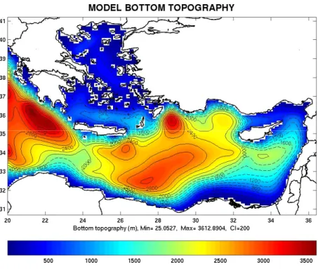
tal diffusion terms are evaluated using the Smagorinsky (1963) diffusion formulation while the vertical mixing coefficients are computed according to the Mellor-Yamada 2.5 turbulence closure scheme (Mellor and Yamada, 1982). The model has one open boundary located at 20◦E as shown in Fig. 1 where open boundary conditions apply. The computational grid has a horizontal resolution of 1/10◦×1/10◦and 25 sigma levels
20
in the vertical with a logarithmic distribution near the sea surface, which results in a better representation of the surface mixed layer. Considering the size (10–14 km) of the internal Rossby radius of deformation for the Eastern Mediterranean basin, such a model resolution (∼5 km) can marginally resolve the mesoscale eddy activity. The U.S. Navy Digital Bathymetric Data Base 5 (1/12◦×1/12◦) was used for building up
25
the model’s bathymetry using bilinear interpolation to map the data onto the model’s grid. The model is very similar to the ALERMO model used in Korres and Lascaratos
OSD
3, 1569–1608, 2006Data assimilation into Eastern Mediterranean Ecosystem Model G. Triantafyllou et al. Title Page Abstract Introduction Conclusions References Tables Figures J I J I Back Close
Full Screen / Esc
Printer-friendly Version
Interactive Discussion (2003) with the only exception being the horizontal resolution (coarser) as the
compu-tational burden in this particular study was very high due to coupling with the BFM, the incorporation of data assimilation and the execution of several sensitivity tests. The model includes parameterization of the Dardanelles net outflow into the Aegean Sea, the runoff of the major rivers of the Thermaikos Gulf (Aliakmonas, Axios and Loudias)
5
and the runoff of Nestos and Evros rivers to north-central and north-eastern Greece. The Dardanelles outflow into the Aegean Sea is a dominant factor for the freshwater budget of the basin, providing approximately 300 km3 of brackish water on an annual basis. The main Greek rivers (Axios, Aliakmonas, Gallikos, Pinios, Sperchios, Evros, Strimonas and Nestos) on the other hand, with a total runoff of ∼19 km3/yr, have a
10
much lower contribution. Even lower is the contribution of the Turkish rivers with a total runoff of ∼5 km3/yr.
2.2 Biochemical Flux Model
BFM is a generic highly complex model based on the European Regional Seas Ecosys-tem Model (ERSEM) (Baretta et al., 1995; Vichi et al., 2004). Although a detailed
15
description of the BFM and its implementation in the Eastern Mediterranean can be found in a companion paper Petihakis et al. (2006), a brief presentation is considered necessary for those not familiar with the particular model. As in ERSEM the model uses a functional group approach separating the organisms according to their trophic level (producers, consumers and decomposers) and further subdivided on the basis of
20
their trophic links and/or size. Although within each trophic level the groups have the same processes, differentiation is achieved through the different parameter values. All the important physiological (ingestion, respiration, excretion and egestion), and pop-ulation (growth, migration and mortality) processes are included, and are described by fluxes of carbon and nutrients. Carbon is the basic unit cycled in the system,
fol-25
lowed by macronutrients, chlorophyll and oxygen, with variable carbon/nutrients and carbon/chl-a ratios. Following the model’s food web, diatoms are preyed on by mi-crozooplankton and omnivorous mesozooplankton, nano-phytoplankton to an extent
OSD
3, 1569–1608, 2006Data assimilation into Eastern Mediterranean Ecosystem Model G. Triantafyllou et al. Title Page Abstract Introduction Conclusions References Tables Figures J I J I Back Close
Full Screen / Esc
Printer-friendly Version
Interactive Discussion by heterotrophic nanoflagellates but mostly by microzooplankton, pico-phytoplankton
mostly by heterotrophic nanofalgellates and to a lesser extent by microzooplankton and finally large phytoplankton by microzooplankton and omnivorous mesozooplankton. Bacteria consume Dissolved Organic Carbon (DOC) both labile and semi-labile, act as decomposers on Particulate Organic Carbon (POC) and compete with phytoplankton
5
for inorganic nutrients. Their main predators are the heterotrophic nanoflagellates while a small part is also channelled to microzooplankton. Heterotrophic nanoflagellates are preyed on by microzooplankton which in turn is eaten by omnivorous mesozooplankton. Omnivorous mesozooplankton is preyed on by carnivorous mesozooplankton which is the top predator of the food chain. For all consumers there is feeding within the same
10
functional group (cannibalism), which acts as a stabilizing mechanism. 2.3 Climatological run
The model’s climatological run was initialized with the Mediterranean Ocean Data-Base (MODB-MED4) (Brasseur et al., 1996) which contains seasonal profiles of temperature and salinity mapped on a 1/4◦×1/4◦ horizontal grid. These data were mapped onto
15
the model’s horizontal grid using bilinear interpolation. Additionally, initial velocities were set to zero. The temperature and salinity profiles at the Eastern open boundary were also derived from the same database. The integration starts with spring initial conditions (15 May), although sensitivity tests have shown that the starting season of the integration does not play a crucial role in determining the results. The model
20
is integrated using a “perpetual year” forcing atmospheric data set. More specifically the momentum surface budget was specified according to the ECMWF wind stress monthly climatology (Korres and Lascaratos, 2003). Finally, the heat flux and water flux boundary conditions at the surface were set as follows:
ρocpKH ∂ T ∂ z z=0 =QT − QSOL+ c1(T∗− T1) (1) 25 1576
OSD
3, 1569–1608, 2006Data assimilation into Eastern Mediterranean Ecosystem Model G. Triantafyllou et al. Title Page Abstract Introduction Conclusions References Tables Figures J I J I Back Close
Full Screen / Esc
Printer-friendly Version Interactive Discussion wσ = 0 = E−P −R +c2S ∗−S 1 S1 (2)
where QT is the monthly average total heat flux field, E is the evaporation rate taken from the Kondo-Bignami monthly climatology, precipitation rate P is taken from Jaeger’s monthly climatology and T∗, S∗fields are taken from MODB-MED4 SST and SSS sea-sonal climatology. Solar radiation flux QSOL is calculated with the Reed formula using
5
the ECMWF monthly cloud cover data. The initial conditions for the nutrients are taken from Levitus (1982) while the other biochemical state variables from the 3-D ecosys-tem model for the Cretan Sea (Petihakis et al., 2002). The model was run perpetually for four years in order to reach a quasi steady state and to obtain inner fields fully co-herent with the boundary conditions. The ecosystem pelagic state variables along the
10
open boundary are described by solving water column 1-D ecosystem models at each surface grid point on the open boundary.
2.4 Hindcast experiment
In this experiment the model was integrated for a period of one year (January 1999– December 1999) and initialized from the climatological run. At the same time the model
15
was asynchronously coupled with the coarse resolution (0.5◦×0.5◦) ECMWF 6 hour at-mospheric data (wind velocity, air temperature, relative humidity and cloud cover) for the same period covering the whole Mediterranean basin. This set of atmospheric data was used by the air-sea interaction scheme of the model for the estimation of heat, freshwater and momentum fluxes at the sea surface. In order to adjust the basin
20
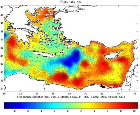
climatological dynamics to the interannual forcing, the model was integrated twice us-ing the same atmospheric data set. The free surface elevation distribution for the 1st Jan 1999 (during the second year of model integration) is shown in Fig. 2 where an intense and elongated Rhodes gyre with a strong Mersha Matruh anticylconic gyre to its southern boundary are depicted.
25
OSD
3, 1569–1608, 2006Data assimilation into Eastern Mediterranean Ecosystem Model G. Triantafyllou et al. Title Page Abstract Introduction Conclusions References Tables Figures J I J I Back Close
Full Screen / Esc
Printer-friendly Version
Interactive Discussion
3 Ocean color data
Daily data from the SeaWiFS sensor onboard the SeaStar satellite at local area cov-erage spatial resolution (∼1.1 km by 1.1 km pixels) for one year (1999) were used for this study. This represented more than 20 GB of data which were acquired from NASA Goddard through the NASA Ocean Colour Web and ftp service (Feldman and
Mc-5
Clain, 2004). The data were processed by the NASA SeaDAS software v4.0 (Baith et al., 2001) from the original spectral data using default values from the SeaWiFS level 2 product processing chain which includes atmospheric correction, georeferenc-ing and chlorophyll-a retrieval OC4v4 (O’Reilly et al., 2000; Patt et al., 2003). The OC4v4 algorithm implements the following fourth order polynomial equation to
calcu-10
late chlorophyll-a estimates
log10(chl − a)=0.366 − 3.067R4S+ 1.930R4S2 + 0.649R4S3 − 1.532R4
4S (3)
where R is reflectance, R4S is the maximum value of R443/R555, R490/R555or R510/R555 and 443, 490, 510 and 555 represent the wavelengths of the four SeaWiFS bands used. The OC4v4 algorithm was designed for biological studies of the global oceanic
15
environment. This empirical method of estimating chlorophyll-a has been found to give reasonably accurate estimates for most case-I waters (Bricaud et al., 2002), overes-timate concentrations under certain oligotrophic conditions for case-I waters and be inaccurate for case-II waters of the Eastern Mediterranean (Bricaud et al., 2002; San-cak et al., 2005). However, at the time of processing and data assimilation, for the
20
year under investigation, these SeaWiFS data were the best available satellite derived a concentration estimates for the area of interest. The daily chlorophyll-a estimchlorophyll-ates were remchlorophyll-apped to chlorophyll-a flchlorophyll-at grid using chlorophyll-a cylindricchlorophyll-al equidistchlorophyll-ant projection, again using the NASA SeaDAS software. Finally, weekly (8 day) averages were pro-duced that took into account a land mask and data masked by clouds, and provided
25
girdded chlorophyll estimates suitable for assimilation into the coupled hydrodynamic-ecosystem models.
OSD
3, 1569–1608, 2006Data assimilation into Eastern Mediterranean Ecosystem Model G. Triantafyllou et al. Title Page Abstract Introduction Conclusions References Tables Figures J I J I Back Close
Full Screen / Esc
Printer-friendly Version
Interactive Discussion
4 The assimilation scheme
The assimilation scheme is sequential and is based on the Singular Evolutive Extended Kalman (SEEK) filter developed by Pham et al. (1997). The SEEK filter is a simplified Extended Kalman (EK) filter suitable for applications with high dimensional systems (the system dimension is denoted by N), as in meteorology and oceanography. The
5
filter avoids the prohibitive computational burden associated to the significant size of the EK filter N × N-error covariance matrices (denoted by P ) by operating with low-rank error covariance matrices. More precisely, the SEEK filter uses the classical decom-position P=LULT of a low-rank matrix, where L and U are and r×r matrices, so that numerical calculations involving P can be likewise achieved by means of L and U .
10
This allows drastic computational savings in time and storage without requiring major changes in the EK filter’s algorithm. Starting from an initial low-rank r error covariance matrix obtained via an Empirical Orthogonal Functions (EOF) analysis (see below), Pham et al. (1997) showed that when the model dynamics are perfect (no model er-ror), the EK filter error covariance matrices always remain of the same rank r. The EK
15
filter analysis step is then only applied along the directions of L; hence its columns will be called the correction directions of the filter. When the model is imperfect, the model error can be projected onto the subspace spanned by the correction direction to avoid continuous increase in the rank of the error covariance matrices. In its most general form, the correction directions of the SEEK filter evolves its correction directions in time
20
with the tangent linear model to follow changes in the model dynamics. In this study, however, these directions were kept invariant for reasons explained below. The filter’s algorithm is summarized below. A more detailed description can be found in Pham et al. (1997).
4.1 The filter algorithm
25
Consider the system state vector Xkt to be partly observed only at specific times tk, between times t1 and tend. The state vector is assumed to advance from time tk to
OSD
3, 1569–1608, 2006Data assimilation into Eastern Mediterranean Ecosystem Model G. Triantafyllou et al. Title Page Abstract Introduction Conclusions References Tables Figures J I J I Back Close
Full Screen / Esc
Printer-friendly Version
Interactive Discussion time tk+1according to the forecast model
Xkt+1=Mk,k+1(Xkt)+ηk+1 (4)
where M is the transition operator, representing the model dynamics, and η is a white noise process, describing the model error, with zero mean and covariance matrixQ. A
vector of observations Yko at time tk, function of the system state Xkt and a
measure-5
ment of uncertainty
Yko=Hk(Xkt)+ εk (5)
is assumed to be available. Hk is the observation operator and εk is the error in the observations, which will be assumed white with known spatial covariance matrix R.
These observations are entrained serially with the forecast state Xkf to produce the
10
analysis state Xka as
Xka=Xkf + Gk[Yko− HkXkf] (6)
in which the matrix G is referred to as the gain matrix of the filter. The forecast is
obtained by advancing the previous analyzed state Xkawith the forecast model
Xkf + 1=Mk,k+1(Xka). (7)
15
The gain matrixG interpolates between the observations and the forecast. The (sub-)
optimal gain G of the EK filter can be obtained by formulating a variational problem to find the gain that minimizes the expected error between the analysis state and the true state (Jazwinski, 1970). The optimality of the Kalman gain is predicated on the knowledge of the forecast error covariance matrixPf. At time tk, it is given by
20
Gk=PkfHtk[HkPkfHTk+R]−1, (8)
whereHk denotes the linearization of the observation operator Hk about the forecast state Xkf. The analysis tends to adapt the forecast or the observations according to their
OSD
3, 1569–1608, 2006Data assimilation into Eastern Mediterranean Ecosystem Model G. Triantafyllou et al. Title Page Abstract Introduction Conclusions References Tables Figures J I J I Back Close
Full Screen / Esc
Printer-friendly Version
Interactive Discussion respective predicted uncertainties HKPkfHTk and R. Alternatively, when the forecast
error covariance matrix is decomposed as Pkf=LkUk−1LTk as in the SEEK filter, the Kalman gain can be computed from
Gk=LkUk(HkLk)T (9)
in which the matrixU is updated according to
5 Uk−1=[Uk−1+ PLT kQPLk] −1+ (H kLk)TR−1HkLk, (10) and PL k=(L T kLk) −1
Lk is the projection operator onto the subspace spanned by the columns of Lk. This shows that the analyzed state is a linear combination of the cor-rection dicor-rections.
The extent to which the forecast is adopted depends on the analysis error covariance
10
matrix Pa, which is first obtained as a correction of the forecast error covariance matrix using the observation statistics
Pka= Pkf − GkHkPkf = LkUkLTk (11)
and then advanced in time according to the model dynamics to produce the next fore-cast error covariance matrix
15
Pkf+1=Mk,k+1PkaMk,kT +1+ Q=Lk+1UkLk+1+ Q, (12) where the new correction directions Lk+1 evolve in time with the tangent linear model
Mk,k+1(evaluated about the analyzed state Xka) according to
Lk+1=Mk,k+1Lk. (13)
It is important to realize that Eqs. (11) and (12), expressing the analysis and forecast
20
error covariance matrices, are not needed for the filters’ algorithms. They have only been included for completeness. The evolution of the correction directions is generally beneficial to keep track of changes in the model dynamics (Hoteit et al., 2002; Hoteit
OSD
3, 1569–1608, 2006Data assimilation into Eastern Mediterranean Ecosystem Model G. Triantafyllou et al. Title Page Abstract Introduction Conclusions References Tables Figures J I J I Back Close
Full Screen / Esc
Printer-friendly Version
Interactive Discussion and Pham, 2003). The numerical integration of Eq. (3) requires, however, r+1 times
forecast model runs, which can be rather significant with a heavily loaded coupled physical-biochemical model such as the one used in this study. Following Brasseur et al. (1999), who found that a reliable set of invariant EOFs may provide a good correc-tion subspace for quasi-linear dynamical models, the correccorrec-tion direccorrec-tions of the SEEK
5
filter were kept invariant in the present study. Theoretically, this can be supported by assuming that the ecosystem state generally undergoes little change between two con-secutive observations, which allows considering forMk,k+1 to be equal to the identity matrix. In practice, several studies (e.g. Carmillet et al., 2001; Hoteit et al., 2003), suggested that performance losses associated with this approximation were not
sig-10
nificant given the achieved drastic reduction in the computational burden of the SEEK filter. Indeed, only one model integration is now required to compute the forecast state while the filter error covariance matrices are parameterized by means of a set of EOFs describing the dominant modes of the system’s variability.
4.2 Localization of the filter analysis
15
The low-rank approximation generally results in very few degrees of freedom for the fil-ter analysis to fit available observations. Another difficulty in the assimilation system is that the initial EOFs correction directions are not updated with model dynamics. These functions, especially those associated with the least energetic modes, can be spoiled with spurious auto/cross correlations, which inevitably introduces noise into the filter
20
analysis. As suggested by Houtekamer and Mitchel (2001), a simple strategy to deal with this problem is to exclude observations greatly distant from the grid point being analyzed. This allows the retention of the structures of the short-range correlations in the filter’s error covariance matrices, which are assumed to be more reliable, while filtering out long-range correlations. This “localization” of the filter analysis can be e
ffi-25
ciently implemented through a Schur product (an element by element multiplication) of the error covariance matrix and a correlation function with local support (Gaspari and
OSD
3, 1569–1608, 2006Data assimilation into Eastern Mediterranean Ecosystem Model G. Triantafyllou et al. Title Page Abstract Introduction Conclusions References Tables Figures J I J I Back Close
Full Screen / Esc
Printer-friendly Version
Interactive Discussion Cohn, 1999). In this approach, the filter’s gain in Eq. (8) is reformulated as
Gk = (γ ◦ PkT)HTk[Hk(γ ◦ Pkf)HTk+ R]−1, (14) where γ ◦ Pkf denotes the Schur product of the forecast covariance matrix Pkf with the localization function γ. Although this formulation entails an approximation in the filter’s algorithm, it is naturally supported by the fact that only data points located in
5
the “neighbourhood” of an analyzed grid point should contribute to the analysis at this point.
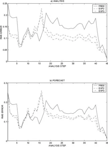
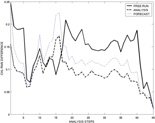
In the current system, the localization function is defined by means of a radius of in-fluence d (in km) around the analyzed grid point. All data located outside this horizontal (× 24 vertical levels) area of influence are not retained in the analysis. Assimilation
ex-10
periments were performed in order to find an appropriate value for d. Figure 3 shows the time evolution of the Chl-a Root Mean Square (RMS) estimation error (data/model misfit) for the forecast (i.e. just before the assimilation of the new observations) and the analysis as they result from three assimilation runs with different choices of the radius of influence: 150 km (EXP3), 70 km (EXP4) and 250 km (EXP5), respectively. RMS of
15
the model free-run (i.e. model run without assimilation) is also shown. The assimilation system behaves poorly with d=70 km. Although the choice of 250 km seems to be the best in terms of the analysis RMS error; the forecast system shows some weakness with such a large choice of d, as can be noticed from the forecast RMS during the period of spring bloom between March and April. This significant increase in the
fore-20
cast RMS during this period of model regime change is probably due to some spurious large-range correlations represented in the EOFs correction directions, and therefore in the filter analyses, which the model was not able to properly assimilate. These re-sults suggest that a radius of influence should be chosen neither too large to filter out spurious large-range correlations, nor too small in order to obtain a smooth analysis
25
state. Given these conclusions, a radius of influence d=150 km was therefore selected in the sequel.
OSD
3, 1569–1608, 2006Data assimilation into Eastern Mediterranean Ecosystem Model G. Triantafyllou et al. Title Page Abstract Introduction Conclusions References Tables Figures J I J I Back Close
Full Screen / Esc
Printer-friendly Version
Interactive Discussion 4.3 Model and observational errors
The observational and model error covariance matricesR and Q need to be specified
in the filter’s algorithm. These matrices are generally very poorly known. It is common to consider a diagonal observation error covariance matrix R, which means that the
observations are assumed to be spatially uncorrelated, but this can be partly accounted
5
for by overestimating the diagonal coefficients of R, which were set as a fraction of the variance of the satellite observations at each grid point. The specification ofQ is
considerably more complex because very little information is available about the model error, and because of the significant number (N×N) of parameters that need to be estimated. Following Pham et al. (1997), a compensation technique is used to replace
10
the term PLT
kQkPLk in Eq. (10) by a forgetting factor ρ which artificially amplifies the background error covariance matrix. This leads to a new update formula for the matrix
U:
Uk−1=1/ρUk−1−1+ (HkLk)TRk−1HkLk (15)
The value of ρ depends on the system under study, as it can be further used to account
15
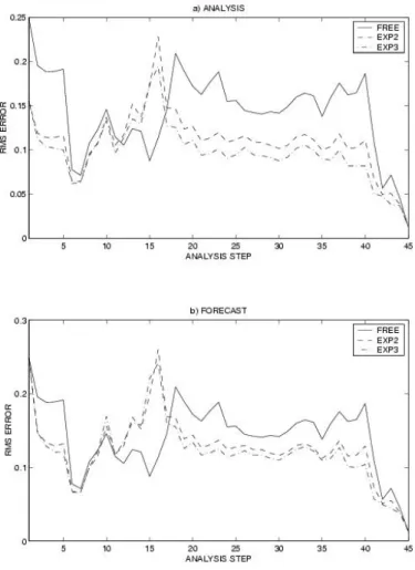
for other sources of errors in the filter, such as the underestimation of the error covari-ance matrices by low-rank matrices or the linearization errors, by giving more weight to recent observations. ρ was empirically set to 0.3 after several sensitivity assimilation experiments with different values of ρ ranging between 0.1 and 0.9. As an example, in Fig. 4 the RMS error for two experiments with different choices of ρ (EXP2: 0.6; EXP3:
20
0.3) is shown. Overall, in terms of both the analysis and the forecast RMS error, the choice of 0.3 seems to be the most appropriate.
4.4 The correction directions
A common strategy to determine the filter’s correction directions is to use model statis-tics as an approximation of the true system statisstatis-tics (Pham et al., 1997). Then by
25
appropriate sampling of model state vectors one can obtain an approximation of the fil-1584
OSD
3, 1569–1608, 2006Data assimilation into Eastern Mediterranean Ecosystem Model G. Triantafyllou et al. Title Page Abstract Introduction Conclusions References Tables Figures J I J I Back Close
Full Screen / Esc
Printer-friendly Version
Interactive Discussion ter’s covariance matrix through the dominant empirical orthogonal functions (EOFs). In
the twin experiments setup (not presented here), the physical model was first integrated for a 4-year period in order to achieve a quasi adjustment of the model climatological dynamics. Next, another integration of 4 years of the coupled system (physical & bio-chemical model) was carried out to generate a historical sequence of model states,
5
sampled every 2 days during the last two years of the integration. Since the state vari-ables are of different nature, a multivariate EOF analysis was applied to the sampled set of 360 state vectors. In this analysis, model state variables were normalized by the inverse of the square-root of their domain-averaged variances. In the real observations assimilation experiment, the coupled system was initialized with climatology and
inte-10
grated for two years forced with the ECMWF 1999 6 hour data (applied twice). During the last year of integration model, states were sampled and stored every two days in order to calculate the EOFs. For this experiment 25 EOFs were retained explaining 95% of the ecosystem variability.
5 Assimilation of satellite ocean color data for the period 1999
15
This section presents and discusses the results of the main assimilation experiments in which the 1999 SeaWiFS data were assimilated into the Eastern Mediterranean ecosystem model using the SEEK filter with a radius of influence d=150 km and a forgetting factor ρ=0.3. Morel (1998) proposed that the depth sensed by SeaWiFS depends upon the concentration of chlorophyll and the wave band; and for waters
20
with chlorophyll ≤0.1 mg/m3, as in the case of the Levantine, this depth is about 30 m. In this study the observation operator Hk integrates vertically the model calculated chlorophyll profiles for the four phytoplankton groups over the first 30 m in the relevant filter equations.
We first analyze the overall behavior of the assimilation system then we study the
25
impact of the assimilation of ocean colour data on the other ecological components of the model. This will allow us to assess (i) the relevance of the assimilation scheme
OSD
3, 1569–1608, 2006Data assimilation into Eastern Mediterranean Ecosystem Model G. Triantafyllou et al. Title Page Abstract Introduction Conclusions References Tables Figures J I J I Back Close
Full Screen / Esc
Printer-friendly Version
Interactive Discussion to efficiently propagate these surface observations into the deep ocean, and (ii) the
ability of the BFM model to properly assimilate the information from the SeaWiFS data. Figure 5 plots the time evolution of the RMS misfit between the assimilated chlorophyll data and the estimated chlorophyll concentrations as it results from the model free-run (without assimilation), and the filter run before (forecast) and after (analysis) the filter’s
5
correction. Overall the filter’s behavior is quite satisfactory and obviously improves the model/data consistency. The RMS error for both the forecast and the analysis is al-ways smaller than the RMS error of the free-run except for the period of spring bloom between the end of March and the end of April, where the filter, particularly the fore-cast state, was not able to follow the rapid changes in the ecosystem state. The poor
10
behavior of the filter during this period is probably due to the misrepresentation of the bloom event in the EOFs based correction directions. The use of seasonal sets of EOFs associated with the major ecological events, and the evolution of the correction directions with the model dynamics can be expected to improve the behavior of the filter during this period. The filter correction step efficiently improves the forecast after every
15
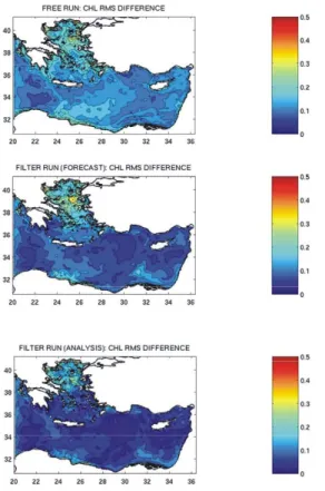
filtering cycle suggesting the importance of the data assimilation into the model. The resulting analysis state is also shown to respect the dynamic balance in the model, as the forecast RMS error remains stable over time, allowing the BFM model to properly assimilate the SeaWiFS data. The spatial distribution for the chlorophyll RMS model-filter/data differences averaged over the entire assimilation window is shown in Fig. 6.
20
As expected, the model free-run/data differences are the largest, with the worst model performance observed in the northern Aegean Sea between Greece and Turkey and close to the northern coast of Africa. The filter forecast RMS error is better than that of the free-run over the whole Eastern Mediterranean except in the northern Aegean Sea region where the model error is significant. The RMS estimation error is
signif-25
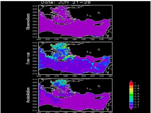
icantly reduced over the whole domain after the filter analysis is applied. Figure 7 shows chlorophyll concentrations at the surface from satellite observations (top panel), model free-run (central panel) and analysis (lower panel) for the period 21 to 28 June. Following Morel (1998) in order to compare satellite observations with model results,
OSD
3, 1569–1608, 2006Data assimilation into Eastern Mediterranean Ecosystem Model G. Triantafyllou et al. Title Page Abstract Introduction Conclusions References Tables Figures J I J I Back Close
Full Screen / Esc
Printer-friendly Version
Interactive Discussion surface chlorophyll concentrations produced by the model were integrated over 30 m
depth and averaged over the same period. The model free run significantly overesti-mates the surface chlorophyll concentrations in the Levantine Sea and particularly in the Aegean Sea. The filter successfully corrects the forecast particularly over the Lev-antine Sea. However, the filter’s improvement over the Aegean Sea is not significant;
5
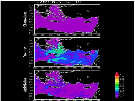
and the filter was unable to completely follow the rapid increase in the chlorophyll con-centrations over this area. Figure 8 shows the same fields as Fig. 7 but for the period 12–19 November. The model free-run overestimates the chlorophyll concentrations in the Levantine and south the Aegean Sea. As it is shown (lower panel) the filter per-forms efficiently driving the model closer to the satellite observations. Figure 9 depicts
10
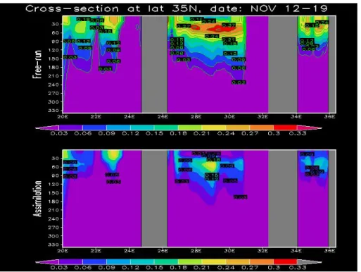
an East–West cross section of the chlorophyll concentrations at 35◦N. A comparison between the free-run and the analysis fields show remarkable differences as the filter effectively propagates the observed information of the low chlorophyll concentrations at surface to the deeper layers. The analysis fields display smaller-scale vertical struc-tures while the concentrations at the deep chlorophyll maximum (DCM) are significantly
15
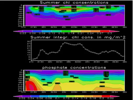
lower. Specifically, the DCM concentrations have decreased from 0.37 to 0.22 mg/m3in the area of the Rhodes gyre. To further assess the ecosystem functioning of the assim-ilation system in the deep layers, Fig. 10 plots a North–South cross section of different ecological variables at longitude 28.5◦E (area of the Rhodes Gyre) during the summer period as they result from the assimilation system. Knowledge about the biochemical
20
processes in this area that has been extensively studied by Krom et al. (2003) can be used to validate the behavior of the assimilation system. The Rhodes Gyre is a cold core eddy that tends to change intensity, size and location with time. The main char-acteristic of the Gyre is the upwelling of nutrients in the center that results in increased phytoplankton biomass and primary productivity. The top panel shows the vertical
dis-25
tribution of the chlorophyll concentrations where the DCM is depicted at 60 m with a magnitude of ∼0.3 mg/m3in close agreement with Salihoglu et al. (1990). The middle panel shows the integrated chlorophyll. The peak has a magnitude of ∼28 mg/m2which is a slight underestimation compared to 39 mg/m2as estimated by Ediger and Yilmaz
OSD
3, 1569–1608, 2006Data assimilation into Eastern Mediterranean Ecosystem Model G. Triantafyllou et al. Title Page Abstract Introduction Conclusions References Tables Figures J I J I Back Close
Full Screen / Esc
Printer-friendly Version
Interactive Discussion (1996). The phosphate concentrations plotted in the lower panel shows a formation
of nutricline at 75 m. Phosphorous has been depleted in the upper layers exhibiting concentration values less than 0.02 µg-at/l, while in cross section phosphate increases with depth to a maximum of 0.22 µ g-at/l.
The impact of assimilating ocean colour data into the BFM model dynamics is also
5
assessed in Fig. 11 which plots the time evolution of the depth integrated chl-a con-centrations for the Rhodes gyre as it results from the model free-run and as estimated by the assimilation system. The model free-run without any assimilation provides quite good estimates of the integrated chl-a concentrations (35 mg/m2) compared to the ones produced by the field measurements (39 mg/m2). The assimilation of ocean colour data
10
clearly reduces the surface chl-a concentrations pushing the model top layers towards a more oligothrophic condition according to the information extracted from the obser-vations. However this drives the system dynamics away from the “truth” in the deep layers, not-visible by the satellite, subsequently reducing the depth integrated chl-a concentrations, being in disagreement with the observed values. This demonstrates
15
the limitations of assimilating only surface ocean colour data and calls for the need of constraining the model dynamics with subsurface ecological data as well.
Having stated the above limitation of the current assimilation system in oligotrophic areas, which is mainly related to complex ecological processes associated with cy-clonic gyres and upwelling areas, the overall performance of the assimilation is in
gen-20
eral very positive as can be, for example, seen in the spatially integrated chl-a con-centration during August (Fig. 12). The values resulting from the assimilation system are quite closer to the measured concentrations of Ignatiades et al. (2002); Siokou-Frangou et al. (2002) than those simulated by the model free-run. Looking at the decomposers plots shown in Fig. 13, both the model free-run and the assimilation run
25
are within the range of measured values in the North, North-East and South Aegean. The free run exhibits a more uniform spatial pattern, in contrast to the one estimated by the assimilation system which exhibits significantly more spatial variability. Bacteria in oligotrophic systems play a very important role as they remineralise and consume
OSD
3, 1569–1608, 2006Data assimilation into Eastern Mediterranean Ecosystem Model G. Triantafyllou et al. Title Page Abstract Introduction Conclusions References Tables Figures J I J I Back Close
Full Screen / Esc
Printer-friendly Version
Interactive Discussion trients (which are in short supply), sustaining an active microbial loop. As their growth
depends on the available nutrient concentrations, which in turn are strongly coupled to the hydrodynamic fields, one would expect such strong spatial variability to be in agree-ment with the characteristics of the complex system of gyres and jets of the Eastern Mediterranean.
5
6 Conclusions
This study describes the implementation of an advanced marine ecosystem asilation system based on a complex three-dimensional ecological model and a sim-plified Extended Kalman filter to assimilate SeaWiFS ocean colour data in the East-ern Mediterranean. The model is composed of two coupled sub-models: the
physi-10
cal Princeton Ocean model (POM) and the Biochemical Flux Model (BFM). The filter is based on the Singular Evolutive Extended Kalman (SEEK) filter, in which the er-ror statistics were parameterized by means of a suitable set of Empirical Orthogonal Functions (EOFs). A localization of the filter analysis step was implemented to filter out any spurious long-range correlations in the EOFs. After several sensitivity experiments
15
which were performed in order to find the best values for some of the filter parameters, a hindcast experiment was conducted for the year 1999 with the aim of demonstrating the effectiveness of this system and, at the same time, to assess the relevance of its outputs. The results of this main experiment clearly demonstrate that the assimilation system operates in a satisfactory way; the system was capable of efficiently fitting the
20
assimilated data, and the filter efficiently propagated the surface observations to the deep layers. Furthermore, the assimilation significantly improves the model behaviour and the impact of the satellite ocean colour data on all the model’s ecological com-ponents was mainly positive. This is in agreement with the multivariate character of the filter’s correction directions which retain the cross correlations existing between the
25
different model variables. These positive results do not mean that the system is per-fect as some weaknesses were observed especially in the complex oligotrophic areas;
OSD
3, 1569–1608, 2006Data assimilation into Eastern Mediterranean Ecosystem Model G. Triantafyllou et al. Title Page Abstract Introduction Conclusions References Tables Figures J I J I Back Close
Full Screen / Esc
Printer-friendly Version
Interactive Discussion adjustments having been made in order to improve the model/data consistency, the
filter nevertheless did not adjust several ecological components in the deep layers well enough to cover significant model errors not represented in the assimilation system. In practice, any model of the real ecosystem will have important deficiencies that cannot be easily estimated because of the large dimension of the system and a serious dearth
5
of observations, especially in the deep layers. Even though the availability of a limited subsurface data set might not be enough to solve this problem, the assimilation of these data would constrain the model variability in the deep layers and help to prevent any deviation from reality. Another important issue related to this problem is the assumption of “perfect physics” considered in this study. The improvement of the physical solution
10
through the assimilation of physical data is expected to significantly improve the be-havior of the coupled model, resulting in fewer model errors in the ecological solution. The quality of the data was also an issue in the present study. One solution could be to assimilate the colour data directly, rather than converting it to chlorophyll, by including a bio-optical algorithm to predict the colour from the model phytoplankton values, which
15
may result in a reduction of the uncertainties in the data. Despite the use of a state-of-the-art coupled physical-biochemical marine ecosystem model constrained with the most synoptic ecological data sets using an advanced Kalman filter based assimilation scheme, the overall results of this study are still at a preliminary stage, though giving all the improvements that can be reported to the system. This study, however, clearly
20
indicates that the development of an assimilation system providing reliable estimates of the ecosystem state is achievable, and this is true not only for the Eastern Mediter-ranean, but for any area of the global ocean. This conclusion is of particular interest for the marine ecosystem community and provides us with encouraging and promising results for future developments.
25
Acknowledgements. This work was supported by the Mediterranean Forecasting System –
To-wards Environmental Predictions Project (MFSTEP). Contract no. EVK3-CT-2002-00075 NASA Goddard Distributed Active Archive Centre is gratefully acknowledged for the supply of the Sea-WiFS data.
OSD
3, 1569–1608, 2006Data assimilation into Eastern Mediterranean Ecosystem Model G. Triantafyllou et al. Title Page Abstract Introduction Conclusions References Tables Figures J I J I Back Close
Full Screen / Esc
Printer-friendly Version
Interactive Discussion References
Allen, J. I., Ekenes, M., and Evensen, G.: An Ensemble Kalman Filter with a complex marine ecosystem model: Hindcasting phytoplankton in the Cretan Sea, Ann. Geophys., 21, 399– 411, 2002.
Anderson, L. A., Robinson, A. R., and Lozano, C. J.: Physical and biological modeling in the
5
Gulf Stream region: Data assimilation methodology, Deep Sea Res., 47, 1787–1827, 2000. Baith, K., Lindsay, R., Fu, G., and McClain, C. R.: SeaDAS, A Data Analysis System for
Ocean-Color Satellite Sensors, EOS Trans. AGU, pp. 202, 2001.
Baretta, J. W., Ebenhoh, W., and Ruardij, P.: The European Regional Seas Ecosystem Model, a complex marine ecosystem model, Netherlands Journal of Sea Research, 33, 233–246,
10
1995.
Blumberg, A. F. and Mellor, G. L.: Diagnostic and prognostic numerical circulation studies of the South Atlantic Bight, J. Geophys. Res., 88, 4579–4592, 1983.
Blumberg, A. F. and Mellor, G. L.: A description of a three-dimensional coastal ocean circulation model, in: Three-Dimensional Coastal Ocean Circulation Models, edited by: Heaps, N. S.,
15
Coastal Estuarine Science, AGU, Washington, D.C., pp. 1–16, 1987.
Brasseur, P., Ballabrera-Poy, J., and Verron, J.: Assimilation of altimetric observations in a primitive equation model of the Gulf Stream using a singular evolutive extended Kalman filter, J. Mar. Syst., 22(4), 269–294, 1999.
Brasseur, P., Brankart, J.-M., Schoenauen, R., and Beckers, J.-M.: Seasonal Temperature and
20
Salinity Fields in the Mediterranean Sea, Climatological Analyses of an Historical Data Set, Deep Sea Res., 43, 159–192, 1996.
Bricaud, A., Bosc, E., and Antoine, D.: Algal Biomass and Sea Surface Temperature in the Mediterranean Basin. Intercomparison of Data from Various Satellite Sensors, and Implica-tions for Primary Production Estimates, Remote Sens. Environ., 81, 163–178, 2002.
25
Cane, M. A., Kaplan, A., Miller, R. N., et al.: Mapping tropical Pacific sea level: data assimilation via a reduced state Kalman filter, J. Geophys. Res., 101(C10), 22 599–22 617, 1996. Carmillet, V., Brankart, J. M., Brasseur, P., et al.: A singular evolutive extended Kalman filter
to assimilate ocean color data in a coupled physical-biochemical model of the North Atlantic ocean, Ocean Modelling, 3(3–4), 167–192, 2001.
30
Drakopoulos, P. G. and Lascaratos, A.: Modelling the Mediterranean Sea, climatological forc-ing, J. Mar. Syst., 20, 157–173, 1997.
OSD
3, 1569–1608, 2006Data assimilation into Eastern Mediterranean Ecosystem Model G. Triantafyllou et al. Title Page Abstract Introduction Conclusions References Tables Figures J I J I Back Close
Full Screen / Esc
Printer-friendly Version
Interactive Discussion Ediger, D. and Yilmaz, A.: Characteristics of deep chlorophill maximum in the Northeastern
Mediterranean with respect to environmental conditions, J. Mar. Syst., 9, 291–303, 1996. Fasham, M. J. R. and Evans, G. T.: The use of optimization techniques to model marine
ecosys-tem dynamics at the JGOFS station at 47 N 20 W., Trans. R. Soc. Lond., Ser. B, 348, 203– 209, 1995.
5
Feldman, G. C. and McClain, C. R.: Ocean Color Web, SeaWiFS Reprocessing, 4, 2004. Fennel, K., Losch, M., Schroter, J., and Wenzel, M.: Testing a marine ecosystem model:
sen-sitivity analysis and parameter optimization, J. Mar. Syst., 28, 45–63, 2001.
Friedrichs, M. A. M.: Assimilation of JGOFS EqPac and SeaWiFS data into a marine ecosystem model of the Central Equatorial Pacific Ocean, Deep-Sea Res. II, 49(1–3), 289–319, 2001.
10
Fukumori, I. and Malanotte-Rizzoli, P.: An approximate Kalman filter for ocean data assimila-tion: an example with an idealized Gulf Stream model, J. Geophys. Res., 100(C4), 6777– 6793, 1995.
Gaspari, G. and Cohn, S. E.: Construction of correlation functions in two and three dimensions, Quart. Roy. Meteorol. Soc., 125, 723–757, 1999.
15
Ghil, M. and Malanotte-Rizzoli, P.: Data assimilation in meteorology and oceanography, Adv. Geophys., 33, 141–266, 1991.
Gunson, J., Oschlies, A., and Garcon, V.: Sensitivity of ecosystem parameters to simulated satellite ocean color data using a coupled physical-biological model of the North Atlantic, J. Mar. Res., 57, 613–639, 1999.
20
Harmon, R. and Challenor, P.: A Markov chain Monte Carlo method for estimation assimilation into models, Ecological modelling, 101, 41–59, 1996.
Horton, C., Cliford, M., Schmitz, J., and Kantha, L. H.: A real-time oceanographic now-cast/forecast system for the Mediterranean sea, J. Geophys. Res., 102(C11), 25 123–25 156, 1997.
25
Hoteit, I., Pham, D.-T., and Blum, J.: A simplified reduced order kalman filtering and application to altimetric data assimilation in tropical pacific, J. Mar. Syst., 36, 101–127, 2002.
Hoteit, I. and Pham, D. T.: Evolution of the reduced state space and data assimilation schemes ba, sed on the Kalman filter, J. Meteorol. Soc. Japan, 81, 21–39, 2003.
Hoteit, I., Triantafyllou, G., and Petihakis, G.: Towards a data assimilation system for the Cretan
30
Sea ecosystem using a simplified Kalman filter, J. Mar. Syst., 45, 159–171, 2004.
Hoteit, I., Triantafyllou, G., and Petihakis, G.: Efficient Data Assimilation into a Complex 3-D Physical-Biogeochemical Model Using a Semi-Evolutive Partially Local Kalman Filter, Ann.
OSD
3, 1569–1608, 2006Data assimilation into Eastern Mediterranean Ecosystem Model G. Triantafyllou et al. Title Page Abstract Introduction Conclusions References Tables Figures J I J I Back Close
Full Screen / Esc
Printer-friendly Version
Interactive Discussion Geophys., 23, 1–15, 2005.
Hoteit, I., Triantafyllou, G., Petihakis, G., and Allen, J. I.: A singular evolutive extended Kalman filter to assimilate real in situ data in a 1-D marine ecosystem model, Ann. Geophys., 21, 389–397, 2003.
Houtekamer, P. and Mitchel, H.: A sequential ensemble Kalman filter for atmospheric data
5
assimilation, Mon. Wea. Rev., 23, 1–15, 2001.
Ignatiades, L., Psarra, S., Zervakis, V., et al.: Phytoplankton size-based dynamics in the Aegean Sea (Eastern Mediterranean), J. Mar. Syst., 36, 11–28, 2002.
IOCCG: Status and Plans for Satellite Ocean-Colour Missions: Considerations for Complemen-tary Missions, Report No. 2, Dartmouth, Canada, 43 pp., 1999.
10
Jazwinski, A. H.: Stochastic processes and filtering theory, Academic Press, New York, 1970. Korres, G. and Lascaratos, A.: An eddy resolving model for the Aegean and Levantine basins
for the Mediterranean Forecasting System Pilot Project (MFSPP): Implementation and cli-matological runs, Ann. Geophys., 21, 205–220, 2003.
Korres, G. and Lascaratos, A.: An eddy resolving model of the Aegean and Levantine basins
15
for the Mediterranean Forecasting System Pilot Project (MFSPP): Implementation and cli-matological runs, Ann. Geophys., 21, 205–220, 2003.
Krom, M., Groom, S., and Zohary, T.: The Eastern Mediterranean, in: Biogeochemistry of Marine Systems, edited by: Black, K. D. and Shimmield, G. B., Blackwell Publishing, Oxford, pp. 91–126, 2003.
20
Krom, M. D., Brenner, S., Kress, N., Neori, A., and Gordon, L. I.: Nutrient dynamics and new production in a warm-core eddy from the Eastern Mediterranean Sea, Deep-Sea Res., 39(3/4), 467–480, 1992.
Lascaratos, A. and Nittis, K.: A high-resolution three-dimensional study of intermediate water formation in the Levantine Sea, J. Geophys. Res., 103(C9), 18 497–18 511, 1998.
25
Lawson, L. M., Hofmann, E. E., and Spitz, Y. H.: Time series sampling and data assimilation in a very simple ecosystem model, Deep-Sea Res. II, 43(2–3), 625–651, 1996.
Levitus, S.: Climatological Atlas of the World Ocean, NOAA/ERL GFDL, Professional Paper 13, Princeton, N. J., 173pp., 1982.
Matear, R. J.: Parameter optimization and analysis of ecosystem models using simulated
an-30
nealing: A case study at station P., J. Mar. Res., 53, 571–607, 1995.
Mellor, G. L.: User’s guide for a three-dimensional primitive equation, numerical ocean model (July 1998 version), Princeton University, 1998.
OSD
3, 1569–1608, 2006Data assimilation into Eastern Mediterranean Ecosystem Model G. Triantafyllou et al. Title Page Abstract Introduction Conclusions References Tables Figures J I J I Back Close
Full Screen / Esc
Printer-friendly Version
Interactive Discussion Mellor, G. L. and Yamada, T.: Development of a Turbulence Closure Model for Geophysical
Fluid Problems, Rev. Geophys. Space Phys., 20, 851–875, 1982.
Morel, A.: Optical modelling of the upper ocean in relation to its biogenous matter content (case I waters), J. Geophys. Res., 93, 10 749–10 768, 1998.
Natvik, L. J. and Evensen, G.: Assimilation of ocean color data into a biochemical model of the
5
North Atlantic. Part 1., Data assimilation experiments, J. Mar. Syst., 40–41, 155–169, 2002. O’Reilly, J. E., Maritorena, S., O’ Brien, M. C., et al. (Eds.): SeaWiFS Postlaunch Calibration
and Validation Analyses, Part 3, Vol. 11, NASA Goddard Space Flight Centre, Greenbelt, Maryland, 2000.
Patt, F. S., Barnes, R. A., Eplee, R. E. (Jr.), et al.: Algorithm Updates for the Fourth SeaWiFS
10
Data Reprocessing, in: SeaWiFS Postlaunch Technical Report Series, edited by: Hooker, S. B. and Firestone, E. R., NASA Technical Memorandum 32 003–206 892, NASA Goddard Space Flight Centre, Greenbelt, Maryland, 2003.
Petihakis, G., Triantafyllou, G., Allen, J. I., Hoteit, I., and Dounas, C., Modelling the Spatial and Temporal Variability of the Cretan Sea Ecosystem, J. Mar. Syst., 36, 173–196, 2002.
15
Petihakis, G., Triantafyllou, G., Korres, G., Pollani, A., and Hoteit, I.: Eastern Mediterranean Biochemical Flux Model, Simulations of the pelagic system, Ocean Sci. Discuss., 3, 1255– 1292, 2006.
Pham, D. T., Verron, J., and Roubaud, M. C.: Singular evolutive Kalman filter with EOF initial-ization for data assimilation in oceanography, J. Mar. Syst., 16, 323–340, 1997.
20
Platt, T., Sathyendranath, S., and Longhurst, A.: Remote Sensing of Primary Production in the Ocean, Promise and Fulfilment, Phil. Trans. R. Soc., B(348), 191–202, 1995.
Prunet, P., Minster, J.-F., Ruiz-Pino, D., and Dadou, L.: Assimilation of surface data in a one-dimensional physical physical-biogeochemical model of the surface ocean (1). Method and preliminary results, Global Biogeochem. Cycles, 10(1), 111–138, 1996.
25
Saliho ˘glu, I., Saydam, C., Bas¸turk, O., et al.: Transport and distribution of nutrients and chlorophyll-a by mesoscale eddies in the Northeastern Mediterranean, Marine Chemistry, 29, 375–390, 1990.
Sancak, S., Bes¸iktepe, S. T., Yilmaz, A., Lee, M., and Frouin, R.: Evaluation of SeaWiFS chlorophyll-a in the Black and Mediterranean Seas, International J. Remote Sens., 26(10),
30
2045–2060, 2005.
Siokou-Frangou, I., Bianchi, M., Christaki, U., et al.: Carbon flow in the planktonic food web along a gradient of oligotrophy in the Aegean Sea (Mediterranean Sea), J. Mar. Syst., 33–
OSD
3, 1569–1608, 2006Data assimilation into Eastern Mediterranean Ecosystem Model G. Triantafyllou et al. Title Page Abstract Introduction Conclusions References Tables Figures J I J I Back Close
Full Screen / Esc
Printer-friendly Version
Interactive Discussion 34, 335–353, 2002.
Smagorinsky, J.: General circulation experiments with the primitive equations, I, The basic experiment, Mon. Wea. Rev., 91, 99–164, 1963.
Spiitz, Y. H., Moisan, J. R., Abbot, M. R., and Richman, J. G.: Data assimilation and a pelagic ecosystem model: parameterization using time series observations, J. Mar. Syst., 16, 51–68,
5
1998.
Tassan, S.: Local Algorithms using SeaWiFS Data for the Retrieval of Phytoplankton Pigments, Suspended Sediment, and Yellow Substance in Coastal Waters, Appl. Opt., 33, 2369–2378, 1994.
Triantafyllou, G., Hoteit, I., Korres, G., and Petihakis, G.: Ecosystem modeling and data
assimi-10
lation of physical-biogeochemical processes in shelf and regional areas of the Mediterranean Sea. App. Num. Anal. Comp. Math, 2, 262–280, 2005.
Triantafyllou, G., Hoteit, I., and Petihakis, G. A: Singular evolutive interpolated Kalman filter for efficient data assimilation in a 3-D complex physical-biogeochemical model of the Cretan Sea, J. Mar. Syst., 40–41, 213–231, 2003.
15
Vallino, J. J.: Improving marine ecosystem models, use of data assimilation and mesocosm experiments, J. Mar. Res., 58, 117–164, 2000.
Vichi, M., Baretta, J., Baretta-Bekker, J., et al.: European Regional Seas Ecosystem Model III., Review of the biogeochemical equations, 2004.
Zavatarelli, M. and Mellor, G. L.: A numerical study of the Mediterranean sea circulation, J.
20
Phys. Oceanogr., 25(6), 1384–1414, 1995.
OSD
3, 1569–1608, 2006Data assimilation into Eastern Mediterranean Ecosystem Model G. Triantafyllou et al. Title Page Abstract Introduction Conclusions References Tables Figures J I J I Back Close
Full Screen / Esc
Printer-friendly Version
Interactive Discussion
Figure 1. Bathymetric map of the Eastern Mediterranean model domain
Fig. 1. Bathymetric map of the Eastern Mediterranean model domain.
OSD
3, 1569–1608, 2006Data assimilation into Eastern Mediterranean Ecosystem Model G. Triantafyllou et al. Title Page Abstract Introduction Conclusions References Tables Figures J I J I Back Close
Full Screen / Esc
Printer-friendly Version
Interactive Discussion Figure 2. The free surface elevation distribution for the 1st January 1999
Fig. 2. The free surface elevation distribution for the 1 January 1999.
OSD
3, 1569–1608, 2006Data assimilation into Eastern Mediterranean Ecosystem Model G. Triantafyllou et al. Title Page Abstract Introduction Conclusions References Tables Figures J I J I Back Close
Full Screen / Esc
Printer-friendly Version
Interactive Discussion
Figure 3. Chlorophyll-a RMS error for the analysis and the forecast for three different choices of the radius of influence (EXP3: 150 km, EXP4: 70 km, and EXP5: 250 Km) along with the free run.
Fig. 3. Chlorophyll-a RMS error for the analysis and the forecast for three different choices of
the radius of influence (EXP3: 150 km, EXP4: 70 km, and EXP5: 250 km) along with the free run.