Transient thermal effects in Alpine permafrost

(1)

HAL Id: hal-00298540

https://hal.archives-ouvertes.fr/hal-00298540

Submitted on 2 Apr 2008

HAL is a multi-disciplinary open access

archive for the deposit and dissemination of sci-entific research documents, whether they are pub-lished or not. The documents may come from teaching and research institutions in France or abroad, or from public or private research centers.

L’archive ouverte pluridisciplinaire HAL, est destinée au dépôt et à la diffusion de documents scientifiques de niveau recherche, publiés ou non, émanant des établissements d’enseignement et de recherche français ou étrangers, des laboratoires publics ou privés.

Transient thermal effects in Alpine permafrost

J. Noetzli, S. Gruber

To cite this version:

J. Noetzli, S. Gruber. Transient thermal effects in Alpine permafrost. The Cryosphere Discussions, Copernicus, 2008, 2 (2), pp.185-224. �hal-00298540�

(2)

TCD

2, 185–224, 2008

Transient thermal effects in Alpine

permafrost

J. Noetzli and S. Gruber

Title Page Abstract Introduction Conclusions References Tables Figures ◭ ◮ ◭ ◮ Back Close

Full Screen / Esc

Printer-friendly Version

Interactive Discussion

The Cryosphere Discuss., 2, 185–224, 2008 www.the-cryosphere-discuss.net/2/185/2008/ © Author(s) 2008. This work is distributed under the Creative Commons Attribution 3.0 License.

The Cryosphere Discussions

The Cryosphere Discussions is the access reviewed discussion forum of The Cryosphere

Transient thermal effects in Alpine

permafrost

J. Noetzli and S. Gruber

Glaciology, Geomorphodynamics & Geochronology, Department of Geography, University of Zurich, Switzerland

Received: 26 February 2008 – Accepted: 26 February 2008 – Published: 2 April 2008 Correspondence to: J. Noetzli ([email protected])

(3)

TCD

2, 185–224, 2008

permafrost

Full Screen / Esc

Abstract

In high mountain areas, permafrost is important because it influences natural hazards and construction practices, and because it is an indicator of climate change. The mod-eling of its distribution and evolution over time is complicated by steep and complex topography, highly variable conditions at and below the surface, and varying climatic

5

conditions. This paper presents a systematic investigation of effects of climate variabil-ity and topography that are important for subsurface temperatures in Alpine permafrost areas. The effects of both past and projected future ground surface temperature vari-ations on the thermal state of Alpine permafrost are studied based on numerical ex-perimentation with simplified mountain topography. For this purpose, we use a surface

10

energy balance model together with a subsurface heat conduction scheme. The past climate variations that essentially influence the present-day permafrost temperatures at depth are the last glacial period and the major fluctuations in the past millennium. The influence of projected future warming was assessed to cause even larger tran-sient effects in the subsurface thermal field because warming occurs on shorter time

15

scales. Results further demonstrate the accelerating influence of multi-lateral warming in Alpine topography for a temperature signal entering the subsurface. The effects of thermal properties, porosity, and freezing characteristics were examined in sensitivity studies. A considerable influence of latent heat due to water in low-porosity bedrock was only shown for simulations over shorter time periods (i.e., decades to centuries).

20

Finally, as an example of a real and complex topography, the modeled transient three-dimensional temperature distribution in the Matterhorn (Switzerland) is given for today and in 200 years.

1 Introduction

In alpine environments, permafrost is a widespread thermal subsurface phenomenon.

25

(4)

de-TCD

2, 185–224, 2008

permafrost

Full Screen / Esc

cisive factor influencing the stability of steep rock faces (Haeberli et al., 1997; Davies et al., 2001; Noetzli et al., 2003; Gruber and Haeberli, 2007). Assessing the impact of climate change on mountain permafrost is therefore important for the understanding of natural hazards and for construction practices (Haeberli, 1992; Harris et al., 2001; Romanovsky et al., 2007), especially in densely populated areas such as the

Euro-5

pean Alps. Further, permafrost degradation influences Alpine landscape evolution, hydrology, and it is monitored in the scope of climate observing systems (e.g., Global Terrestrial Network for Permafrost, GTN-P, within the Global Climate Observing Sys-tem, GCOS). The quantification of temperature changes and the discernment of zones that are prone to permafrost degradation require knowledge of the spatial distribution

10

of subsurface temperatures and of their evolution over time. Even though measured temperature profiles in boreholes enable an initial assessment of temperature changes (e.g., Isaksen et al., 2007; PERMOS, 2007), in complex mountain terrain they are only representative of isolated local spots and are of limited use for an extrapolation in space and time. The understanding of three-dimensional and transient subsurface

tempera-15

ture fields below steep topography can be improved by numerical modeling (e.g., Kohl et al., 2001; Noetzli et al., 2007b).

The simulation of ground temperatures below steep topography needs to account for two- and three-dimensional effects since geometry and variable surface temperatures induce strong lateral components of heat fluxes (Safanda, 1999; Kohl et al., 2001;

Gru-20

ber et al., 2004c). Noetzli et al. (2007b) have shown that ground surface temperatures (GST) alone do not sufficiently indicate the thermal conditions at depth (when speak-ing of “at depth” in this paper, we refer to the depth of the zero annual amplitude and deeper). Permafrost can occur at locations with clearly positive GST even if conditions are stationary. Stationary conditions, however, do not describe the situation found in

25

nature and transient effects of past climate periods influence the subsurface temper-ature field. In the Swiss Alps, permafrost thickness ranges from a few metres up to several hundreds of metres below the highest peaks, such as the Monte Rosa massif (Luethi and Funk, 2001), and time scales involved in deep permafrost changes can

(5)

TCD

2, 185–224, 2008

permafrost

Full Screen / Esc

be in the range of millennia, even without the retarding effect of latent heat (Lunar-dini, 1996; Kukkonen and Safanda, 2001; Mottaghy and Rath, 2006). Consequently, the influence of past cold periods such as the last Ice Age is likely to persist in per-mafrost temperatures in the interior of high mountains (Kohl, 1999; Kohl and Gruber, 2003). The recent and much smaller 20th century warming (Haeberli and Beniston,

5

1998; Beniston, 2005) currently affects ground temperatures mostly in the upper de-cameters. For a realistic simulation of today’s thermal state of mountain permafrost it is therefore necessary to go back in time for model initialization. In addition, modeling of transient temperature fields is essential to assess permafrost temperatures in the coming decades and centuries.

10

Only sparse information is available on how steep topography influences transient subsurface temperature fields and how large the paleoclimatic effect is in the interior of Alpine peaks. A systematic study on combined transient and topography effects on the subsurface thermal field in high-mountain areas does not exist so far and is pro-vided in this paper: We fist analyze past climate conditions and how they influence the

15

present-day thermal state of mountain permafrost. Secondly, we consider a scenario of future climate change. Owing to the complex and highly variable conditions found in nature, our study is based on numerical experimentation with simplified topography and typical values of surface and subsurface conditions. The results so obtained are easier to interpret and a step towards assessing natural and more complex situations.

20

As an example in real topography, we further present the modeled transient and three-dimensional permafrost distribution in the Matterhorn (Switzerland) for both, current and future climatic conditions. Results of this study will contribute to our understanding of the three-dimensional distribution of mountain permafrost, its thermal state today, and its possible evolution in the future. In addition, results will be useful to decide on

25

the initialization procedure required for modeling of permafrost temperatures in high-mountains.

(6)

TCD

2, 185–224, 2008

permafrost

Full Screen / Esc

2 Background and approach

Many studies point to significant temperature depressions at depth that are caused by past climate conditions (e.g., Safanda and Rajver, 2001; Kohl and Gruber, 2003). The depth to which a surface temperature variation is perceivable is determined by its ampli-tude and duration, as well as by the thermo-physical properties of the subsurface. As a

5

first approach, temperature depressions can be assessed by superposition of stepwise temperature changes using analytical heat transfer solutions (Birch, 1948; Carslaw and Jaeger, 1959). Based on this technique, an assumed 10◦_{C cooler surface temperature}

during the last Pleistocene Ice Age (ca. 70–100 ky BP) still causes a temperature de-pression of more than 4◦_{C at a depth of 1000 m (Kohl, 1999). Haeberli et al. (1984)}

10

have estimated a ground temperature depression from the last cold period of 5◦_{C at a}

depth of about 1000 to 1500 m for the Swiss Plateau. In modeling studies, transient effects are usually computed as deviations of actual thermal conditions from equilib-rium conditions (e.g., Pollak and Huang, 2000; Beltrami et al., 2005). A large number of studies exist that use measured temperatures in deep boreholes to reconstruct past

15

climatic conditions (e.g., Lachenbruch and Marshall, 1986; Pollak et al., 1998; Huang et al., 2000; Beltrami, 2001; Kukkonen and Safanda, 2001). Based on such studies, periods with climate variations that have an influence on current subsurface tempera-tures can be identified. However, climate reconstruction studies are typically based on data measured in boreholes that are drilled in flat areas and include one-dimensional

20

vertical heat transfer. Only a few recent studies deal with the effect of past tempera-tures together with two- or three-dimensional topography. Kohl (1999) demonstrated that the transient temperature signal can be modified by topography even at depths of more than 1000 m. Case studies in permafrost areas in the Swiss Alps (Wegmann et al., 1998; Luethi and Funk, 2001; Kohl and Gruber, 2003) indicate that the long term

25

climate history has to be taken into account to realistically reproduce measured tem-perature profiles and warming rates at depth. GST histories considered reach back in time for 1200 yr for local case studies (Wegmann et al., 1998) and more than 10 000 yr

(7)

TCD

2, 185–224, 2008

permafrost

Full Screen / Esc

for entire mountain massifs (Kohl et al., 2001).

The modeling of subsurface temperatures in high-mountains is complex because they are governed by (i) spatially variable ground surface temperatures, (ii) spatially variable thermo-physical properties of the subsurface, (iii) three-dimensional effects caused by complex terrain geometry, and (iv) the evolution of the GST in the past.

5

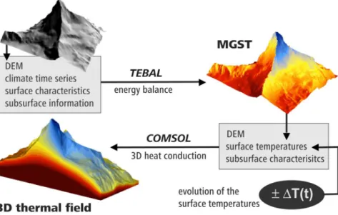
In this study, we used and further developed the approach described by Noetzli et al. (2007a; 2007b), which has been designed and tested for use in complex topography: A surface energy balance model and a heat-conduction model are coupled for forward simulation of a subsurface temperature field (Fig. 1). The TEBAL model (Gruber, 2005) calculates present mean ground surface temperatures (MGST). So calculated MGST

10

then serve as upper boundary condition in the heat conduction scheme, which we solve within the modeling package COMSOL. To account for the evolution of GST in the past, we compiled and simplified different GST histories, based on published changes in air temperatures and the assumption that GST follow these changes closely. Temporal variations of GST penetrate downward with amplitudes diminishing exponentially with

15

depth. In this study, we ignore seasonal temperature variations, which may penetrate down to about 12 m in bedrock (Gruber et al., 2004a), and only consider long-term variations of time scales of decades to millennia. Such long-term GST variations still occur on much shorter timescales than the geological processes that determine the geothermal heat flow. The past climatologic variations are therefore only treated as

20

transient effects of the upper boundaries in our model, and the lower basal heat flow boundary condition is kept constant (cf. Pollak and Huang, 2000). The lack of in-formation concerning the three-dimensional distribution of subsurface characteristics (thermo-physical properties, porosity, freezing characteristics, etc.) is approached by using model assumptions based on sensitivity studies.

25

We performed the basic simulations for a simplified ridge, the most common feature comprising alpine topography. A ridge of 1000 m height was set to an elevation of 3500 m a.s.l. and east-west orientation. Hence, it has a warm south-facing and a cold north-facing slope, which induces a subsurface temperature field with near vertical

(8)

TCD

2, 185–224, 2008

permafrost

Full Screen / Esc

isotherms in the uppermost part. The slope angle was set to 50◦_{, a typical value}

for rock slopes that do not accumulate a thick snow cover. To study the influence of terrain geometry, we varied the topographic factors (i.e., elevation and slope angle) of the two-dimensional ridge. Finally, we compared the results of the two-dimensional ridge topography to those for a flat and one-dimensional plain and a three-dimensional

5

pyramid geometry representing a simplified mountain peak.

3 Temperature modeling

3.1 Energy balance and rock surface temperature

The TEBAL model (Topography and Energy BALance, Gruber, 2005) simulates hourly time series of surface energy fluxes based on observed climate time series, topography,

10

and surface and subsurface information. The model is designed and validated for the calculation of near-surface temperatures in steep rock slopes in the Alps and was suc-cessfully applied in previous studies on bedrock permafrost (e.g., Gruber et al., 2004a; Noetzli et al., 2007b; Salzmann et al., 2007). MGSTs are computed with gridded digital elevation models (DEMs) of the topographies with a spatial resolution of 25 m

15

and with hourly climate time series from the high elevation meteo station Corvatsch (3315 m a.s.l.), Upper Engadine (Data source: MeteoSwiss) for the period 1990–1999 AD. We further reference this period as “today” or “present”. Surface and subsurface properties for bedrock were set according to Noetzli et al. (2007b). The simulation of the snow cover was neglected in this study, because we focus on steep rock slopes

20

that do not accumulate thick snow during winter (i.e., slopes angles of 50◦ _{and more).}

3.2 Heat conduction and subsurface temperature

In bedrock permafrost, heat transfer is mainly conductive and driven by the temper-ature variations at the surface and the heat flow from the interior of the Earth.

(9)

Fur-TCD

2, 185–224, 2008

permafrost

Full Screen / Esc

ther processes such as the effects of fluid flow can, as a first approximation, be ne-glected (Kukkonen and Safanda, 2001). Accordingly, we considered a conductive transient thermal field (Carslaw and Jaeger, 1959) in an isotropic and homogeneous medium under complex topography. The thermo-physical properties were set based on published values: thermal conductivity is 2.5 W K−1_m−1_{and volumetric heat}

capac-5

ity 2.0×106J m−3_K−1 _{(Cerm ´ak and Rybach, 1982; Wegmann et al., 1998; Safanda,}

1999).

Ice contained in the pore space and crevices delays the response to surface warm-ing by the consumption of latent heat, which may influence the time and depth scales of permafrost degradation by orders of magnitude even in low porosity rock (Wegmann

10

et al., 1998; Romanovsky and Osterkamp, 2000; Kukkonen and Safanda, 2001). This effect can be handled in heat transfer models by introducing an apparent heat capacity. We used the approach by Mottaghy and Rath (2006): The apparent heat capacity sub-stitutes the heat capacity in the heat transfer equation within the freezing interval w, where phase transition takes place, and which relates to the steepness of the unfrozen

15

water content curve. The parameter w makes it possible to account for a variety of ground conditions: Values typically range from 0.5 for material such as sand to 2 for material such as bentonite (Anderson and Tice, 1972; Williams and Smith, 1989), but information on bedrock material is sparse. Wegmann (1998) found that most of the interstitial ice in the rock of the Jungfrau East Ridge, Switzerland, freezes at −0.3◦_C,

20

which indicates a small freezing interval with a steep curve and a low value of w. A further controlling factor is the porosity of the material, for which we assumed 3% (vol-ume fraction, saturated conditions) to be a reasonable value to investigate the principal effects (Wegmann et al., 1998).

The finite-element (FE) modeling package COMSOL Multiphysics was used for

for-25

ward modeling of subsurface rock temperatures (Noetzli et al., 2007a). The FE mesh was created with increasing vertical refinement from 250 m at depth to 10 m for el-ements closest to the surface. In order to avoid effects from the model boundaries, a rectangle of 2000 m height and thermal insulation at its sides was added below.

(10)

TCD

2, 185–224, 2008

permafrost

Full Screen / Esc

The so created FE mesh consisted of about 1500 elements for a ridge, and of about 25 000 elements for a pyramid. The lower boundary condition was set to a uniform heat flux of 80 mW m2(Medici and Rybach, 1995), and for the upper boundary condi-tions the modeled MGSTs were given. The model was run with time-steps of 1 yr for simulations over a period of more than 1000 yr, and with time steps of 10 d for shorter

5

periods. Sensitivity runs with higher refinement of the FE mesh as well as changing to smaller time steps did not considerably change any of the results (the maximum absolute difference in modeled temperatures was below 0.1◦_C).

3.3 Evolution of surface temperature

A wealth of literature exists on temperature reconstructions from proxy data for global

10

(Pollak et al., 1998; Huang et al., 2000; Jones and Mann, 2004), hemispheric (Jones et al., 1998; Petit et al., 1999;), and regional scale (Patzelt, 1987; Isaksen et al., 2000; Casty et al., 2005) over the past centuries and millennia. For the European Alps, tem-perature variations are generally more pronounced with larger amplitudes compared to those averaged globally or for the Northern Hemisphere (Beniston et al., 1997;

Pfis-15

ter, 1999; Luterbacher et al., 2004). In the uppermost kilometers of the Earth’s crust, mainly the thermal effects of two events are prominent today (Haeberli et al., 1984): the temperature depression during the Pleistocene Ice Age and the sharp rise in temper-atures between the time of maximum glaciation (around 18 ky BP) and the beginning of the thermally more stable Holocene (around 10 ky BP). For the Holocene, the

Cli-20

matic Optimum (HCO, ca. 5–6 ky BP), the Medieval Warmth (MW, ca. 800–1300 AD), the Little Ice Age (LIA, ca. 1300–1850 AD), and the subsequent warming are typically resolved in temperature reconstructions (Dahl-Jensen et al., 1998). With increasing spatial and temporal refinement, climate variations become more complex and recon-structions more detailed, particularly towards the present time. This meets our needs

25

since a temperature signal entering into the subsurface is dampened with depth, that is, the temporal resolution of the surface temperature variations affecting subsurface temperatures decreases with depth.

(11)

TCD

2, 185–224, 2008

permafrost

Full Screen / Esc

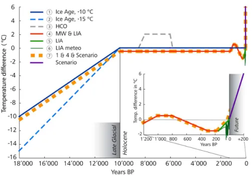
In this study, we analyze the influence of the above-mentioned periods (Fig. 2) on the present-day subsurface temperature field below steep mountains. The effects of temperature variations further back in time or of smaller amplitude are considered neg-ligible. For a detailed description of the most recent temperature fluctuations we used measured variations in mean annual air temperatures (MAAT) from a high alpine

sta-5

tion (Jungfraujoch, Switzerland, 3576 m a.s.l.), where air temperature data is available back to 1933 AD (Data Source: MeteoSchweiz). The difference in mean temperatures between the periods 1990–1999 AD and 1933–1950 AD amounts to +1◦_{C for this}

sta-tion. Additionally, we assumed a difference in air temperature of +0.5◦_{C between the}

end of the LIA and the start of the data recordings, resulting in a total increase of

10

+1.5◦_{C since 1850 AD (cf. Boehm et al., 2001).}

Based on these considerations, we analyzed the effect of the following temperature variations (Fig. 2):

– The Pleistocene Ice Age (1/2; numbers in brackets correspond to Fig. 2):

Temperature depressions are assumed −10◦_{C colder compared to present-day}

15

temperatures (Patzelt, 1987), followed by a linear increase from the time of maximum glaciation (18 ky BP) to the beginning of the Holocene (10 ky BP). For the Holocene no temperature variations were considered. To assess the effect of colder estimates, we additionally used a value of −15◦_{C (Haeberli et al., 1984).}

20

– HCO (3): During the Holocene Climate Optimum summer temperatures were

approx. 1.5–3◦_{C warmer than today (Burga, 1991). Mean annual temperatures}

probably were not as high, but to test the influence of this period we assumed +2◦_C.

25

– Past millennium (4): In contrast to e.g., von Rudloff (1980), newer studies

con-clude that air temperatures in Europe during the MW were probably not warmer than or comparable to today (Hughes and Diaz, 1994; Crowley and Lowery, 2000;

(12)

TCD

2, 185–224, 2008

permafrost

Full Screen / Esc

Goosse et al., 2006). Yet, to estimate its possible influence we used 0.5◦_{C higher}

surface temperatures than at present. For the LIA, we assumed temperatures 1.5◦_{C lower (Boehm et al., 2001).}

– Recent warming: We used a linear temperature increase following the LIA (5)

5

and, in addition, annual MAAT variations taken from meteodata (6).

In addition, we used a linear warming of the rock surface of +3◦_{C/100 yr for the next}

200 yr (Salzmann et al., 2007) to simulate a future subsurface temperature field.

4 Transient temperature fields below idealized topography

10

4.1 Effects of past climatic conditions

If not indicated otherwise, results are discussed and visualized for a ridge cross sec-tion of 1000 m height with a maximum elevasec-tion of 3500 m a.s.l., and a slope angle of 50◦_{. The subsurface material is assumed homogenous and isotropic, and no latent}

heat is considered. Variations from these basic settings are mentioned in the text and

15

indicated in the figures with checkboxes and corresponding abbreviations (i.e., “ini” for initialized, “lh” for latent heat considered, and “iso” for isotropic subsurface conditions). In general, the subsurface temperature pattern of a ridge does not vary greatly for dif-ferent GST histories and is characterized by the stationary temperature field. Initialized temperatures, however, are lower for the entire thermal field and all GST histories. In

20

Fig. 3, 0◦_{C and −3}◦_{C-isotherms of computed temperature fields initialized with different}

GST histories are compared to current GST stationary conditions. The 0◦_{C isotherm}

represents the permafrost boundary, whereas the −3◦_{C isotherm gives the temperature}

distribution inside the permafrost body. The temperature depression from the last Ice Age (1) is in the range of −0.5◦_{C for the upper half of the geometry, and in the range of}

(13)

TCD

2, 185–224, 2008

permafrost

Full Screen / Esc

−2.5◦C for the lower part. When assuming colder GST in the last Ice Age (2) these val-ues amount to −1◦

C and −4◦_{C, respectively. Simulating the GST variations during the}

Holocene (4) results in additionally lower temperatures: On the one hand, the LIA (5) is perceivable down to about 250 m depth. On the other hand, deeper parts are modeled colder because (1) and (2) do not consider that present-day GST are somewhat higher

5

than Holocene average. The effect of the HCO (3) on the temperatures is below 0.1◦_C

for the entire geometry, and results are therefore not displayed in Fig. 3. Results for GST history (6) do not notably differ from (5) and are not shown, either. Based on the results for (1) to (6), we compiled GST history (7), which takes into account the main GST variations that influence the subsurface thermal field in a high mountain ridge.

10

That is, the cold temperatures during the last Ice Age (1) and the major fluctuations in the past millennium (4). GST history (7) is used for all subsequent calculations and is referred to as “initialized” or “transient”.

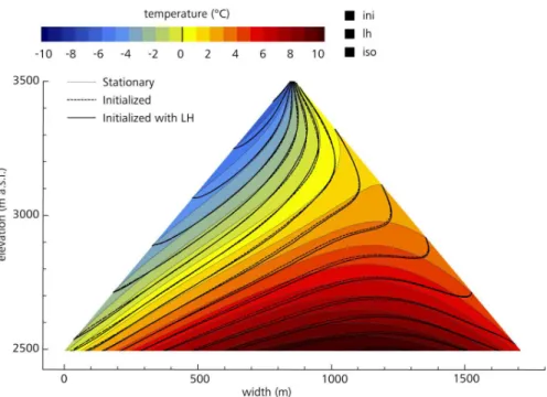
Figure 4 depicts the isotherms of the initialized temperature pattern together with the stationary field for current GST. The initialized temperature field is colder and in

15

the uppermost 100 m the recent warming since the LIA is clearly visible. In the middle part of the warmer side of the ridge, the inclination of the isotherms is reversed. In this part of the geometry, we identify the biggest differences compared to stationary condi-tions. The absolute temperature difference of a transient to a stationary thermal field for present-day GST is plotted in Fig. 5. Maximum calculated temperature depressions

20

in the innermost parts of the geometry are −3◦_{C, whereas the temperature depression}

does not exceed 1◦_{C in the upper half of the geometry. The MW and the fact that the}

LIA has not yet penetrated to great depth cause the warmer area visible in the top center of the ridge (Fig. 5).

4.1.1 Topography

25

For simulations based on conduction only, the elevation of the geometry changes the absolute temperature field but not its pattern. The temperature depressions given above are thus valid for ridge-topographies of any elevation, but the position of the

(14)

TCD

2, 185–224, 2008

permafrost

Full Screen / Esc

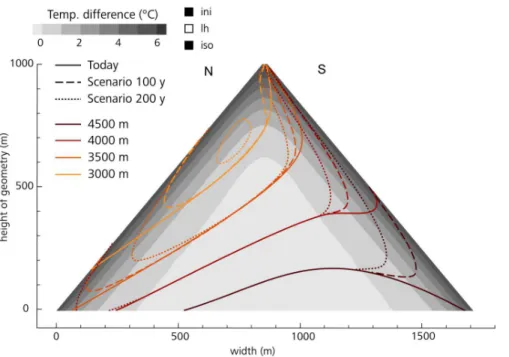
0◦_{C isotherm (or permafrost boundary) varies (Fig. 5). The difference in permafrost}

thickness (which we consider vertical to the surface) between stationary and transient results is bigger for higher mountains with deeper permafrost occurrence. For the high-est example shown in Fig. 5 (4500 m a.s.l.), the difference amounts to more than 100 m. For the lowest example (3000 m a.s.l.) it is still in the dimension of decameters.

5

Convex topography accelerates the reaction of the subsurface temperature to chang-ing surface conditions. Firstly and more obviously, the distance that a signal has to penetrate by conduction to reach the permafrost base in the interior of the mountain is shorter than in flat terrain. The steeper the topography, the shorter is this distance. In addition to this effect, the warming signal reaches the interior from more than one side,

10

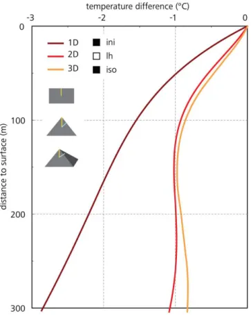
that is, from two sides in the case of a ridge, and from four sides in a pyramid-like situ-ation. To demonstrate this effect of multi-lateral warming, we compare the temperature depressions in T (z)-profiles in a flat one-dimensional plain, a two-dimensional ridge, and a three-dimensional pyramid (Fig. 6). For the two- and three-dimensional geom-etry, the profiles are extracted vertically from the top of the geometry. The resulting

15

temperature depression, however, was not plotted versus the length of the profile, but versus the shortest distance of the profile to the surface (cf. small schematic plots in Fig. 6). In this way, multi-lateral warming causes the effect shown, and not the fact that the distance to the surface is shorter than the depth of the profile. For the two mountain geometries the modeled temperature depression is roughly half of that for a flat plain

20

in the 200 m closest to the surface. For the deeper parts (i.e., 300 m and more), the difference increases and ca. −3◦

C for flat terrain contrast with ca. −1◦_{C for mountain}

topography. The effect of three-dimensional compared to two-dimensional geometry is small for the long time scale of the simulation and the depth range shown. This is due to the fact that the major part of the temperature signal has reached the depths shown

25

(15)

TCD

2, 185–224, 2008

permafrost

Full Screen / Esc

4.1.2 Subsurface properties

Information about subsurface properties (e.g., porosity, freezing characteristics) of bedrock is sparse for natural conditions in high mountains. In order to gain confidence in the modeling results, we tested their possible influence in sensitivity studies.

In low porosity material and for time scales of millennia, energy consumption due

5

to latent heat is of minor importance (Fig. 5): Subsurface temperatures are slightly colder, but differences to simulations without latent heat do not exceed 0.2◦_{C at depth.}

This is in accordance with calculations by Haeberli et al. (1984) or model experiments by Mottaghy and Rath (2006). The effect of latent heat only becomes important for transient simulations over shorter time periods (see below) or for considerably higher

10

porosities. In mountain permafrost areas, high ice contents may be present in the near surface layer, where porosity is often increased due to weathering and fracturing. For example, the ice content of the Schilthorn crest, Switzerland, is estimated to be 10– 20% in the upper meters and around 5% in the deeper parts (Hauck et al., 2008). We tested if this has an influence on the transient temperature field by adding a 15 m thick

15

layer with 20% porosity as a surface layer to the ridge geometry. Yet, no considerable difference to the simulations with homogenous porosity for the entire ridge resulted.

Thermal conductivities of bedrock often show large variations due to anisotropy (e.g., in gneiss). Values for the anisotropy factor of crystalline rocks are typically between 1.2 and 2 (Schoen, 1983; Kukkonen and Safanda, 2001). In order to investigate the

20

anisotropy effect on the initialized temperature field we performed model runs with thermal conductivity increased both horizontally and vertically (i.e., 3 W K−1_m−1 _and

2 W K−1_m−1 _{in the perpendicular direction). An increased horizontal thermal}

conduc-tivity supports lateral heat fluxes and the effect of steep topography, whereas an in-creased vertical component reduces it. The latter has a bigger effect on the modeled

25

temperatures at depth: Differences to isotropic conditions amount up to −2◦_{C for}

in-creased vertical thermal conductivity, and 0.5◦_{C for increased horizontal conductivity,}

(16)

TCD

2, 185–224, 2008

permafrost

Full Screen / Esc

The heat capacity of bedrock typically ranges from about 1.8 to 3×106J kg−1_K−1

(Cerm ´ak and Rybach, 1982). Test runs with these values result in a maximum differ-ence of less than 1◦_{C for the innermost part of the geometry.}

The geothermal heat flux has only little effect on the stationary subsurface temper-ature field inside steep mountain peaks (Noetzli et al., 2007b). This is also true for

5

transient calculations: Resulting temperature depressions from simulations with a zero heat flux lower boundary condition were assessed to differ less than 0.2◦_{C. Moreover,}

we tested the influence of radiogenetic heat production. Values for rock are given be-tween 0.5 and 6 µW m−3 _{(Kohl, 1999). We used a medium value of 3 µW m}−3 _{for a}

test run. Maximum differences to results without heat production were assessed to be

10

below 0.5◦_{C for the entire ridge, and below 0.1}◦_{C for the upper half.}

4.2 Effects of future warming

The effect of an assumed linear temperature rise of +3◦_{C/100 yr during 200 yr has been}

shown by Noetzli et al. (2007b). The warming has penetrated to a depth of approxi-mately 250 m, but only about 50% of the temperature change has reached a depth of

15

more than 100 m. Temperatures at greater depth still remain unchanged. Further, a re-tarding influence of latent heat was demonstrated. In this study, we analyzed the effect of elevation, geometry, and subsurface conditions on future transient thermal fields in high-mountains.

4.2.1 Topography

20

The state of the permafrost body inside ridges of different elevations in 200 yr is dis-played schematically in Fig. 8. The position of the 0◦_{C isotherm 250 m or less below}

the surface changes drastically and is bent towards the top. On the warmer side of the ridge, the isotherms first change to lie more or less parallel to the surface and then move rather uniformly towards the colder side. For all elevations modeled, no

25

(17)

TCD

2, 185–224, 2008

permafrost

Full Screen / Esc

permafrost occurrence remains below the surface for a long time, especially for higher elevations. For lower topographies relict permafrost remains on the colder side.

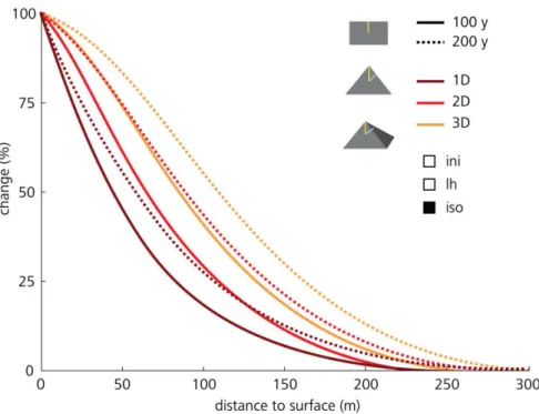
The above-described effect of multi-lateral warming is also significant for shorter time periods. Figure 9 displays the percentage of a surface temperature signal that has reached a certain depth after 100 and 200 yr, respectively. For example, 50% of the

5

temperature signal has reached a depth of about 60 m after 200 yr in a one-dimensional vertical simulation. In the two-dimensional situation, it has already penetrated to about 90 m, and in the three-dimensional situation to ca. 115 m. In the same way as in Fig. 6, values for the two- and three-dimensional geometries are plotted versus the shortest distance to the surface, rather than versus the length of the extracted profile.

10

4.2.2 Subsurface conditions

The effect of latent heat on future temperature fields is illustrated in Fig. 10. With varying freezing range (parameter w) the size of the modeled permafrost body does not change much, but the temperature distribution inside changes. A smaller value of w (i.e., a smaller freezing range and a steeper unfrozen water content curve) keeps

15

the thermal field in the temperature range little below the melting point for a longer time period. This leads to more homogeneous temperature fields in warming permafrost than when modeled with a larger value of w. In terms of T (z)-profiles from boreholes this results in steeper profiles and smaller temperature gradients with depth (Fig. 11). For example, this effect can be observed in the temperature profiles of the two 100 m

20

deep boreholes on the Schilthorn crest (Switzerland), which are entirely in the range of −2 to 0◦_{C. This points to a small freezing interval and a low value of w (Noetzli et}

al., 2008). The observed high ice-content in the near-surface layer (cf. Sect. 4.1.2) can act as a buffer to temperature changes at the surface and further delay the short-term reaction of the subsurface temperature field (Fig. 11).

(18)

TCD

2, 185–224, 2008

permafrost

Full Screen / Esc

5 Permafrost distribution and evolution in the Matterhorn

The Matterhorn (4478 m a.s.l.) in Switzerland is probably the most prominent mountain peak in the European Alps. Its distinctive topography resembles a pyramid of about 1500 m height and faces exposed to all four main orientations. Slope angles are >45◦_C

for the most parts and only isolated and small patches of snow persist on the rock. With

5

this extreme three-dimensional geometry, the Matterhorn constitutes a prime example for an application of the presented modeling approach to real topography.

A north-south cross section through the modeled subsurface temperature field of the Matterhorn for today and in 200 yr is given in Fig. 12. Surface temperatures were mod-eled using climate time series from the Corvatsch (data source: MeteoSwiss), which

10

is located in a central Alpine climate similar to the Matterhorn area (cf. Gruber et al., 2004b). Surface properties were used according to the previous simulations and Noet-zli et al. (2007b). The topography was taken from the 25 m DEM Level 2 by Swisstopo and the FE mesh contained nearly 55 000 elements. The lithology of the Matterhorn mainly consists of gneiss and granite of the east Alpine Dent-Blanche nappe. We set a

15

thermal conductivity of 2.5 W m−1_K−1_{, a volumetric heat capacity of 2.2×106 J m}−3_K−1_,

a porosity of 3%, and w=2. Boundary conditions and time steps were the same as in the simulations presented above, and anisotropy was not considered.

The extreme geometry of the Matterhorn leads to a strongly three-dimensional sub-surface temperature field, which is characterized by steeply inclined isotherms, a strong

20

heat flux from the south to the north face, and a smaller heat flux from the east to the west face. For current conditions, the entire mountain is within permafrost, except for the lowest parts of the southern side. For the calculated scenario, in contrast, no per-mafrost remains at the surface on the southern side after 200 yr. On the northern side, the permafrost boundary at the surface has risen to an elevation of about 3500 m a.s.l.

25

However, both on the south and the north side, substantial permafrost remains a few decameters below the surface. Temperatures of the remaining permafrost body are warming and the extent of so-called warm permafrost (i.e., about −2 to 0◦_{C) is}

(19)

signifi-TCD

2, 185–224, 2008

permafrost

Full Screen / Esc

cantly increasing in volume as well as in vertical extent (Fig. 13).

6 Discussion

With the experiments conducted in this study we analyzed the influence of combined transient and three-dimensional topography effects on the subsurface temperature field in mountain permafrost. For the correct interpretation of the results, a number of

uncer-5

tainties and limitations of the modeling approach are important, which are discussed in the following.

Instrumental records of climate parameters are typically available for the past ca. 100 yr. Reconstructions of pre-industrial climate rely on proxy data and are sub-ject to a great number of uncertainties, which may be even larger than the influence a

10

certain time period has on the subsurface temperatures. In general, climate reconstruc-tion studies agree well on the shape of the climate fluctuareconstruc-tions, whereas the absolute amplitude of the temperature variations ranges significantly (Esper et al., 2005). Fur-ther, we assumed that changes in GST closely follow air temperatures. Salzmann et al. (2007) demonstrated a considerable influence of topography on the reaction of

sur-15

face temperatures in steep rock to changing atmospheric conditions. The dimensions of the GST changes, however, are not influenced, and in view of the above-mentioned uncertainties of the reconstructed amplitudes of temperature variations, we consider this effect to be less important for this study.

For the scenario calculations we assumed a linear temperature rise of +3◦_{C in 100 yr.}

20

An exponential temperature rise as generally proposed for climate change scenarios may slow down the temperature changes calculated. Contrastingly, the temperature increase assumed represents a mean change in GST of bedrock in Alpine terrain for different climate scenarios (Salzmann et al., 2007) and is at the lower range of the scenarios presented for air temperature change by IPCC (2007), where a double

tem-25

perature rise is not considered unrealistic or extreme for the Alps.

(20)

TCD

2, 185–224, 2008

permafrost

Full Screen / Esc

study. Haeberli (1983) points to higher temperatures at a glacier base than for rock exposed directly to the atmosphere during the past cold periods and, hence, paleocli-matic effects below previously glacier-covered areas are smaller. This may be impor-tant, for example, for the lower parts of the Matterhorn. Further, snow that may remain in steep bedrock can have a cooling effect on steep slopes even in summer (Gruber

5

and Haeberli, 2007). This cooling effect, however, has not yet been quantified.

In terms of subsurface characteristics, errors induced by uncertain assumptions of thermal conductivity, heat capacity, and heat production increase with depth and length of the simulation, whereas errors caused by uncertainties in subsurface ice decrease. Information on the amount and freezing characteristics of subsurface ice in bedrock is

10

required to improve realistic modeling, but is still scarce. The joint interpretation of nu-merical model results with data from geophysical monitoring (e.g., electrical resistivity tomography, ERT) has been successfully realized for a first case study of the Schilthorn crest in the Swiss Alps (Noetzli et al., 2008), and information gained in this way can improve the representation of the subsurface in the model.

15

Neglecting water circulation along the joint systems of bedrock is an important lim-itation of the approach used. For example, advective heat transfer along clefts can contribute to subsurface heat transfer and lead to thaw corridors in permafrost, which substantially modify a purely conductive system (Gruber et al., 2004a; Gruber and Haeberli, 2007). First applications of geophysical monitoring in solid rock walls

re-20

cently identified thawed cleft systems influenced by moving water (Krautblatter and Hauck, 2007). Process understanding of advective heat transfer processes in steep bedrock permafrost, however, is limited.

Because of its temperature range, the acceleration of subsurface temperature changes through multi-lateral warming, and the virtual decoupling of the mountain

25

from the geothermal heat flux, bedrock permafrost in high mountains is particularly sensitive to climate change. Simulations of possible future subsurface temperatures il-lustrate the long lasting and deep-reaching changes in the subsurface thermal field and point to hardly any remaining permafrost at the surface on south-facing Alpine slopes

(21)

TCD

2, 185–224, 2008

permafrost

Full Screen / Esc

in 200 yr. Permafrost boundaries are about to lie surface-parallel in the top parts of the mountains and then move rather uniformly towards the colder side. In terms of temperature-related instabilities such a thawing and horizontally migrating permafrost table may be delicate: rock volumes with temperatures close to the melting point, pos-sibly containing critical ice-water-rock mixtures, increase and may extend over large

5

vertical distances up to entire mountain flanks. For the Matterhorn, for example, warm permafrost exists today in the middle of the southern side, where rock fall events actu-ally have been observed in recent years (2003 and 2006). In the calculated scenario, the warm permafrost zone extends over the entire south face and, in addition, over large parts of the north face.

10

7 Conclusions and perspectives

The results of the simulations performed in this study lead to the following conclusions:

– The main variations in surface temperatures that influence present-day

subsur-face temperatures in Alpine permafrost are the last glacial period and the major temperature variations in the past millennium.

15

– Transient paleothermal effects caused by past climate variations exist in the

inte-rior of high-mountain peaks. Modeled temperature depressions at a distance of 500 m from the surface are in the range of −3◦_{C compared stationary conditions}

from present-day GST.

20

– For temperature fields influenced by future warming, transient effects are more

important. Scenarios point to temperature fields that are characterized by long-term and deep reaching perturbations and by temperature patterns that strongly deviate from stationary conditions.

(22)

TCD

2, 185–224, 2008

permafrost

Full Screen / Esc

– Two- and three-dimensional topography significantly accelerates the pace of a

surface temperature signal entering into the subsurface. Together with the fast and unfiltered reaction of its surface to changes in atmospheric conditions and the low ice content, this makes bedrock permafrost in high mountains particularly sensitive to degradation.

5

– In low porosity rock, the influence of latent heat on the temperature depressions

caused by past GST variations is too small to be important and can be neglected. In connection with probable future warming, however, latent heat effects modify the pace of permafrost degradation considerably.

10

– Temperatures of the permafrost body are warming in the calculated scenario,

and the extent of warm permafrost is significantly increasing in volume as well as in vertical extent.

15

– The distribution and extent of temperatures little below the melting point in

warm-ing permafrost is determined by the freezwarm-ing characteristics of the subsurface material. A small freezing range leads to more homogenous temperature fields and T (z)-profiles with small temperature gradients.

20

The investigation of mountain permafrost by transient three-dimensional modeling has only been used for a few case studies of real mountain topography so far. It bears potential for various applications that require knowledge of current and future thermal conditions of mountain permafrost, for instance, the reanalysis of the thermal condi-tions in rock fall starting zones located in permafrost areas, the improved interpretation

25

of T (z)-profiles measured in boreholes, and the assessment of thermal conditions and their evolution in rock below infrastructure. The limitations and uncertainties discussed

(23)

TCD

2, 185–224, 2008

permafrost

Full Screen / Esc

above call for improved knowledge of subsurface properties in bedrock permafrost, as well as for enhanced validation and modeling practices. A promising approach may be the combination of numerical modeling together with measurements and interpretation of field data. For example, the representation of the subsurface physical properties in the model can be improved by incorporating subsurface information (e.g., geological

5

structures, water/ice content) detected by geophysical surveys. Further, process un-derstanding and incorporation of advective heat transfer and snow remaining in steep rock will be important for realistic modeling of subsurface temperature field.

Acknowledgements. This study was supported by the Swiss National Science Foundation,

as part of the NF 20-10796./1 project “Frozen rock walls and climate change: transient

3-10

dimensional investigation of permafrost degradation”. Special thanks go to S. Friedel for sup-port with the COMSOL software and for providing an imsup-port routine for DEMs. Fruitful discus-sions with W. Haeberli and M. Hoelzle contributed to the development of this study.

References

Anderson, D. M. and Tice, A. R.: Predicting unfrozen water contents in frozen soils from surface

15

area measurements, Highway Research Record, 393, 12–18, 1972.

Beltrami, H.: On the relationship between ground temperature histories and meteorological records: A report on the Pomquet Station, Global Planet. Change, 29, 327–348, 2001. Beltrami, H., Ferguson, G., and Harris, R. N.: Long-term tracking of climate change by

under-ground temperatures, Geophys. Res. Lett., 32, doi:10.1029/2005GL023714, 2005.

20

Beniston, M., Diaz, H. F., and Bradley, R. S.: Climatic change at high elevation sites: An overview, Climatic Change, 36, 233–251, 1997.

Beniston, M.: Mountain climates and climate change: An overview of processes focusing on the European Alps, Pure Appl. Geophys., 162, 1587–1606, 2005.

Birch, F.: The effects of Pleistocene climatic variations upon geothermal gradients, Am. J. Sci.,

25

246, 729–760, 1948.

Boehm, R., Auer, I., Brunetti, M., Maugeri, M., Nanni, T., and Schoener, W.: Regional tem-perature variability in the European Alps: 1760–1998 from homogenized instrumental time series, Int. J. Climatol., 21, 1779–1801, 2001.

(24)

TCD

2, 185–224, 2008

permafrost

Full Screen / Esc

Burga, C.: Vegetation history and paleoclimatology of the middle Holocene: Pollen analysis of Alpine peat bog sediments, covered formerly by the Rutor Glacier, 2510 m (Aosta Valley, Italy), Global Ecol. Biogeogr., 1, 143–150, 1991.

Carslaw, H. S. and Jaeger, J. C.: Conduction of heat in solids, Oxford science publications, Clarendon Press, Oxford, 510 pp., 1959.

5

Casty, C., Wanner, H., Luterbacher, L., Esper, J., and Boehm, R.: Temperature and precipitation variability in the European Alps since 1500, Int. J. Climatol., 25, 1855–1880, 2005.

Cerm ´ak, V. and Rybach, L.: Thermal conductivity and specific heat of minerals and rocks, in: Landolt-b ¨ornstein Zahlenwerte und Funktionen aus Naturwissenschaften und Technik, neue Serie, physikalische Eigenschaften der Gesteine (v/1a), edited by: Angeneister, G., Springer,

10

Berlin, 305–343, 1982.

Crowley, T. J. and Lowery, T. S.: How warm was the Medieval Warm Period? Ambio, 29, 51–54, 2000.

Dahl-Jensen, D., Modegaard, K., Gundestrup, N., Clow, G. D., Johnsen, S. J., Hansen, A. W., and Balling, N.: Past temperatures directly from the Greenland Ice Sheet, Science, 282,

15

268–271, 1998.

Davies, M. C. R., Hamza, O., and Harris, C.: The effect of rise in mean annual temperature on the stability of rock slopes containing ice-filled discontinuities, Permafrost Periglac., 12, 137–144, 2001.

Esper, J., Wilson, R. J. S., Frank, D. C., Moberg, A., Wanner, H., and Luterbacher, J.: Climate:

20

Past ranges and future changes, Quarternary Sci. Rev., 24, 2164–2166, 2005.

Goosse, H., Arzel, O., Luterbacher, J., Mann, M. E., Renssen, H., Riedwyl, N., Timmermann, A., Xoplaxi, E., and Wanner, H.: The origin of the European “Medieval Warm Period”, Clim. Past, 2, 99–113, 2006,

http://www.clim-past.net/2/99/2006/.

25

Gruber, S., Hoelzle, M., and Haeberli, W.: Permafrost thaw and destabilization of Alpine rock walls in the hot summer of 2003, Geophys. Res. Lett., 31, doi:10.1029/2004GL0250051, 2004a.

Gruber, S., Hoelzle, M., and Haeberli, W.: Rock wall temperatures in the Alps: Modeling their topographic distribution and regional differences, Permafrost Periglac., 15, 299–307, 2004b.

30

Gruber, S., King, L., Kohl, T., Herz, T., Haeberli, W., and Hoelzle, M.: Interpretation of geothermal profiles perturbed by topography: The Alpine permafrost boreholes at Stockhorn Plateau, Switzerland, Permafrost Periglac., 15, 349–357, 2004c.

(25)

TCD

2, 185–224, 2008

permafrost

Full Screen / Esc

Gruber, S.: Mountain permafrost: Transient spatial modelling, model verification and the use of remote sensing, Department of Geography, University of Zurich, Zurich, 2005.

Gruber, S. and Haeberli, W.: Permafrost in steep bedrock slopes and its temperature-related destabilization following climate change, J. Geophys. Res., 112, doi:10.1029/2006JF000547, 2007.

5

Haeberli, W.: Permafrost-glacier relationships in the Swiss Alps – today and in the past, 4th International Conference on Permafrost, Proceedings, Fairbanks, Alaska, 415–420, 1983. Haeberli, W., Rellstab, W., and Harrison, W. D.: Geothermal effects of 18 ka BP ice conditions

in the Swiss Plateau, Ann. Glaciol., 5, 56–60, 1984.

Haeberli, W.: Construction, environmental problems and natural hazards in periglacial

moun-10

tain belts, Permafrost Periglac., 3, 111–124, 1992.

Haeberli, W., Wegmann, M., and Vonder M ¨uhll, D.: Slope stability problems related to glacier shrinkage and permafrost degradation in the Alps, Eclogae Geol. Helv., 90, 407–414, 1997. Haeberli, W. and Beniston, M.: Climate change and its impacts on glaciers and permafrost in

the Alps, in: Ambio – a journal of the human environment, edited by: Rapp, A., and Kessler,

15

E., 4, The Royal Swedish Academy of Sciences, 258–265, 1998.

Harris, C., Davies, M. C. R., and Etzelm ¨uller, B.: The assessment of potential geotechnical haz-ards associated with mountain permafrost in a warming global climate, Permafrost Periglac., 12, 145–156, 2001.

Hauck, C., Bach, M., and Hilbich, C.: A 4-phase model to quantify subsurface ice and water

20

content in permafrost regions based on geophyiscal datasets, 9th International Conference on Permafrost, Fairbanks, US, in press, 2008.

Huang, S., Pollak, H. N., and Shen, P. Y.: Temperature trends over the last five centuries reconstructed from borehole temperatures, Nature, 403, 756–758, 2000.

Hughes, M. K. and Diaz, H. F.: Was there a “Medieval Warm Period”, and if so, where and

25

when?, Climatic Change, 26, 109–142, 1994.

IPCC: Climate change 2007: The physical science basis. Contribution of working group I to the fourth assessment report of the Intergovernmental Panel on Climate Change, edited by: Solomon, S., Qin, D., Manning, M., Chen, Z., Marquis, M., Averyt, K. B., Tignor, M., and Miller, H. L., Cambridge University Press, Cambridge, United Kingdom and New York, 996

30

pp., 2007.

Isaksen, K., Vonder M ¨uhll, D., Gubler, H., Kohl, T., and Sollid, J. L.: Ground surface temper-ature reconstruction based on data from a deep borehole in permafrost at Janssonhaugen,

(26)

TCD

2, 185–224, 2008

permafrost

Full Screen / Esc

Svalbard, Ann. Glaciol., 31, 287–294, 2000.

Isaksen, K., Sollid, J. L., Holmlund, P., and Harris, C.: Recent warming of mountain permafrost in Svalbard and Scandinavia, J. Geophys. Res., F02S04, doi:10.1029/2006JF000522, 2007. Jones, P. D., Briffa, K. R., Barnett, T. P., and Tett, S. F. B.: High-resolution paleoclimatic records

for the last millennium: Interpretation, integration, and comparison with general circulation

5

model control-run temperatures, Holocene, 8, 455–471, 1998.

Jones, P. D. and Mann, M. E.: Climate over past millennia, Rev. Geophys., 42, RG2002, doi:2010.1025/2003RG000143, 2004.

Kohl, T.: Transient thermal effects at complex topographies, Tectonophysics, 306, 311–324, 1999.

10

Kohl, T., Signorelli, S., and Rybach, L.: Three-dimensional (3-D) thermal investigation below high Alpine topography, Phys. Earth Planet. In., 126, 195–210, 2001.

Kohl, T. and Gruber, S.: Evidence of paleaotemperature signals in mountain permafrost areas, 8th International Conference on Permafrost, Extended Abstracts, Z ¨urich, 83–84, 2003. Krautblatter, M. and Hauck, C.: Electrical resistivity tomography monitoring of permafrost in

15

solid rock walls, J. Geophys. Res., 112, doi:10.1029/2006JF000546, 2007.

Kukkonen, I. T. and Safanda, J.: Numerical modelling of permafrost in bedrock in northern Fennoscandia during the Holocene, Global Planet. Change, 29, 259–273, 2001.

Lachenbruch, A. H. and Marshall, B. V.: Changing climate: Geothermal evidence from per-mafrost in the alaskan arctic, Science, 234, 689–696, 1986.

20

Luethi, M. and Funk., M.: Modelling heat flow in a cold, high-altitude glacier: Interpretation of measurements from Colle Gnifetti, Swiss Alps, J. Glaciol., 47, 314–324, 2001.

Lunardini, V. J.: Climatic warming and the degradation of warm permafrost, Permafrost Periglac., 7, 311–320, 1996.

Luterbacher, J., Dietrich, D., Xoplaxi, E., Grosjean, M., and Wanner, H.: European seasonal

25

and annual temperature variability, trends and extremes since 1500, Science, 303, 1499– 1503, 2004.

Medici, F. and Rybach, L.: Geothermal map of Switzerland 1995 (heat flow density), G ´eophysique 30, Schweizerische Geophysikalische Kommission, 1995.

Mottaghy, D. and Rath, V.: Latent heat effects in subsurface heat transport modeling and their

30

impact on paleotemperature reconstructions, Geophys. J. Int., 164, 236–245, 2006.

Noetzli, J., Hoelzle, M., and Haeberli, W.: Mountain permafrost and recent Alpine rock-fall events: A GIS-based approach to determine critical factors, 8th International Conference on

(27)

TCD

2, 185–224, 2008

permafrost

Full Screen / Esc

Permafrost, Proceedings, Z ¨urich, 827–832, 2003.

Noetzli, J., Gruber, S., and Friedel, S.: Modeling transient permafrost temperatures below steep alpine topography, COMSOL User Conference, Grenoble, 139–143, 2007a.

Noetzli, J., Gruber, S., Kohl, T., Salzmann, N., and Haeberli, W.: Three-dimensional distribution and evolution of permafrost temperatures in idealized high-mountain topography, J. Geophys.

5

Res., 112, doi:10.1029/2006JF000545, 2007b.

Noetzli, J., Hilbich, C., Hauck, C., Hoelzle, M., and Gruber, S.: Comparison of simulated 2D temperature profiles with time-lapse electrical resistivity data at the Schilthorn crest, Switzer-land., 9th International Conference on Permafrost, Fairbanks, US, in press, 2008.

Patzelt, G.: Neue Ergebnisse der Sp ¨at- und Postglazialforschuung in Tirol, in: Jahresbericht,

10

¨

Osterreichische Geographische Gesellschaft, Zweigverein Innsbruck, 11–18, 1987.

PERMOS: Permafrost in Switzerland 2002/2003 and 2003/2004, Glaciological report (Per-mafrost) no. 4/5 of the Cryospheric Commission of the Swiss Academy of Sciences (SCNAT) and Department of Geography, University of Zurich, edited by: Vonder Muehll, D., Noetzli, J., Roer, I., Makowski, K., and Delaloye, R., 104 pp., 2007.

15

Petit, J. R., Jouzel, J., Raynnaud, D., Barkov, N. I., Barnola, J.-M., Basile, I., Bender, M., Chap-pellaz, J., Davis, M., Delaygue, G., Delmotte, M., Kotlyakov, V. M., Legrand, M., Lipenkov, V. Y., Lorius, C., P ´epin, L., Ritz, C., Saltzman, E., and Stievenard, M.: Climate and atmospheric history of the past 420 000 years from the Vostok ice core, Antarctica, Nature, 399, 429–436, 1999.

20

Pfister, C.: Wetternachhersage, Haupt, Bern, 304 pp., 1999.

Pollak, H. N., Huang, S., and Shen, P. Y.: Climate change record in subsurface temperatures: A global perspective, Science, 282, 279–281, 1998.

Pollak, H. N. and Huang, J.: Climate reconstruction from subsurface temperatures, Ann. Rev. Earth Planet. Sci., 28, 339–365, 2000.

25

Romanovsky, V. E. and Osterkamp, T. E.: Effects of unfrozen water on heat and mass transport processes in the active layer and permafrost, Permafrost Periglac., 11, 219–239, 2000. Romanovsky, V. E., Gruber, S., Instanes, A., Jin, H., Marchenko, S. S., Smith, S. L., Trombotto,

D., and Walter, K. M.: Frozen ground, in: Global outlook for ice and snow, edited by: UNEP, UNEP/GRID-Arendal, Norway, 182–200, 2007.

30

Safanda, J.: Ground surface temperature as a function of slope angle and slope orientation and its effect on the subsurface temperature field, Tectonophysics, 306, 367–375, 1999. Safanda, J. and Rajver, D.: Signature of the last ice age in the present subsurface temperatures

(28)

TCD

2, 185–224, 2008

permafrost

Full Screen / Esc

in the Czech Republic and Slovenia, Global Planet. Change, 29, 241–257, 2001.

Salzmann, N., Noetzli, J., Gruber, S., Hauck, C., and Haeberli, W.: RCM-based ground tem-perature scenarios in high-mountain topography and their uncertainty ranges, J. Geophys. Res., 112, doi:10.1029/2006JF000527, 2007.

Schoen, J.: Petrophysik, Ferdinand Enke, Stuttgart, 405 pp., 1983.

5

Von Rudloff, H.: Das Klima – Entwicklung in den letzten Jahrhunderten im mitteleurop ¨aischen Raume (mit einem R ¨uckblick auf die postglaziale Periode), in: Das Klima – Analysen und Modelle, Geschichte und Zukunft, edited by: Oeschger, H., Messerli, B., and Silvar, M., Springer, Berlin, 125–148, 1980.

Wegmann, M.: Frostdynamik in hochalpinen Felsw ¨anden am Beispiel der Region

Jungfraujoch-10

Aletsch, 161, Versuchsanstalt f ür Wasserbau, Hydrologie und Glaziologie der ETH Z ürich, ETH Z ürich, Z ürich, 143 pp., 1998.

Wegmann, M., Gudmundsson, G. H., and Haeberli, W.: Permafrost changes in rock walls and the retreat of alpine glaciers: A thermal modelling approach, Permafrost Periglac., 9, 23–33, 1998.

15

Williams, P. J. and Smith, M. W.: The frozen earth, 1 ed., Studies in polar research, Cambridge University Press, Cambridge, 306 pp., 1989.

(29)

TCD

2, 185–224, 2008

permafrost

Full Screen / Esc

Fig. 1. Mean ground surface temperatures (MGST) are modeled based on a surface energy balance model (TEBAL). They are used as upper boundary condition in a three-dimensional finite element heat conduction scheme (within COMSOL) to compute the subsurface tempera-ture field. For transient simulations the evolution of the surface temperatempera-tures is prescribed.

(30)

TCD

2, 185–224, 2008

permafrost

Full Screen / Esc

Fig. 2. For the initialization runs, surface temperature histories of diverse lengths and temporal resolutions were used. Based on the results obtained, an initialization curve for further simula-tions was compiled (thick dashed orange line). Scenarios were calculated assuming a uniform linear warming of +3◦_{C/100 yr. MW=Medieval Warmth, HCO=Holocene Climate Optimum,}

(31)

TCD

2, 185–224, 2008

permafrost

Full Screen / Esc

Fig. 3. Difference in the subsurface temperature field for a stationary simulation compared to model runs using different surface temperature histories: The 0◦_{C and −3}◦_{C isotherms for the}

(32)

TCD

2, 185–224, 2008

permafrost

Full Screen / Esc

Fig. 4. The isotherms of a stationary temperature field (thin grey lines and background colors) compared to an initialized one (temperature history (7) from Fig. 2). The transient temperature field is shown for simulations both with (solid line) and without (dotted line) considering the effects of latent heat. The porosity was set to 3%.

(33)

TCD

2, 185–224, 2008

permafrost

Full Screen / Esc

Fig. 5. The difference of the stationary solution to an initialized one (temperature history 7 from Fig. 2) is shown in gray colors. The lines indicate the permafrost boundary for the stationary (dotted line) and the transient (solid line) simulation, respectively, for four different maximum elevations of a ridge ranging from 3000 to 4500 m a.s.l. Colors indicate different elevations.

(34)

TCD

2, 185–224, 2008

permafrost

Full Screen / Esc

Fig. 6. Temperature depression in the subsurface thermal field of today caused by colder past surface temperatures for one- (flat terrain), two- (ridge), and three-dimensional (pyramid) situations. In the two- and three-dimensional situations, profiles are extracted vertically from the top of the geometry. Temperature differences are plotted versus the shortest distance to the surface, i.e., the distance the temperature signal penetrated.