Water isotope module of the ECHAM atmospheric general circulation model: A study on timescales from days to several years

HAL Id: hal-03119631

https://hal.archives-ouvertes.fr/hal-03119631

Submitted on 25 Jan 2021

HAL is a multi-disciplinary open access

archive for the deposit and dissemination of

sci-entific research documents, whether they are

pub-lished or not. The documents may come from

teaching and research institutions in France or

abroad, or from public or private research centers.

L’archive ouverte pluridisciplinaire HAL, est

destinée au dépôt et à la diffusion de documents

scientifiques de niveau recherche, publiés ou non,

émanant des établissements d’enseignement et de

recherche français ou étrangers, des laboratoires

publics ou privés.

Water isotope module of the ECHAM atmospheric

general circulation model: A study on timescales from

days to several years

G. Hoffmann, M. Werner, M. Heimann

To cite this version:

G. Hoffmann, M. Werner, M. Heimann. Water isotope module of the ECHAM atmospheric general

circulation model: A study on timescales from days to several years. Journal of Geophysical Research:

Atmospheres, American Geophysical Union, 1998, 103 (D14), pp.16871-16896. �10.1029/98JD00423�.

�hal-03119631�

JOURNAL OF GEOPHYSICAL RESEARCH, VOL. 103, NO. D14, PAGES 16,871-16,896, JULY 27, 1998

Water isotope module of the ECHAM

atmospheric

general circulation model:

A study on timescales from days to several years

G. Hoffmann

Laboratoire des Sciences du Climat et de l'Environnement, CEA/CNRS, Centre d'Etudes de Saclay, Gif sur Yvette, France

M. Werner and M. Heimann

Max Planck Institut fiir Meteorologie, Hamburg, Germany

Abstract. Results are presented of a global simulation of the stable water isotopes

H•80 and HD160 as implemented

in the hydrological

cycle

of the ECHAM atmo-

spheric general circulation model. The ECHAM model was run under present-day

climate conditions

at two spatial resolutions

(T42,T21), and the simulation

results

are compared

with observations.

The high-resolution

model (T42) more realistically

reproduced the observations, thus demonstrating that an improved representation

of advection and orography is critical when modeling the global isotopic water cycle.

The deuterium

excess

(d=SD-8*5180)

in precipitation

offers

additional

information

on climate conditions

(e.g., relative humidity and temperature) which prevailed at

evaporative sites. Globally, the simulated deuterium excess agrees fairly well with observations showing maxima in the interior of Asia and minima in cold marine regions. However, over Greenland the model failed to show the observed seasonality of the excess and its phase relation to 5D reflecting either unrealistic source areas modeled for Greenland precipitation or inadequate description of kinetics in the

isotope module. When the coarse

resolution

model (T21) is forced with observed

sea surface temperatures from the period 1979 to 1988, it reproduced the observed weak positive correlation between the isotopic signal and the temperature as well as the weak negative anticorrelation between the isotopic signal and the precipita- tion. This model simulation further demonstrates that the strongest interannual climate anomaly, the E1 Nifio Southern Oscillation, imprints a strong signal on the water isotopes. In the central Pacific the anticorrelation between the anomalous precipitation and the isotope signal reaches a maximum value of-0.8.

1. Introduction

Since more than a decade, a useful modeling tool in isotope geochemistry has been available: water iso- tope modules built into atmospheric general circula-

tion models (AGCMs). The pioneering work was pub-

lished by Youssaume e! al. [1984]. For the first time,

it presented the isotopic composition of precipitation under present-day climate conditions as modeled glob- ally by an AGCM, the model of the Laboratoire de

M4t4orologie Dynamique (LMD). Such isotope mod-

ules incorporate the well-known physics of fractiona- tion of water isotopes into the hydrological cycle of AGCMs. The principal isotopic components of water

are H•O, HDI•O (deuterium,

approximately

0.5ø•o

Copyright 1998 by the American Geophysical Union. Paper number 98JD00423.

0148-0227 / 98 / 98 J D-00423 $ 09.00

of the water on the Earth), H}80 (m 2ø•o of all wa-

ter) and the radioactive

tritium HT160(usually

the

isotopic composition of water is expressed as devia- tion from a standard, V-SMOW, the Vienna standard

mean ocean water. For example,

for H}80, 5180=

[

(180/160)Sample/(

18 I O)V_SMOW_

O/ 6

1.]

and,

cor-

respondingly,

6D for HDlSO.). The isotopic

composi-

tion of atmospheric water is a passive tracer and is influ- enced by a variety of climate parameters such as tem- perature, humidity and precipitation. Both the equi-

librium fractionation of water isotopes during evapora-

tion and the condensation [Majoube, 1971a, b] and ki-

netic, "nonequilibrium" effects [Stewart, 1975;Jouzel

and Merlivat, 1984] are sufficiently known from labora-

tory experiments. AGCMs describe in detail the global

hydrological cycle beginning with the evaporation from

the ocean to condensation and precipitation, reevapora-

tion and successive precipitation, and eventually conti-

nental runoff back to the ocean. Therefore the modeling

16,872 HOFFMANN ET AL.: WATER ISOTOPES IN THE ECHAM AGCM

task consists of calculating the fractionation during any

phase transition releasing the vapor phase isotopically

lighter compared to the liquid or solid phase. Finally,

this gives us the simulated isotopic composition of vapor

masses and of the corresponding precipitation.

This simple approach opens up a wide range of in-

vestigations in the areas of (1) testing and evaluating

the hydrological cycle of AGCMs and (2) interpreting

isotope signals on various timescales.

1. The hydrological cycle is certainly one of the most

challenged parts of current climate models. Many pro-

cesses are taking place on very small spatial scales (sev-

eral kilometers or less), for example, convective cloud

formation or continental river runoff. They have to

be taken into account through their overall effect on

the distribution of heat and moisture. The descrip-

tion of these processes on the still coarse numerical grid

of today's AGCMs (several 100 km) is not straightfor- ward, and hence this is where the art of parameteri-

zation comes in. Although the hydrological cycle itself

is highly parameterized,

the description

of the isotope

physics is based on first principles and does not intro-

duce additional uncertain parameters, at least to first

order. Therefore modeling water isotopes in an AGCM

and comparing the results with global observations con-

stitutes an important diagnostic tool for the evaluation

of the hydrological cycle of these complex models.

2. Simple so-called Rayleigh models are the theoreti-

cal bases for the widespread use of isotopic records as a

paleoproxy for temperatures as well as for the amount of

precipitation. Such models consider an isolated air mass

continuously cooled down to a certain temperature. De-

pending on the conditions at the evaporation site and at

the condensation site, they calculate the isotopic com-

position of precipitation. Obviously, Rayleigh models

largely simplify the complexity of atmospheric circula-

tion; in particular, the mixing of air masses of different

origin, the seasonality of precipitation, and the fraction

of water vapor reevaporated from continental surfaces

is not taken into account. AGCMs do include all these

processes. Therefore they offer a physically much more

complete modeling tool investigating the relations be-

tween the water isotopes and climate parameters on all

timescales.

The general agreement between the results of AGCMs

and observations was satisfying. The main characteris-

tics of the global water isotope cycle were simulated by

the AGCMs fitted until now with water isotope diagnos- tics, the LMD model, and the AGCM of the Goddard

Instute for Space

Studies

(GISS) [Jouzel

el al., 1987].

Both models show a linear relation between the isotopes

and the annual mean surface temperature in high lat-

itudes (temperature

effect), an increasing

isotopic

de-

pletion of the precipitation in the interior of the conti-

nents

(continental

effect),

and

a linear

relation

between

the precipitation and the isotopes mainly in the tropics

(amount

effect). However,

there were also significant

differences between the two models. The LMD model,

for example, simulated the temperature effect only up

to 0øC contrary to observations showing a linear rela-

tion up to 15øC. Joussaume et al. [1984] speculated

that this problem was due to turbulent vertical mixing

within the planetary boundary layer, a process included in the LMD model but not in the GISS. The latter cal-

culated more realistically the observed spatial isotope-

temperature relation but failed partially to show the

correct seasonality of the water isotopes. Over Green- land a particularly important region for paleostudies, the surface temperatures simulated by the GISS model

varied in agreement with observations, whereas the wa-

ter isotopes showed virtually no seasonality. The results

of both models are only compared with observations on

the monthly to annual timescale.

In this paper we present simulation results from an isotope module implemented in the ECHAM general

circulation model [Modellbetreuungsgruppe, 1994] under

present-day climate conditions. We like to demonstrate the capacity of the ECHAM model to simulate the wa-

ter isotopes on different timescales (days to interan-

nual variations). Here we are particularly interested in

processes that go beyond what we expect from simple

Rayleigh models. Further, we like to figure out to what

extent the water isotopes can be used to evaluate the

hydrological cycle of the ECHAM model.

We analyze the annual mean and the seasonal cy- cle of the water isotopes by comparing them with the

observations of the international atomic energy agency

(IAEA) network. Over western Europe, where the num-

ber of isotope measurements is quite dense, these in- formations provide an almost complete picture of the

isotopic composition in all components of the hydrolog-

ical cycle (i.e. precipitation,vapor,groundwater,rivers).

Such measurements can be used to test at least quali-

tatively the surface schemes of AGCMs over land. Us- ing a river runoff model that is forced in an off-line

mode by the output of the AGCM, we calculate the

isotopic composition of large river systems. The sea-

sonal cycle of water isotopes in rivers provides us with information on both the contribution of various catch-

ment areas with different isotope signatures and the

timing of processes like snowmelting. Subsequently, we

compare the second-order quantity deuterium excess ,

i.e., the difference between •sO and D , with observa-

tions. (the isotopic composition of most of meteoric

water is found in a graph of 6D versus

6•80 along the

"Global Meteoric Water Line" (GMWL) [Craig, 1961]:

6D=8.6•80+10ø•o; the deuterium

excess

d has been

defined by Dansgaard [1964] as the difference d=6D-

8.6•80. Hence water on the GMWL has a deuterium

excess of +10ø•o.) The deuterium excess of precipita-

tion is usually assumed carrying information on the con-

ditions prevailing at the evaporation site. Focusing on Greenland and western Europe, we discuss the model's ability to simulate source regions and pathways of water vapor under present-day conditions. Finally, we extend the investigated timescales to interannual and short-

HOFFMANN ET AL.' WATER ISOTOPES IN THE ECHAM AGCM 16,873

term variations (<10 days). It is relevant to know to

what extent even smaller interannual variations of the water isotopes are due to temperature, if one wants to

use the isotopes as a sensitive indicator of a possible fu- ture climate change. On the other end of the timescale the study of short-term variations of the isotopes in wa- ter vapor gives us insights into synoptical and diurnal

processes such as the position and frequency of storm

tracks or the stability of the planetary boundary layer. In a forthcoming paper we will present our results on still longer timescales such as the climate conditions of

the Holocene optimum (6 kyr B.P.) or the last glacial

maximum (21 kyr B.P.).

2. Model Description and Simulation

Experiments

The physics of fractionation of the water isotopes was

built into the cycle 3 version of the ECHAM general circulation model which was developed in collaboration with the european center of midrange weather forecast

(ECMWF) in Reading and the Max-Planck Institut fiir

Meteorologie in Hamburg (for a full model description

see Modellbetreuungsgruppe [1994]). In this study we

analyze results of two spatial resolutions of this spectral

climate model, the T42 and the T21 versions. These

spectral truncation schemes correspond to a physical

grid with a horizontal resolution of 2.80 x2.8ø(time step

of 24 min) and of 5.6øx5.6ø(time step of 40 min), re-

spectively. The model has 19 vertical layers from sur- face pressure up to a pressure level of 30HPa.

The water isotopes were implemented in a similar way as in the GISS AGCM [Jouzel et al., 1987]. For each phase of "normal" water (vapor,cloud liquid wa-

ter) being transported independently in the AGCM we

define a corresponding isotopic counterpart. The iso-

topes and the "normal" water are described identically in the model as long as no phase transitions are con- cerned. Therefore the transport scheme both for ac-

tive tracers (moisture, cloud liquid water) and for the

corresponding passive tracers (moisture and the cloud

water of the isotopes) is the semi-Lagrangian advection

scheme according to Rasch and Williamson [1990]. It

should be pointed out that contrary to the GISS model, the ECHAM allows also the treatment of the isotopic composition of cloud liquid water.

Here we present only a short summary of the fraction-

ation processes focusing particularly on the introduced

free parameters.

The water

isotopes

(H•SO,HD•60) are

treated as separate forms of water, which are trans- ported and transformed in parallel to bulk moisture in

all aggregate states (vapor, liquid, and solid) as rep-

resented in the AGCM. Differences to bulk moisture

arise only during transformation processes, where the

water isotopes fractionate according to their different

vapor pressures and their different diffusivities. Two types of fractionation processes are considered in the

model: equilibrium and nonequilibrium processes. An

equilibrium fractionation takes place if the correspond- ing phase change is slow enough to allow full isotopic equilibrium. On the other hand, nonequilibrium pro-

cesses depend even on the velocity of the phase change

and therefore on the molecular diffusivity of the water isotopes.

The first fractionation process comes to pass during

the evaporation from the oceanic surface. We use the

bulk formula

Ex =

pvlhl(1 - k)

(Xvap

- a(TSurf)-•/?Rocqsat)

(1)

to describe the evaporative flux of the water isotopes. Here p is the density of air, Cv is the drag coefficient depending on the stability of the planetary boundary

layer, lYhl is the horizontal

wind speed,

Xvap is the

mixing ratio of the water isotopes in the first layer, c• is the equilibrium fractionation factor known from Ma-

joub½ [1971],/• is a factor considering a slight isotopic

enrichment

(• 0.5ø•0

for •so and 4 ø• for deuterium

respectively

[Craig and Gordon,

1965]), of the oceanic

surface

due to evaporation,

ROc is the isotope

mass

relation

of the ocean

corresponding

to RSMOW

, and

qsat is the saturation mixing ratio. All nonequilibrium effects are included in the parameter 1-k taking into account the kinetics during the diffusion of vapor from a thin layer just above the ocean surface into the free

atmosphere

(for details

see Merlivat and Youzel

[1979]).

Dividing equation (1) by the corresponding vapor flux

of bulk

water

E - PCv

lYhl(qVap-

qsat),

we

obtain

the

isotopic composition of the evaporative flux

5

E+I = (l-k) [c•(TSurf)_•(50

c+l)_

(SVa

p + 1), h]

(2)

with

5Oc

-/?(ROc/RSMOW

)- 1. Equation

(2)clearly

shows that the isotopic composition of the evaporative

flux depends

on sea

surface

temperature

TSurf

, relative

humidity h, and the 5 value of vapor in the atmosphere

5 Vap' The latter

is an independent

quantity

affected

by the sum of all fractionation, transport, and evapo-

rative

processes.

Therefore

5Va

p and

5

E differ

at least

on a regional scale and can only be assumed to be equal

on a global scale [Jouzel and Koster, 1996].

Condensation either to ice or to liquid water is pri-

marily described as an equilibrium process. The con- densate either stays in isotopic equilibrium during the

condensation (like small cloud droplets assuming a closed

system:RCo

n - ctRVa

p with RCo

n - (XCon/qCon)

as the isotope relation in the condensate formed dur-

ing one

time step

of the model

and R Vap as the

relation in the corresponding vapor) or is instanta-

neously extracted ( like ice crystals in open systems'

16,874 HOFFMANN ET AL.: WATER ISOTOPES IN THE ECHAM AGCM

At very low temperatures ( T <-20øC) a kinetic pro-

cess becomes important, the diffusion of the isotopes through the oversaturated zone around the forming ice crystals. We consider this by replacing the equilibrium

fractionation

factor aeq by an effective

factor

aeff -- aeqaki

n

(3)

S

= aeq•($-l)+l (4)

with aki n

(D/I)) is the relation

of the diffusivities

between

H•60

and the heavier isotope (known from Mcrliva! [1978])

and S is the dimensionless oversaturation function pa-

rameterized by the temperature: •9 - 1- 0.003T (T

is in øC; for a full discussion see Jouzel and Merliva! [1984]).

The kinetic processes occurring during the partial

evaporation of raindrops into an undersaturated atmo- sphere below the cloud base are formulated in a similar manner as the fractionation during ice crystal forma- tion. Instead of the oversaturation $ depending in equa-

tion (4) on temperature, undersaturation is described

in an analogous formula by the relative humidity below

the cloud base, heft, depending

on the humidity

of the

entire grid box (see Stewart [1975]).

The time a falling raindrop needs to adjust isotopi- cally to its surrounding depends crucially on its size. Because there is no description of a drop size spectrum in the ECHAM model, we simply assume that convec-

tive showers produce primarily large drops equilibrating

isotopically to only 45%, and large-scale clouds (like ex-

tratropical cyclones) produce smaller drops equilibrat-

ing nearly completely (95%).

We assume no fractionation during evaporation from

land surfaces. Three different water reservoirs are de-

scribed in the ECHAM model: a thin skin layer inter- cepting a certain fraction of the precipitation, a snow layer and a soil water pool. Water evaporates from the skin layer and from snow with the potential transpira- tion rate. Soil water evaporates either from the bare

soil depending on the relative humidity or over vegeta-

tion depending on the photosynthetic activity of plants.

It is known that evapotranspiration of plants does not change the isotopic composition of water taken up by

roots [Zimmermann e! at., 1967; Bariac et at., 1994a ,

hi. Furthermore, although it has been shown that the evaporation from bare soils is associated with a fraction- ation, other effects such as the "separation" of various

isotope signals can strongly change the composition of

the evaporative flux [Gat, 1981]: Depending on the state

of the soil a certain fraction of precipitation is recycled

back to the atmosphere, while some enters deeper layers

and forms groundwater. Since these processes are not

considered in sufficient detail in the simple soil water

scheme of the ECHAM AGCM, we neglected to pre- scribe fractionation during evaporation from land in the present isotope module. This limitation must be kept in mind when interpreting the model results, since it has

818

0 in per

mil

- 10.

-5.

Composition

of

moisture

eva- C_12

• 1'

porated under nonequilibrium C2h• •

conditions: h=60--100%. •'/

Line

with

kinetic

effects

V

//

0

_

•"t•-- - '• • Theoretical Equli-

13

•'

•-'•

•briumLineC•vithno

/1• kinetic effects:

_•Zi •

h--100%

I4

•ac/ '"' •Global Meteoric

Water

Line:

•D--8.•180+10. 8D in per mil Deuterium Excess=10. I -80. -120.

Figure 1. Scheme

of kinetic, "nonequilibrium"

pro-

cesses adapted from Dansgaard [1964]. Without ki-

netic fractionation the isotopic composition of water

vapor from the ocean would stay on the equilibrium

line L corresponding

to an excess

of 0ø•o. Depending

on the conditions during evaporation (relative humid-

ity, temperature) the vapor moves, for example, from

a point O with an excess of 0 ø•o along the line V

(point d10 corresponds

to 10ø•o

deuterium

excess).

If

all condensation processes were equilibrium processes

(assumed

slope 1/8), the isotopic

composition

of pre-

cipitation would move along the global meteoric water

line (GMWL) from the first condensate C1 to C4. Lo-

cal processes can still change the excess: reevaporation

of raindrops

below the cloud (lowering

the excess,

E1

and E2) and kinetic formation of ice crystals at very

low temperatures (enhancing the excess compared to

the GMWL, I3 and I4).

been shown that such fractionation processes can sig-

nificantly influence the deuterium excess of continental

precipitation

[Gat and Matsui, 1991].

We show here Figure 1 (adapted from Dansgaard

[1964]) in order to clarify the role of the deuterium ex-

cess as a water tracer, carrying information on the con- ditions prevailing in the water source region, and thus to summarize all kinetic, nonequilibrium effects built into

the model. If there

were

no kinetic

effects

(h=100%) the

isotopic composition of the moisture evaporated from

the ocean (point O in Figure 1 ) would lie on the equi-

librium line L with a slope

of (al,O/aO) m 1/8. The ki-

netic effect

during

evaporation

(see equation

(1))which

HOFFMANN ET AL.' WATER ISOTOPES IN THE ECHAM AGCM 16,875

changes the isotopic composition to a value somewhere on the line V. Depending on the relative humidity and the temperature, the evaporated moisture has a deu-

terium excess near the global mean value of d=10 ø•o (in

the figure this global mean value lies at the point d10).

If all condensation processes in the atmosphere would

take place under equilibrium conditions with a constant

relation

of the fractionation

factors

of •sO and D =1/8

(in fact, there are slight temperature dependent devia-

tions from a constant relation) , the condensate (from

the first condensate C1 to C4 in Figure 1) would lie on

a line parallel to L. Therefore its deuterium excess d would not change. These mechanisms, although simpli- fied in the scheme, give reasons for the use of d as a

tracer for the climate conditions (relative humidity and

temperature) at the evaporation site. However, the deu-

terium excess of the precipitation can be affected by two

local effects. The evaporation of falling raindrops below

the cloud results in a lowering of the excess (shown in

Figure I by the shifts from C1 to E1 or C2 to E2). This nonequilibrium process occurs primarily under dry and

hot conditions. On the other hand snow and ice forma-

tion at very low temperatures lead to a higher excess (shifts from C3 to I3 or C4 to I4).

The results discussed here are from a 5 year inte-

gration in T42 resolution (T42 control) and from a 10

year integration in T21 resolution (T21 control). Both

simulations use climatological sea surface temperatures

(SSTs) as lower boundary conditions, whereas a third

simulation over 10 years in T21 resolution is forced with

observed SSTs from the period 1979 to 1989.

The modeled precipitation is much harder to validate by observed climatologies because over vast areas, in particular over the southern hemisphere oceans, there

is a lack of data [Jaeger, 1976; Legates and Willmort,

1990]. Compared to former versions of the ECHAM

model, the high-precipitation area within the tropical

convergence zone is much better represented by the

ECHAM3 version. The observed secondary minimum in tropical precipitation during DJF is well captured by the model. During JJA, such a minimum is not found in climatologies but still appears in the model. Thus in the annual mean the low-precipitation area in the tropical Pacific is slightly overestimated. The extent

of regions with very small precipitation (less than 0.5

mm/d) in the subtropics seems to be too large compared

with observations. This is primarily due to an overes-

timated strength of high-level convergence and subse-

quent subsidence in the subtropical highs. Generally,

the subtropics appear somewhat too dry. In the south- ern hemisphere, monsoon type atmospheric circulation is too strong in the model. Therefore northern Aus- tralia and South Africa are too wet during DJF. There is a very good agreement between observed and sim- ulated precipitation in the northern hemisphere storm track regions.

6ON'

3. Results

•0,.

3.1. Modeled Climate

A full and detailed discussion of the global climate as

modeled by the ECHAM3 model can be found in the

work o• •o•.• •t •/. [199•]. •p• •t •. [1994] •nd

K. Arpe and E. Roeckner (Climate simulations: Impacts 60s.

of increased greenhouse gases for Europe, submitted to

Advances in Water Research, 1997) compare the hydro- 0

logical cycle of the ECHAM model, which is of partic- ular importance for our studies here with observations.

We show the simulated 5 year mean 2m temperature _60N

(Figure 2a) and precipitation (Figure 2b)in order to

give the reader

at least an impression

of the strength

and weaknesses of the ECHAM's climate. Over the

oceans the simulated 2m temperature is directly fol- lowing the prescribed SSTs which are derived from ob-

servations. The simulated minimum temperature in the

northern hemisphere is reached over Greenland (-33øC)

and over East Antarctica in the southern hemisphere

(-61øC). Both extremes are in good agreement with ob-

servations

[Putnins,

1970; Schwerdtfeger,

1970]. The

0

modeled seasonal temperature amplitude over land (not

shown here) agrees fairly with temperature climatolo-

gies (July-January, East Antarctica: -35øC, Greenland

30øC, eastern Siberia: 45øC).

601:' 1201:' 180 120W 60W

b

60E 120E 180 120W 60W

Figure 2. Five year mean of 2 m temperature

in (a)

degree Celsius , and precipitation in (b) mm/d, simu-

16,876 HOFFMANN ET AL- WATER ISOTOPES IN THE ECHAM AGCM

c 6cE 120E 1:1 120W 6c

--5 5

Plate 1. Annual

mean

of 8 •sO in precipitation

(in per mil) simulated

by the ECHAM3

model

(5

years T42-control) and IAEA station data [IAEA, 1992]. The bold numbers give the long-term

means of the IAEA stations.

EQ ÷

60S-

...

-24 -12 -4

Plate 2. Seasonal

cycle

of 5 •80 in precipitation

(in per mil) defined

as DJF-JJA

values

simulated

by the'ECHAM3 (5 years T42-control) model and IAEA observations. The bold numbers give

HOFFMANN ET AL.: WATER ISOTOPES IN THE ECHAM AGCM 16,877 3.2. Annual Mean and Seasonal Cycle

In a first step, we compare our results for the water isotopes with observations of the IAEA. Plate 1 shows

the annually averaged

6•sO values

of precipitation

of

the T42-control simulation and of 153 stations selected

from the IAEA database [IAEA, 1992]. All "classical" isotope effects already identified by DanstIaard [1964] are apparent in the figure: the temperature, the conti- nental, the altitude, and the amount effect.

Cooling of air masses on their way to high latitudes

leads to a successive detrainment of heavier isotopes and

is responsible for the temperature effect. As a result of this process, the isotopic isolines are roughly parallel to the isotherms. This can clearly be seen over the south- ern hemisphere ocean south of 600 or over the North

Atlantic where warm water of the Gulf Stream avoids a

strong rainout of the air masses. This agrees well with observations, for example, the IAEA stations Reyk-

javik, 6•sO=-7.8øg0,

and Isfjord,

Spitzbergen,

6•sO=-

9.2 ø•0, showing a heavy, "warm" isotope signal in pre- cipitation compared with other marine stations at the

same latitude.

In Plate 1, the continental effect appears as a pro- nounced land-sea contrast. The rainout of air masses

itensifies when they are transported inland with the

main circulation because further vapor supply from the

open ocean is inhibited. This leads to a successive low-

ering of the 6•sO signal

in precipitation.

Such

continen-

tal gradients are simulated by the model, for example, over western Europe or the eastern United States in

accordance with the observations.

The rainout and the associated isotopic change of wa-

ter vapor caused by elevation at orographic obstacles is

called altitude effect [SietIenthaler and OeschtIer, 1980].

The effect is difficult to document with the observations on the still coarse mesh of the IAEA network. Ob-

viously, the ECHAM simulates such an isotope effect when air is lifted up at large mountain chains such as the Andes, the Rocky Mountains, or the Himalayas. If

we exclude all observations over the ice sheets of Green-

land and Antarctica

we find a gradient

of-0.13 øg0

6•SO

change per 100 m which is somewhat lower than the gra- dients of-0.16ø•0to-0.4ø/;0 per 100 m found in regional

studies [SietIenthaler and OeschtIer, 1980].

The so-called amount effect is an inverse relation-

ship between the amount of precipitation and its cor-

responding

6•80 value. It dominates

in tropical and

subtropical regions. Here air is frequently lifted in con-

vective systems. As a consequence, the vertical rain-

out of air masses results in a corresponding isotope sig-

nal: Stronger convection produces more depleted vapor

and therefore more depleted precipitation. The pro-

cess resembles the high-latitude temperature effect but

with a rainout taking place vertically instead of horizon- tally. In Plate 1, this effect is apparent mainly within

the Intertropical Convergence Zone (ITCZ) where the

band of strongest precipitation north and south of the

equator appears as a region of comparable light isotopic

composition of precipitation (between -4ø/;o and-7 ø•0

over Indonesia). The geographical distribution and the

strength of the amount effect are nicely corroborated by

the observations on tropical islands (Truk, eastern Car-

oline Islands:-5.3ø•0), over Indonesia (Djakarta:-5.7øJ0

and Djajapura: -5.8 ø•0) and New Guinea (Madang: -7.7ø•0).

The most obvious deficit of the simulated annual

mean is the very strongly depleted rain over dry ar- eas such as the Sahara or Central America. One part of the problem is defining an annual mean value for sta-

tions with only very few rainfall events recorded over a

period of several years. Moreover, the model seems to

overestimate the continental rainout in such areas (for

example,-6øJ0

down to-9ø/;o in North Africa). Even

now, we have no conclusive explanation for the poor model simulation in arid regions.

Plate 2 shows the calculated seasonal amplitude of

6•sO (expressed

as the difference

JJA-DJF),

again

al-

lowing a comparison with the corresponding IAEA ob-

servations (we selected all stations with at least four

measurements in any season). Obviously, there is no

strong seasonality

(i.e., a &amplitude > 5ø•o (dark

shaded) or < -5ø•0 (light shaded)) over the oceans where

a continuous vapor source dampens extrema in the iso- topic composition. On the other hand, the strongest

seasonality is simulated in the interior of Siberia (-

16ø/;0) and North America (-12ø/;0), only slightly un-

derestimating the observed amplitude. The model re- sults agree fairly well with the observed transition from a marine climate with a smooth isotope cycle to a con- tinental climate with strong cycles. This holds both for a rather smooth transition such as over Europe where

the westerlies transport air of marine origin far to the

east and for a region with a rather strong gradient such as the eastern United States. Here isotopically depleted

polar air builds up a very strong geographical gradient

in winter.

Another interesting effect can be found in Plate 2. Regions with an amplitude <-5øJ0 (light shaded in

Plate 2) correspond to the northern hemisphere temper-

ature signal and region with an amplitude >5øJ0(dark

shaded) to the southern hemisphere temperature signal.

However in the tropics and subtropics the two signals appear in the opposite hemispheres. The region 0 ø-

30øN shows the southern isotope signal and, vice versa,

the region 0ø-30øS, the northern signal. Monsoon type circulation is forced by differential insolation. Accord- ingly, the wet season takes place in the summer of the

corresponding hemisphere. Because of the amount ef-

fect the most depleted rain is falling during (northern or

southern)

summer.

At the edges

of these

regions

(30øS

-

30øN) the temperature and the amount effect compete

with each other. In the area of the southeastern mon- soon the transition from a rather amount effect domi-

nated region to a temperature effect dominated one is very sharp and, as far as the observations allow this

16,878 HOFFMANN ET AL.' WATER ISOTOPES IN THE ECHAM AGCM

conclusion, quite well represented in the model (Plate

2). This holds also for the Amazon Basin where both

the southern part, and therefore the seasonal signal is

changing its sign within only some hundred kilometers

from North to South (Plate 2). Although the simu- lated patterns seem to be correct, the model overes-

timates the isotopic seasonality by up to 4ø•o in some

regions dominated by the amount effect, such as Central

and South America. A quantitative comparison of the model results with IAEA observations is provided by

the correlations

between

6•80 and temperature

("tem-

perature

effect"),

•180 and precipitation

("amount

ef-

fect"), and between

•80 and 5D ("GMWL"), both for

the long-term means (spatial gradient of the means)

and during the course of the year (spatial gradient of

the seasonal amplitude DJF-JJA). These relationships

are shown in Figures 3 and 4. For the modeled spatial gradients of the temperature effect and the the points shown represent all grid points of the model. In the other panels the model results include only grid points

close to observation sites.

In Figures 3a-3c (temperature effect) the observa- tions include measurements on snow samples from Green-

land and Antarctica.

Here the globally

lowest

•80 val-

ues have been measured at the top of the East Antarc-

tic ice sheet (Vostok observed

•-57ø•o, T42: -57øJo)

and over Greenland (Summit observed •-36 permill ,

T42: -34øJo). The correlation of the water isotopes with

the temperature below 15øC is almost the same in the

simulations and in the observations (r:0.97 Ohs; T42;

T21). It breaks down at higher temperatures (T>15øC)

where the amount effect controls the isotopic composi-

tion of rain. Both ECHAM simulations (T42 and T21)

overestimate the isotope-temperature slope by about %ø for T21 compared

10% (0.60 %ø for T42 and 0.62•-•-

with 0.53?-•observed).

At very low temperatures

(T<-

30 øC), both the observations and the model results

show an isotopic composition of precipitation slightly below the linear regression. Such a nonlinear behav- ior is already predicted by simple Rayleigh type models

[Jouzel and Merlivat, 1984]. Its strength depends on

the kinetic fractionation processes during the diffusive

formation of ice crystals.

The amount effect only weakly appears as a global spatial gradient both in the observations and in the

model results. Figures 3d-3f show the observations of

all IAEA stations with an annual mean temperature

of more than 15øC and the corresponding model re-

sults. Consequently, the points in Figures 3d-3f include

stations from very different sites (continental, marine, etc.). Since the isotope variations due to the amount effect are much smaller (•4ø•o) than the typical vari-

ations due to the temperature effect, one has to com-

pare stations with similar climatic conditions. The dark

squares in Figure 3d-3f mark sites from tropical islands

where the amount of precipitation controls almost ex- clusively the isotopic composition. At least for these

island stations the model and the observations show a

similar spatial gradient of the amount effect (1.1ø•o for

IAEA Observations -60 -40 -20 0 20 -20 -20

-4o

o -It ß •

Fd•

o

'

}.=oo

r=0.97

I

, I , I , I[• •

, I • .

o

o '

0

t -

•'--L•

-40-i

g•llr lY=ø's2*x'1ø'56

I Effect

re

-60

'--]

a;

lr:0.97

y=8.08*X,8.1

'400 y:7.25-2.4 -400

Figure 3. Spatial temperature-5

180 (Figures

3a-3c),

precipitation-5

180 (Figures

3d-3f) and

5D - 5 xsO (Figures

3g-3i) relation

for observations

[IAEA, 1992],

snow

measurements

adapted

from Jouzel et al. [1987] (Fifures 3a,3d,3g), ECHAM3 Tq2-control run (Figures 3b,3e,3h), and

T21-control (Figures 3c,3f, 3i). For Figures 3b,3c,3h,3i the results from all model grid points are

HOFFMANN ET AL.' WATER ISOTOPES IN THE ECHAM AGCM 16,879

IAEA ECHAM T42 ECHAM T21

OBSERVATIONS

©

r=0.58 1

0

'_

Tin

C I

II1•/'

I

I •'/d•,•l,

•

I

518

I 5•8

r=-0.55

Ir=-0.79

,

ß

.oo

.oo

'-1

+ ''

'

.••

-15

•

-15

r=-0.84

J

Figure

4. Seasonal

(DJF-JJA)

precipitation-5

•80 (Figures

4a-4c)

and

temperature-5

•80 (Fig-

ures

4d-4f)

relation

for the IAEA observations

(Figures

4a,4d),

ECHAM3

T42-control

(Figures

4b,4e)

and T21-control

(Figure

4c,4f). Only model

results

are shown

for grid squares

with an

IAEA station

nearby. For the regression

in Figure 4a,4b,4c

only data (marked

by a star) are

considered whose seasonal amplitude of precipitation exceeds 4-100 mm.

T42 and 1.6ø•o for T21 compared

to 1.3ø•o observed

per 100 cm annual precipitation).

In the T42-control run the global deuterium excess

is underestimated by a global offset of 3ø•o, whereas

the slope and the variance of the simulated is in perfect

agreement

with the observations

(see

Figures

3g-3i). In

the T21-control run, the deviations from the are quite strong, in particular in the upper temperature range

(between-10

and 0ø•o

5•80). Probably

the advective

transport in the coarse resolution version is too diffusive

to guarantee

the parallelism

of 5D and •80.

The problems of the coarse resolution simulation are

also apparent when considering the seasonality of the

amount and the temperature effect (Figure 4). The

spatial gradient

of the seasonal

amplitude

(DJF-JJA)

of the temperature-isotope relation (m0 3-•--• in the ob- ß o C

servations and the T42 simulation ) is about one half of

the spatial gradient. This might be due to surface tem-

peratures in the source region varying within the sea-

sonal cycle simultaneously with the condensation tem-

peratures. From Rayleigh models it is known that a

change of evaporation temperatures, half as large as the

temperature change at the site where the vapor conden-

sates,

flattens

the seasonal

5•80-T slope

by a factor

of 2

[Aristarain

et al., 1986]. Nevertheless,

the flattening

of

the seasonal slope can be explained by a more straight-

forward reasoning. The summer temperatures at many stations exceed 15øC where the temperature-isotope re-

lation approximately starts to fail. This diminishes the

seasonal amplitude of the water isotopes and thus flat-

tens the seasonal slope in Figures 4a-4c. However, at locations where this effect is negligible, like in Antarc- tica, we found also a flattening of the modeled seasonal

slope compared to the modeled spatial slopeß This lead

us to conclude that surface temperatures in the source

region are indeed an important factor to explain the

flattening of the seasonal slope. Although about 20%

noisier

(r being only 0.58 instead

of 0.76 observed),

the

T42 simulation satisfactorily captures this observed fea-

ture.

Again, the T21 simulation is noisier (r=0.47) and ap-

pears

describing

the seasonality

in the 5•80-T relation,

worse than the high-resolution simulation. Under the

assumption that the flattening of the slope is mainly

caused by the changing temperature difference between

vapor source and condensation site, the T21 version ap-

parently has problems to simulate the source regions in

the correct season. Therefore we attribute the over-

estimated variability of the seasonality to deficits of the seasonal transport in the model since the phenom-

ena, depending on the annual mean conditions (mainly

the temperature difference between the condensation

and the evaporation site), are quite well simulated, as

demonstrated in Figures 3a-3c).

The influence of the amount effect becomes more

clear when seasonal variations of precipitation and the

corresponding • values are considered. In Figure 4d

we plotted the seasonal amplitude (DJF-JJA) of pre-

cipitation and of 5•80 for all IAEA stations and the

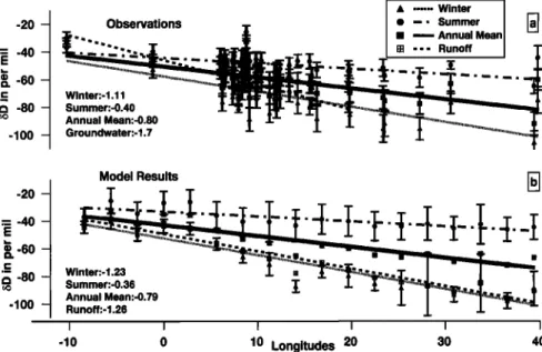
16,880 HOFFMANN ET AL.' WATER ISOTOPES IN THE ECHAM AGCM -20 - E -40 - • -60 - ,... c3 -80 - -lOO - ß ... Winter

Observations

ß -. Summer

...

' t.

[] ''' Runoff

Model

Results

I-b-

]

I I I I I I

-10 0 10 Longitudes 20 30 40

Figure 5. (a, top panel ) IAEA observations

and (b, bottom panel ) ECHAM3 T42-control:

continental

gradient

over Europe

(from West to the East) of 5 180 in precipitation

for summer

(April-September),

winter (October-may)

and the annual

mean. The model

results

(only land

points are considered)

are meridionally

averaged

from 45øN to 55øN and are shown

from 10øW

to 40øE. The isotopic

composition

of groundwater

is taken from Rozanski

e! al. [1982]. Alpine

stations are excluded because of their strong altitude effect.

with a small seasonality in precipitation (<100 cm/yr),

we find a relationship of about 1ø•o per 100 cm an-

nual precipitation. In fact, the model overestimates the

seasonality of the water isotopes in regions dominated

by the amount

effect (T42: 1.5ø•o

and T21: 2.7ø•oper

100cm/yr). This is a particular

problem

in tropical

and

subtropical regions where the model possibly overesti-

mates the height of convection. If strongly depleted va-

por at high altitude is mixed into the convective towers

where the precipitation is formed, systematically very

low 5 values may result without considerably affecting

the total amount of precipitation.

3.3. Surface Hydrology

Considering the coarse spatial resolution of present-

day AGCMs, it is hardly possible to directly evaluate the performance of the model's surface schemes. The

heterogeneity of natural land surfaces makes it diffi-

cult to derive boundary conditions for an AGCM model

grid with a horizontal resolution of some hundred kilo-

meters from observations (i.e., steepness of the orogra-

phy, roughness of the surface, albedo, vegetation types

and coverage, soil types). Given that these difficulties

could be overcome, it is even harder to compare the

simulated large-scale quantities (shortwave and long-

wave back scattering, fluxes of latent and sensible heat,

runoff) with observations which are always biased by

small-scale spatial or temporal variability. An approach

to this problem is the use of a one-dimensional (l-D)

version of the AGCM. Such a 1-D model version in-

cludes the physical parameterization of all AGCM sub-

grid processes adapted to the particular surface con-

ditions of a point observation site. It is forced by ob- served temperature and shortwave radiation. Under the assumption that at least for some hours advective pro-

cesses can be neglected, a direct comparison between

the observed surface fluxes and the simulation results

is possible. Although such efforts were quite successful

[Schulz et al., 1997], we would like to demonstrate here

the potential of stable water isotope simulations to vali-

date AGCM surface schemes on larger scales (temporal

and spatial), without restricting the study on particular

surface conditions.

In Figure 5b the simulated isotopic composition 5D

of precipitation over Europe (T42, meridionally aver-

aged from 45øto 55øN) for summer (April-September)

and winter (October-March) as well as the annual mean

is shown as a function of longitude. The annual mean is influenced to approximately even parts by summer and

winter precipitation. In correspondence to observations

the model simulates no pronounced rainy season over Europe (at the 35 European IAEA stations, 54% of annual precipitation falls in summer compared to 50%

modeled by the ECHAM) which otherwise would domi-

nate the annual isotopic signal. In summer a large frac- tion of precipitation reevaporates from the surface and contributes to subsequent precipitation. Over Europe, evapotranspiration by plants dominates, compared with evaporation from bare soils. As plants do not fraction- ate the vapor transpired by their leaves against the wa- ter taken up by the roots, the isotopic depletion of wa- ter vapor is much weaker under warm conditions with a higher degree of water recycling than under cold con-

HOFFMANN ET AL.: WATER ISOTOPES IN THE ECHAM AGCM 16,881

ditions. This process is an additional feedback mecha-

nism to the temperature effect. In the interior of the

continent it weakens still more the isotopic rainout than

what is inferred from the higher summer temperatures.

The simulated continental gradient of the water isotopes

amounts

to 0.36ø•06D

per deg longitude

eastward

(ob-

served

0.4ø•0 per deg) in summer

and 1.23ø•0

per deg

(observed

1.11 ø•0 per deg) in winter. The model

agrees

fairly well with observations but shows a variability par-

ticularly in the interior of the continent

of up to 20%

higher than is observed.

Rozanski et al. [1982] developed a simple Rayleigh

type model designed to explain the 5 values of Euro-

pean precipitation. They showed a high sensitivity of

the simulated isotopic signal on the reevaporation from

the surface, which in their model is a prescribed quan- tity tuned optimally with respect to observations. In the ECHAM model, the evaporation flux from the sur- face E is an independent quantity calculated from prog- nostic variables. E mainly depends on temperature,

vegetation

coverage

(prescribed

higher than 80% over

Europe), soil wetness, and stability of the planetary

boundary layer. Therefore we conclude that at least

over Europe the underlying assumptions made for the

computation of the evaporation are supported by our isotope simulations. For a more quantitative validation

of the surface processes by the water isotopes a detailed

sensitivity study is necessary which relates changes of

the surface parameters to calculated changes of the con-

tinental isotope gradient. Only such an analysis will re-

veal if the good agreement of the modeled and observed

isotope gradient depends on the seasonally varying con-

tribution of reevaporated water or is just a trivial result

of the temperature effect.

Furthermore, studies investigating the isotopic com-

position of water in plants show a large spatial variabil-

ity [White et al., 1985; White, 1989; Wang and Yakir,

trees with long roots in contact with groundwater take

up water which integrates the isotopic signal over sev- eral months. The simple bucket type surface scheme

of the model averages spatially and temporally strongly

varying conditions at the evaporation sites, at least over

Europe in an approximately correct manner.

The Amazon Basin represents another region where

detailed studies on the relation of the continental effect

and recycling of water have been done [Salati et al.,

1979; Gat and Matsui, 1991; Grootes et al., 1989]. Here

the hydrological cycle runs much faster than over Eu-

rope. Moist air masses are advected by the trade winds

from the tropical

Atlantic

westward

into the basin

and

rainout in convective systems. The amount of water

vapor which reevaporates isotopically unchanged from

the tropical

rain forest

is very

I large throughout

the year.

From the observed mean isotopic gradient of 0.083ø•0

per degree longitude (to the West) it has been estimated

that in the annual mean, about 40% of the advected va- por leaves the basin again in vapor form. This percent-

age undergoes large seasonal variations between 0 and

90% [Grootes et al., 1989]. The ECHAM model also

simulates, compared to Europe, a much weaker spatial

gradient of 0.089øg0 per in the Amazon Basin, indicat-

ing that the model predicts approximately the correct contribution of locally evaporated vapor to the precipi- tation in that region.

Moreover, the water isotopes bear the potential to test also other components of the hydrological cycle over land. The dotted line in Figure 5a (adopted from

Rozanski et al. [1982]) shows a rough estimate of the

mean isotopic composition of European groundwaters

(for the database

see also Rozanski

[1985]). At least in

central Europe it is more influenced by winter precip- itation. Groundwater formation is supposed to domi- nantly take place under winter conditions when the soils are wet and saturated. Moreover, a much smaller part of the precipitation reevaporates during winter. The dotted line in Figure 5b shows the simulated 6D value of the modeled runoff which represents both the di-

rect surface runoff (i.e., rivers) and the water available

for groundwater formation, as represented in ECHAM's

simple surface scheme. The isotopic composition of the ECHAM's runoff is very close to the winter pre- cipitation, indicating that the simulated groundwater recharge mainly takes place in wintertime. This indi- rect inference is confirmed by analyzing the seasonality of the modeled runoff itself. Indeed, 75% of the model's annual runoff in Europe is formed in wintertime.

Rivers are another important component in the global hydrological cycle. They transport back to the ocean all the continental precipitation that is not captured in internal drainage basins such as the Sahara or the Great Salt Lake region in the United States. Studies on the isotopic composition of river water published so far mainly focus on the mixing of different isotope sig-

nals of tributary rivers at their confluence (for exam-

ple, Fritz [1981] discusses observations from the Rhine,

Mackenzie, Mississippi and the Amazon Rivers). Un-

fortunately, systematic measurements over several years

are, at least to the author's knowledge, not yet avail- able. The 6 value of river water is influenced by a num- ber of factors. The most important is the isotopic com- position of precipitation in the catchment area. Other

processes become important for the understanding of

the seasonal cycle of the isotopes in rivers such as the

onset of snowmelting (snow being of course highly de-

pleted), the amount of surface runoff determined by soil

conditions (wet or dry), and reevaporation or evapo-

rative enrichment of river water under warm and dry conditions. From the modeler's point of view the cross- check of the simulated river runoff with the isotopes provides the possibility to test these mechanisms.

AGCM's river runoff into the ocean was already cal- culated in order to fully couple atmospheric and oceanic GCMs [Russell and J.R.Miller, 1990; $ausen e! al.,