The Electric Field and Waves Instruments on the Radiation Belt Storm Probes Mission

HAL Id: insu-01291394

https://hal-insu.archives-ouvertes.fr/insu-01291394

Submitted on 15 May 2020

HAL is a multi-disciplinary open access

archive for the deposit and dissemination of

sci-entific research documents, whether they are

pub-lished or not. The documents may come from

teaching and research institutions in France or

abroad, or from public or private research centers.

L’archive ouverte pluridisciplinaire HAL, est

destinée au dépôt et à la diffusion de documents

scientifiques de niveau recherche, publiés ou non,

émanant des établissements d’enseignement et de

recherche français ou étrangers, des laboratoires

publics ou privés.

Distributed under a Creative Commons Attribution - NonCommercial| 4.0 International

License

The Electric Field and Waves Instruments on the

Radiation Belt Storm Probes Mission

J.R Wygant, J.W. Bonnell, K. Goetz, R. Ergun, F.S. Mozer, S.D. Bale, M.

Ludlam, P. Turin, P.R. Harvey, R. Hochmann, et al.

To cite this version:

J.R Wygant, J.W. Bonnell, K. Goetz, R. Ergun, F.S. Mozer, et al.. The Electric Field and Waves

Instruments on the Radiation Belt Storm Probes Mission. Space Science Reviews, Springer Verlag,

2013, 179 (1), pp.183-220. �10.1007/s11214-013-0013-7�. �insu-01291394�

DOI 10.1007/s11214-013-0013-7

The Electric Field and Waves Instruments

on the Radiation Belt Storm Probes Mission

J.R. Wygant· J.W. Bonnell · K. Goetz · R.E. Ergun · F.S. Mozer · S.D. Bale · M. Ludlam· P. Turin · P.R. Harvey · R. Hochmann · K. Harps · G. Dalton · J. McCauley· W. Rachelson · D. Gordon · B. Donakowski · C. Shultz · C. Smith · M. Diaz-Aguado· J. Fischer · S. Heavner · P. Berg · D.M. Malsapina · M.K. Bolton · M. Hudson· R.J. Strangeway · D.N. Baker · X. Li · J. Albert · J.C. Foster ·

C.C. Chaston· I. Mann · E. Donovan · C.M. Cully · C.A. Cattell · V. Krasnoselskikh · K. Kersten· A. Brenneman · J.B. Tao

Received: 21 February 2013 / Accepted: 22 July 2013 / Published online: 11 October 2013 © The Author(s) 2013. This article is published with open access at Springerlink.com

J.R. Wygant (

B

School of Physics and Astronomy, University of Minnesota, Minneapolis, MN, USA e-mail:wygan001@umn.edu

J.W. Bonnell· F.S. Mozer · S.D. Bale · M. Ludlam · P. Turin · P.R. Harvey · R. Hochmann · K. Harps · G. Dalton· J. McCauley · W. Rachelson · D. Gordon · B. Donakowski · C. Shultz · C. Smith · M. Diaz-Aguado· J. Fischer · S. Heavner · P. Berg · C.C. Chaston · J.B. Tao

Space Sciences Laboratory, University of California, Berkeley, CA, USA F.S. Mozer· S.D. Bale

Department of Physics, University of California, Berkeley, CA, USA R.E. Ergun· D.M. Malsapina · M.K. Bolton · D.N. Baker · X. Li

Laboratory for Atmospheric and Space Physics, University of Colorado, Boulder, CO, USA R.J. Strangeway

IGPP and Department of Earth and Space Sciences, University of California, Los Angeles, CA, USA M. Hudson

Department of Physics and Astronomy, Dartmouth College, Hanover, NH, USA J. Albert

AFGL/RVBX, Kirkland Air Force Base, NM, USA I. Mann

Department of Physics, University of Alberta, Edmonton, Alberta, Canada E. Donovan· C.M. Cully

Department of Physics and Astronomy, University of Calgary, Alberta, Canada J.C. Foster

Haystack Observatory, MIT, Cambridge, MA, USA V. Krasnoselskikh

184 J.R. Wygant et al. Abstract The Electric Fields and Waves (EFW) Instruments on the two Radiation Belt

Storm Probe (RBSP) spacecraft (recently renamed the Van Allen Probes) are designed to measure three dimensional quasi-static and low frequency electric fields and waves associ-ated with the major mechanisms responsible for the acceleration of energetic charged par-ticles in the inner magnetosphere of the Earth. For this measurement, the instrument uses two pairs of spherical double probe sensors at the ends of orthogonal centripetally deployed booms in the spin plane with tip-to-tip separations of 100 meters. The third component of the electric field is measured by two spherical sensors separated by∼15 m, deployed at the ends of two stacer booms oppositely directed along the spin axis of the spacecraft. The instrument provides a continuous stream of measurements over the entire orbit of the low frequency electric field vector at 32 samples/s in a survey mode. This survey mode also includes measurements of spacecraft potential to provide information on thermal electron plasma variations and structure. Survey mode spectral information allows the continuous evaluation of the peak value and spectral power in electric, magnetic and density fluctua-tions from several Hz to 6.5 kHz. On-board cross-spectral data allows the calculation of field-aligned wave Poynting flux along the magnetic field. For higher frequency waveform information, two different programmable burst memories are used with nominal sampling rates of 512 samples/s and 16 k samples/s. The EFW burst modes provide targeted mea-surements over brief time intervals of 3-d electric fields, 3-d wave magnetic fields (from the EMFISIS magnetic search coil sensors), and spacecraft potential. In the burst modes all six sensor-spacecraft potential measurements are telemetered enabling interferometric timing of small-scale plasma structures. In the first burst mode, the instrument stores all or a sub-stantial fraction of the high frequency measurements in a 32 gigabyte burst memory. The sub-intervals to be downloaded are uplinked by ground command after inspection of instru-ment survey data and other information available on the ground. The second burst mode involves autonomous storing and playback of data controlled by flight software algorithms, which assess the “highest quality” events on the basis of instrument measurements and in-formation from other instruments available on orbit. The EFW instrument provides 3-d wave electric field signals with a frequency response up to 400 kHz to the EMFISIS instrument for analysis and telemetry (Kletzing et al. Space Sci. Rev.2013).

Keywords Electric fields· Magnetosphere

1 Introduction

The goal of the Electric Field and Waves (EFW) Investigation on the Radiation Belt Storm Probe (RBSP) mission is to understand the role of electric fields in driving energetic particle acceleration, transport, and loss in the inner magnetosphere of the Earth. The overall EFW instrument development was led by the University of Minnesota under Principal Investiga-tor, John Wygant, and Project Manager, Keith Goetz. The hardware and software develop-ment of the RBSP EFW instrudevelop-ment including the Instrudevelop-ment Data Processing Unit (IDPU) and the spin plane and spin axis boom deployment units was carried out by a team led by John Bonnell at the Space Sciences Laboratory at the University of California, Berkeley. A team at the Laboratory for Atmospheric and Space Physics at the University of Colorado led by Robert Ergun provided a signal processing board for digital filtering and on-board calculation of spectral products.

The EFW instrument provides electric field measurements on each of the two RBSP spacecraft focusing on the frequency range from DC to 256 Hz. In addition, the instrument

has the capability to sample large amplitude 3d electric fields and magnetic fields waves and structures at 16.4 k samples/s in special high rate mode. The frequency range of primary focus from dc to 256 Hz includes measurements of the convection electric field, interactions with interplanetary shocks, electric fields associated with particle injection fronts, Alfven waves, magnetosonic waves, electromagnetic ion cyclotron (EMIC) waves, lower hybrid waves. The candidate structures and waves that have been proposed for the acceleration of different particle populations in the inner magnetosphere span over seven orders of mag-nitude in time and four orders of magmag-nitude in amplitude. The generation of these waves and their ability to accelerate different particle populations is often tied to the dynamics of the inner magnetosphere during geomagnetic storms. During these times, the free energy sources available to drive magnetospheric processes increase by∼2 orders of magnitude (Axford1976) due to encounters powerful interplanetary shocks, coronal mass ejections, and fast-slow streams in the solar wind. During major geomagnetic storms, the plasma pres-sure between 2 REto 6 REis dominated by the development of a hot (20–700 keV) ion ring

current torus surrounding the Earth which is generated by intense convection electric fields that appear deep within the magnetosphere. The spatial configuration of the convection elec-tric fields is modified by the development of powerful ring current pressure gradients in a complex interplay of self-consistent dynamics that ultimately controls the cold plasma den-sity structure, the intenden-sity and configuration of the magnetic field, and the ability of the system to support a wide variety of wave modes. A signature feature of major geomagnetic storms is the erosion of the plasmasphere on the night-side to within 2 REof the Earth in

the equatorial plane. During this massive reconfiguration of the inner magnetosphere, rela-tivistic particle acceleration and loss mechanisms are particularly strong and variable. More than half a dozen different acceleration mechanisms with varying degrees of theoretical and experimental support have been invoked to explain the several order of magnitude increases and decreases in relativistic and near relativistic electrons and energetic ions.

In this section, we present examples of electric field measurements and their limitations from the CRRES spacecraft to illustrate the varied roles of the electric field in the inner mag-netosphere. These data motivated the measurement goals of the RBSP EFW instruments. Next we present recently obtained on-orbit data from the first few months of the RBSP mission that illustrate instrument capabilities. In subsequent sections, we present the mea-surement goals of the instrument, followed by an instrument overview and a more detailed discussion of the instrument subsystems.

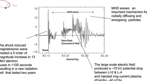
Figure1presents a pass from the CRRES spacecraft through the inner magnetosphere in the equatorial plane during the major geomagnetic storm of March 1991. These data il-lustrate three different energization processes that produced dramatic effects on different particle populations. The three processes are: (1) interplanetary shock induced acceleration; (2) anomalously large enhancements in the convection electric field; and (3) large amplitude ULF waves present throughout the inner magnetosphere. This figure shows an abrupt en-hancement in the electric field of 40 mV/m on the night-side of the Earth near L= 2.4 with a duration of 60 seconds associated with an interplanetary shock induced magnetosonic wave (Wygant et al.1994). It is estimated that the amplitude of the magnetosonic wave on the dayside, where it was directly incident on the inner magnetosphere, was on the or-der of 250 mV/m. Energetic electron measurements on CRRES showed (Blake et al.1992; Blake and Imamoto1992; Vampola and Korth1992) that this structure produced a five order of magnitude enhancement in >13 MeV electrons over a period of <1 minute that evolved into a new radiation belt near 2 REthat lasted over 2 years. The shock induced prompt

ac-celeration of the relativistic electrons was subsequently reproduced in detail by large-scale test particle simulations (Li et al.1993; Hudson et al.1997). Shock induced acceleration of protons was also observed during this event and simulated (Hudson et al.1995).

186 J.R. Wygant et al.

Fig. 1 CRRES measurements during major geomagnetic storm of March 21, 1991 showing interplanetary

shock induced electric fields, the enhancement in the large scale electric field, and ULF waves. Inset figure shows the CRRES orbit with “explosion symbol” indicating position of spacecraft at time of encounter with shock induced magnetosonic wave and tip of red arrow indicating end of plot interval. Text indicates the kinds of energization expected from each structure

Figure1also shows an enhancement in the large-scale dawn-dusk convection electric field from quiet time values of 0.1 mV/m to values of 5–7 mV/m during the main phase of the storm. Measurements of the magnetic field perturbations associated with ring current plasma provide evidence that the plasma was injected by this electric field to a radial dis-tance of∼2 REover a several hour period (Wygant et al.1998; Rowland and Wygant1998).

Radar measurements at ionospheric altitudes also provide evidence for similar storm time enhancements of the large-scale convection electric field at low latitudes (Yeh et al.1991).

Finally, Fig.1shows strong MHD fluctuations of∼10 mV/m lasting almost the entire or-bit that in principle could interact strongly with∼1 MeV electrons stochastically to produce radial diffusion and energization through conservation of the first adiabatic invariant. Alter-natively, the acceleration could proceed through a “coherent” non-linear interaction involv-ing trappinvolv-ing in the quasi-monochromatic large amplitude waves. In order to understand the role of ULF waves in the energization of radiation belt particles, the amplitude of the electric field, its propagation velocity, its azimuthal wave number, and its radial spatial scales must be measured (Hudson et al.2001,2004; Brautigam et al.2005). These properties should be measured as a function of radial position and local time. In addition, the mechanisms responsible for the generation of the waves should be understood. Candidate mechanisms for generating these waves include magnetopause surface perturbations driven by solar wind dynamic pressure variations, reconnection at the front-side magnetopause, large scale shear mode instabilities on the flanks of the magnetopause, the internal free energy in anisotropic ring current ion distribution functions, and stochastic forcing by substorm related electric fields. The existence of the two RBSP spacecraft, upstream solar wind monitors, and the routine presence of the THEMIS spacecraft at larger radial distances will be used to eval-uate the driving forces, the structure of the waves, and to distinguish between competing accelerating mechanisms.

Evidence from CRRES and other spacecraft also has shown that substorm injection fronts propagating inward from the tail can also produce electric fields ranging from 1–40 mV/m for periods of 1 to 5 minutes (Rowland2002; Dai et al.2011; Li et al.1998). These fronts could result in the injection and energization of both ring current ions and high-energy elec-trons (10–700 keV), which are the dominant contribution to the particle energy density and pressure around the Earth during major geomagnetic storms. There is evidence (Ingraham et al.2001) suggesting that intense substorm injection fronts may be able to energize sig-nificant fluxes of electrons up to >1 MeV below L= 4−5 over time scales of minutes. However, our understanding of the efficiency of the mechanism is largely based on CRRES, which only saw one very large storm on the night side of the Earth. In addition, because CR-RES was a single spacecraft, it could not measure the propagation velocity of the injection event or the radial and azimuthal extent of the region of accelerating electric fields.

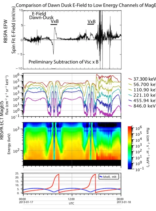
Figure2presents measurements of the dawn-dusk electric field from the EFW instru-ment on RBSP-A and of the energetic electron omni-directional fluxes from the MagEIS instrument during an injection event associated with a small storm on January 17, 2013. The fluctuating electric field is significantly enhanced over the four hour time interval from 18:00 UT to 22:00 UT, often exceeding 10 mV/m. There is also am average positive value of the Ey mgse (or dawn-dusk) electric field component of 1–3 mV/m beginning at 14 UT and lasting about two hours until the spacecraft move earthward to lower l-values. The dc field is seen again on the out bound pass from 18 UT to the end of the day. Thus the electric field is observed nearly continuously as the spacecraft moves from midnight to the morning sector. The total period of enhanced dawn-dusk electric fields is nearly eight hours. This period coincides with a decrease in Dst from 33 at 14:00 UT to−53 at 24:00 indicating an injection of ring current plasma during this period of strong electric fields. While there have been a number of studies of large amplitude convection and ULF electric fields in the tail and on the night side near geosynchronous orbit, to our knowledge, these are the first obser-vations showing that such large fields can be nearly continuously present for many hours. A cursory examination of this and similar time intervals provides evidence for a rich phe-nomenology of magnetic field dipolarizations, plasma-sheet expansions and contractions, encounters with the plasma sheet boundary layers, Alfven waves and other ULF waves, and enhancements in the large scale convection electric field. The second panel of Fig.2 shows line plots of flux from selected MagEIS electron energy channels ranging between 37 keV and 846 keV. The third panel presents color-coded electron fluxes from the MagEIS instrument (Blake et al.this issue) in an energy time spectrogram format. The data from the second and third panel suggest an abrupt injection of <100 keV electrons during the period of the enhanced quasi-static and fluctuating electric field. At the same time, the particles fluxes with energies larger than 100 keV are decreased by about an order of magnitude. This behavior illustrates the complexity of response of different energy particles to electric fields that vary over different spatial and temporal scales. Much detailed analysis remains to unravel the complicated phenomenology revealed by this data set.

The lower values of the electric field, with magnitude less than 1 mV/m seen over the interval from 9:00 to 12:00 UT in Fig.2, indicate the sensitivity of the electric field mea-surement is a fraction of a mV/m. Evaluations of meamea-surements from orbits occurring during especially quiet periods (Kp < 1) indicate the spin-plane electric measurement is sensitive to fields of <0.3 mV/m.

The CRRES spacecraft had only limited capability of making high time resolution burst measurements, so that intense small-scale wave fields that might violate the conservation of the first or second adiabatic invariants within the injection front could not be evaluated. The RBSP EFW electric field measurements along with measurements of the magnetic field

188 J.R. Wygant et al.

Fig. 2 RBSP-A measurements from January 17, 2013 of the (upper panel) dawn-dusk component of the

electric field from the spin plane booms at a spin period cadence (11.5 s). The second panel presents the omni-directional electron energy flux from selected energy channels (37 keV to 846 keV) from the MagEIS instrument. The third panel presents a color-coded omni-directional fluxes in a energy-time spectrogram over the lower energy channels of the MagEIS instrument (MagEIS data courtesy J. Fennell, H. Spence and J.B. Blake). The bottom panel consists of line plots of the spacecraft L-value and Magnetic Local Time (MLT) in units of hours

and energetic particles from other instruments will determine, for the first time, the global spatial structure and time evolution of injection events as they propagate through the inner

magnetosphere. This information is crucial for assessing the ability of diverse structures to accelerate particles of different energies and inject them deep into the inner magnetosphere. At higher frequencies, the EFW instrument will measure electric fields associated with kinetic Alfven waves, lower hybrid waves, ion cyclotron waves, and small-scale discrete structures such as solitary waves. Since CRRES, a number of studies have suggested that whistler mode chorus with amplitudes of 0.1 to several mV/m can be effective in the stochastic energization of electrons over 100 keV to >1 MeV (Roth et al. 1999; Horne and Thorne1998; Albert2000; Summers and Omura2007). It has only been in re-cent years that the possible role of large amplitude small-scale or high frequency waves in the prompt energization and loss of charged particles over broad energy ranges has been ap-preciated. High time resolution electron measurements from SAMPEX (Blake et al.1996; Lorentzen et al.2002) have provided evidence for relativistic microbursts, which consist of abrupt enhancements of relativistic electron precipitation over periods small compared to an electron bounce period. Measurement of bremsstrahlung x-rays due to precipitating high energy electrons have been provided by balloon-borne detectors and have similarly shown that relativistic electrons can be scattered into the loss cone on rapid time scales (Millan et al.2002).

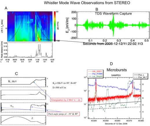
Figure3from Cattell et al. (2008) presents recent STEREO high time resolution burst measurements of very large amplitude (200 mV/m) obliquely propagating whistler mode waves in the inner magnetosphere just outside the plasmapause. Panel A presents a color-coded frequency time spectrogram showing the over all interval of whistler mode power. The lower plot of panel A is the output of a peak detector that provides the peak amplitude each minute of the whistler mode waves. These measurements indicate large amplitude waves at a frequency of ∼0.2fce (the electron cyclotron frequency, plotted in black) are present

for about 30 minutes. Panel B provides a 0.5 second high time resolution measurement of an intense whistler mode pulse from the S/WAVES time domain sampler at a resolu-tion of 35 k samples/s. Panel D provides evidence from SAMPEX of microburst activity on “nearly” conjugate field lines (within 1 hour MLT and 10 minutes) as the STEREO observa-tions. Panel C provides results from a 1-D test particle simulation in which a large amplitude whistler wave is launched along a magnetic field line and interacts with a 1 MeV electron with an initial pitch angle of 30° through a cyclotron resonant interaction. The top panel plots kinetic energy in MeV, the second panel plots the resonance mismatch (see Roth et al. 1999), the third panel plots the equatorial pitch angle, the bottom panel plots the distance along the field line from the equatorial plane in km and the x-axis is time from 0 to 2 sec-onds, with the electron initially at the equatorial plane. The figure shows that the whistler traps the electron and accelerates it up to 4 MeV in about 0.2 seconds (first panel). The wave also causes strong pitch angle scattering (third panel). The results from these simple test particle simulations indicate that large amplitude whistler mode waves may be capable of nonlinear trapping and acceleration of electrons from initial energies of 100 keV to final energies of 2 MeV over broad portions of phase space in fractions of a second (Cattell et al. 2008) in a single interaction. Over 20 one-half second intervals of large amplitude whistler waves were observed by the STEREO spacecraft during one pass associated with a modest substorm. More evidence for intense whistlers was found by Cully et al. (2008) using the THEMIS spacecraft and, by Kellogg et al. (2010) and Wilson et al. (2011) utilizing Wind data. Evidence for an association of the large amplitude whistler waves with microbursts has been provided by Kersten et al. (2011) using roughly simultaneous measurements from the STEREO spacecraft and the low altitude SAMPEX spacecraft and also measurements between WIND and SAMPEX. An understanding of how the waves are generated and their ability to accelerate particles has been limited by the lack of simultaneous high cadence

190 J.R. Wygant et al.

Fig. 3 Wave measurements from STEREO motivating measurements goals of RBPS-EFW. Panel A: Upper

plot is the electric field spectrogram over frequency range from 2 kHz to 100 kHz (Cattell et al.2008) from S/WAVES STEREO spacecraft during pass through inner magnetosphere showing strongly enhanced power in whistler band near L= 3−4 at about 11 UT; Panel A, lower plot is the peak amplitude in electric field associated with enhanced whistler waves measured once per minute by the peak detector. Panel B: High time resolution waveform capture from STEREO showing large (200 mV/m ptp) whistler wave packets from burst recording at time indicated on spectrogram. Panel C: Test particle simulations of imposed whistler wave field of amplitude 300 mV/m interacting with an electron with initial energy 1 MeV. The top plots is the kinetic energy in MeV, the second plot is the resonance mismatch (see Roth et al.1999), the third plot is the equatorial pitch angle, the bottom plot is the distance along the field line from the equatorial plane in km and the x-axis is time from 0 to 2 seconds. The top plot shows the abrupt coherent nonlinear energization of electrons by 2 MeV and the third plot shows the jump in pitch angle through cyclotron resonance during one interaction. Panel D: Near simultaneous (within 10 minutes) low altitude SAMPEX observations of relativistic electron microbursts over same L value extent as STEREO whistler displaced 1 hour in magnetic local time

energetic particle measurements and field measurements on the same spacecraft. The EFW instrument provides unambiguous measurements of the occurrence frequency of large am-plitude waves, as well as their spatial distribution along magnetic field lines, in radial dis-tance, and in local time. The high time resolution particle measurements will be provided on RBSP by the MAGEIS instrument (Blake et al.this issue) and HOPE instrument (Reeves et al.this issue).

The EFW instrument has the capability of measuring, through burst recordings, large am-plitude (requirement <500 mV/m; capability >4 V/m) waves and structures at frequencies up to 16.4 k samples/s and recording them in burst memory. These will be compared to high time resolution measurements of particles by the HOPE and MagEIS instruments on RBSP

and also to measurements of microburst X-rays detected by balloon-borne instrumentation flown during the BARREL campaign (Millanthis issue).

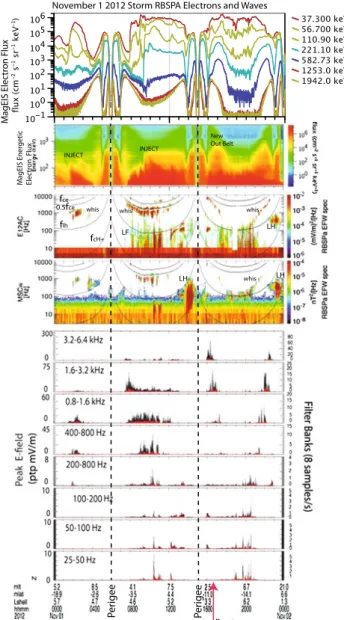
Early measurements from the EFW instruments on RBSP during several major storms illustrate that large amplitude whistler waves routinely have peak values ranging from 10 to >200 mV/m over the entire orbital path outside the plasmasphere during active periods. The incidence of high amplitude whistler waves systematically enhances during major storm periods from apogee at 5.8 Re to radial distances below 3 Re, spanning the position of the outer radiation belts. Figure4presents measurements from the main phase of a geomagnetic storm on November 1, 2012. The top panel shows line plots of flux from selected MagEIS electron energy channels ranging between 37 keV and 1942 keV (Spence et al.this issue; Blake et al.this issue); the second panel presents the omidirectional electron fluxes from the MagEIS in an energy time spectrogram format showing a series of injection events (labeled “INJECT”), the outer radiation belts (“OB”) and the slot region between the outer and inner belts. Notice that during the final orbit the energetic electrons display a complex signature. Near apogee, between 18:00–20:00 UT, the lower energy (36 and 57 keV) electron fluxes near apogee are strongly enhanced over the previous orbit. The higher energy electrons (100 keV to 2 MeV) fluxes decrease relative to those of the previous orbit. This complex behav-ior is the consequence of the interplay between a variety of different acceleration and loss mechanisms, including enhancements in the large-scale convection electric field, changes in the magnetic field configuration, current sheet scattering, magnetopause shadowing, and higher frequency wave activity. Here we emphasize observations of the waves. The next two panels present frequency-time spectrograms of the spectral power in the wave electric and magnetic fields (respectively). The wave magnetic field is measured by the magnetic search coil sensor in the EMFISIS instrument (Kletzing et al.2013) and provided to the EFW instrument via an analog interface. The electric and magnetic spectrograms show that there are enhanced whistler mode waves (labeled “whis”), which extend from near apogee down to radial distances coinciding with the outer radiation belts. Whistler mode chorus is thought to be generated at the magnetic equator and is usually observed in two bands, an up-per band and a lower band centered on fce/2 at the equator. The second orbit during this day

is near the magnetic equator and provides, as expected, the upper and lower band separated by the measured fce/2. However, during the last orbit, which occurs during the main phase

of the storm, the spacecraft is at higher magnetic latitude and the instrument observes only the lower band, and its upper limit frequency is much less than the locally measured fce/2.

This suggests the possibility, subject to further analysis and observations from other time intervals, that the value of the magnetic field at the equator where the chorus is generated is much less than the locally measured magnetic field and thus the frequency of the waves, which (to a good approximation) have group velocities along magnetic field lines and prop-agate to the spacecraft along the field, reflects the equatorial fce/2. These deviations in the

frequency of the whistlers occur almost exclusively during storms when field lines are likely to be especially stretched. They may provide information on the accuracy of magnetic field models and on the adiabatic deceleration of energetic particles, which respond to field line stretching. Such stretching might also enhance magnetopause shadowing and current sheet scattering loss mechanisms. Another possibility, that should be investigated with ray tracing programs, is that the whistler mode waves are not propagating along magnetic field lines, in this especially distorted magnetic field configuration. All these issues need further careful study and are beyond the scope of this initial paper.

Electromagnetic emissions seen in both the electric field and the search coil between the hydrogen gyro-frequency (∼100 Hz) and the lower hybrid frequency (∼1 kHz) are en-hanced at 14:00 UT during an inbound approach to perigee and again at 23:00 UT during

192 J.R. Wygant et al.

Fig. 4 Measurements during the geomagnetic storm on 11/01/2012 from RBSP-A. Top panel is energetic

electron omni-directional flux from selected energy channels from the MagEIS instrument and the second panel is the color-coded omni-directional fluxes in a energy-time spectrogram format from 37 keV to 4 MeV. The third and fourth panels are frequency-time spectrograms showing (third panel) the power in the wave electric field from a pair of E-field booms and (fourth panel) the power in the wave magnetic field from a single search coil magnetometer sensor from the EMFISIS instrument as telemetered through EFW. The subsequent eight panels contain line plots of the peak-to-peak value of the electric field at 8 samples/s in each of a series of frequency bins ranging from 25 Hz to 6.4 kHz in order of decreasing frequency. The vertical scale is variable for each bin and includes the calibrations of instrument frequency response and effective antenna length. The vertical red line coincides with the time of the burst data in the next figure. The wave data from the storm period on 11/01/2012 showing intense average wave power and extra-ordinarily large values of the peak whistler amplitudes over the radial distance from 3 Re to 5.8 Re (apogee). The dark curves superimposed on the wave spectrograms correspond to (in sequence from lowest to highest frequency) the hydrogen ion gyro-frequency, the lower hybrid frequency, one half of the electron gyro-frequency, and the electron gyro-frequency

another inbound approach. These strongly enhanced waves coincide with the position of the “New Outer Belt” which appeared at 14:00 UT. Spacecraft potential measurements (not shown) indicate that these waves are observed inside the plasmasphere. It is worth noting that magnetosonic waves and waves near the lower hybrid frequency inside the plasmas-phere are candidate waves for the stochastic acceleration of electrons between 100 keV and several MeV (Horne and Thorne1998).

Strong electric and magnetic fields are also present at apogee between the ion cyclotron and lower hybrid frequencies. These lower frequency waves (labeled “SS” for “Small Scale”) are in the frequency range of lower hybrid waves, ion cyclotron waves, kinetic Alfven waves, and magnetosonic waves. The bottom set of 8 panels in Fig.4show the peak electric field measurements in selected frequency bins ranging from 20 Hz to 6.4 kHz. These electric field peak detectors are sampled routinely with unprecedented time resolution; each channel is sampled 8 samples/s compared to 1–2 samples per second or once per spin on previous spacecraft electric field instruments. The RBSP sampling is comparable to the time interval between individual wave pulses and allows us to count high amplitude whistler-mode and other wave whistler-mode pulses. These peak measurements will enable assessment of the role of large amplitude whistler waves in the non-linear scattering and energization of energetic electrons and provide context for burst measurements of electric fields (see, for example, burst at time of red arrow shown in Fig.5). In this plot, they reveal that intense whistler waves with amplitudes exceeding 100 mV/m (peak-to-peak) are present before and during periods of enhanced outer belt fluxes and extend over the entire spatial extent of the outer zone radiation belts down to the slot region. These are necessary conditions for the waves to be important in accelerating outer zone energetic electrons.

Routine high-time resolution burst measurements of electric field waveforms from RBSP allow a detailed examination of wave properties. Figure5shows 0.8 seconds of data (from a total burst duration of 5 seconds sampled at 16.4 k samples/second) obtained on the Novem-ber 1, 2012 storm period at 16:20:26 UT (red arrow in Fig.4) from the RBSP-A EFW burst memory. The figure shows packets of large amplitude whistler wave with peak to peak amplitudes exceeding 200 mV/m.

As previously discussed, the structure and dynamics of the plasmasphere are impor-tant for understanding the dynamics of the inner magnetosphere during major geomagnetic storms. The plasmasphere can be strongly eroded during major geomagnetic storms by the action of the large-scale convection electric field. During these times, the plasmapause can move from its quiet time position of >5 Re to within 2 Re. However, there have been few direct experimental comparisons in the outer magnetosphere between the large-scale elec-tric field and the plasmaspheric structure. Information on cold plasma densities is provided on the RBSP mission by tracking the frequency of the upper hybrid line as determined by the EMFISIS instrument and by the measurement of the spacecraft potential by EFW. The EMFISIS determination of density is more accurate than the density estimated from space-craft potential and less subject to uncertainties associated with cold electron temperature effects. The spacecraft potential measurement provides higher time resolution ranging up to 16 samples/s in routine survey mode. Figure6presents a cross calibration over one day and several orbits between density determined the upper hybrid line and that estimated from the EFW spacecraft potential. The plasmaspheric profile is clearly shown in the spacecraft potential measurements and the cold plasmaspheric density determined to better than the 50 % accuracy of the measurement goal.

The two RBSP spacecraft provide measurements at radially and azimuthally separated points deep in the inner magnetosphere allowing, for the first time, the determination of the spatial extent, velocities of propagation, and temporal evolution of large scale electric field

194 J.R. Wygant et al.

Fig. 5 EFW burst recording on 11/01/2012 16:20:26 of high time resolution measurements of two

compo-nents of the electric field in the spin plane of the spacecraft showing a whistler waveform over a period of 0.8 seconds. This burst was triggered by the peak power in the electric field determined by the sum over the five highest frequency bins in the filter banks shown in the previous figure. The time of this burst coincides with the red arrow labeled “burst” at the bottom of Fig.4. EFW bursts also include search coil magnetometer data from the EMFISIS instrument (not shown). The total burst duration was 5 seconds

structures associated with shocks, injection fronts, and MHD waves. The two spacecraft measurements will distinguish between temporal and spatial structures in the hot ring cur-rent plasma and allow the measurement of ring curcur-rent pressure gradients that control the configuration of convective flows. This provides a framework for understanding the abil-ity of different mechanisms to selectively energize different particle populations. The two spacecraft mission will determine the radial and azimuthal extent of the higher frequency wave fields thought to be important in energization and scattering. The amplitude structure, occurrence frequency, polarization, direction of propagation, E/B ratios and local density structure will be investigated in detail.

Previous magnetospheric missions missed many of these effects because the spacecraft orbits were not in the equatorial plane, they had apogees outside the region of interest, and they passed through the inner magnetosphere for only short periods of time often missing the intervals of powerful acceleration. They sometimes were not equipped with the necessary complement of electric field, magnetometer, and particle instruments. The CRRES space-craft, which has provided some of the most interesting measurements in the inner magne-tosphere, took measurements when the monitoring of upstream solar wind conditions was sporadic. There were no solar wind observations of the interplanetary shock or the CME that

Fig. 6 Comparison of spacecraft

potential to the density determined from the upper hybrid line. The top panel is the color-coded spectrogram of the wave electric field over the frequency range from about 10 kHz to above 400 kHz in a frequency vs time format (obtained the EMFISIS instrument). The superimposed dark line is the prediction of the upper-hybrid line based on an empirical fit to the EFW measured spacecraft potential. The bottom panel is the directly measured spacecraft potential measured as the sum of the potential measurement of the individual probes in the spin plane (V1+ V2)/2

drove convective flows and ring current injection for the March 1991 storm or most of the other storms of the CRRES mission. The CRRES electric field instrument had only a small burst memory and a limited capability for high time resolution measurements of electric fields and therefore never saw the large amplitude whistler waves thought to be a major en-ergization candidate. Some of the most important measurements of large amplitude whistler waves came from the WAVES instrument on STEREO and also the WAVES instrument on WIND. The STEREO mission was a two-spacecraft solar wind mission that only orbited through the inner magnetosphere about a half a dozen times on their way out to their respec-tive orbits around the Sun. The observations of numerous large amplitude whistler wave packets were obtained during just one pass during a modest substorm and were not part of the prime science effort of that mission. The WIND spacecraft similarly orbited through the inner magnetosphere only a limited number of times.

Another major NASA asset that will significantly enhance the science return of EFW and other RBSP instruments is the THEMIS spacecraft, which will be able to provide cru-cial information on electric fields and particles at larger radial positions which provides the source population for many of the inner magnetosphere acceleration processes. The EFW team includes Co-Is associated with the electric field experiment on THEMIS. In order to enhance global coverage of the large-scale electric field and provide insight into the iono-spheric effects of major geomagnetic storms, the EFW team has included the Millstone Hill radar, which provides measurements of electric field in the mid-latitude regions. In addition, the EFW team plans to coordinate high time resolution burst electric field measurements with the BARREL investigation (Millanthis issue), which will provide balloon-borne mea-surements of X-rays associated with relativistic electron microbursts.

196 J.R. Wygant et al. 2 EFW Measurement Requirements

In order to measure the electric fields responsible for the acceleration mechanisms described above, the EFW instrument has been designed to meet a series of demanding measurement requirements and goals. The most important requirements driving instrument design are described below. The instrument meets or exceeds these requirements.

• Measure 2-d quasi-static electric fields in the spin plane of the spacecraft at radial dis-tances >3 REto an accuracy of 0.3 mV/m or 10 % of the maximum electric field

ampli-tude, which ever is larger, over a dynamic range of±500 mV/m.

• To provide measurements of the quasi-static electric field component along the shorter spin axis booms to an accuracy of 4 mV/m or 20 % of the maximum electric field magni-tude at radial distances of >3 Re.

• To provide measurements of cold (<30 eV) plasma variations in the plasmasphere over time scales from DC to <1 s with an accuracy of 50 % over a density range from 0.1 to 50 cm−3.

• To provide burst waveform measurements of large amplitude electric fields up to at least 250 Hz with an accuracy of 0.3 mV/m and a range of 500 mV/m at a cadence of 512 sam-ples/s.

• To include measurements of the 3-d wave magnetic field obtained from the EMFISIS instrument in burst recordings (along with the wave electric field measurements described above) up to at least 250 Hz.

• Provide interferometric timing of the propagation of small-scale waves and structures between opposing sensor pairs using burst recordings with a time cadence of up to 16.4 k samples/s.

• Provide spectral and cross-spectral information on the wave electric fields, magnetic fields, and density fluctuations up to 250 Hz.

• Provide the EMFISIS wave instrument with the three measured components of the electric field over the frequency range from 10 Hz to 400 kHz with a noise level of 10−13V2_/m2_Hz

at 1 kHz and 10−17 V2_/m2_{Hz at 100 kHz with a 90 dB dynamic range and a maximum}

signal of 30 mV/m.

3 Overview

3.1 Instrument Design

The design of the RBSP EFW instrument is based on heritage from a long line of dou-ble probe instruments including those on the S3-3 spacecraft (Mozer et al.1979), ISEE-1 (Mozer et al.1973), CRRES (Wygant et al.1992), Viking (Marklund1993), Freja (Mark-lund et al.2004), FAST (Ergun et al.2001), Polar (Harvey et al.1995), the Cluster multi-spacecraft mission (Gustafsson et al.1997), and the THEMIS spacecraft (Bonnell et al. 2008). An extensive discussion of electric field measurements and error sources of this kind of electric field instrument may be found in Bonnell et al. (2008).

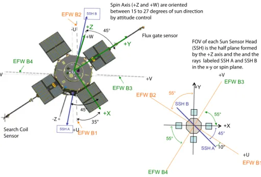
On RBSP the three dimensional electric field is measured using spherical sensors at ends of two orthogonal pairs of centrifugally deployed spin plane booms with tip to tip separa-tions of 100 m and a pair of spin-axis stacer booms with an adjustable tip to tip separation of 12–14 m. A schematic of the spacecraft showing the orientation of the booms is presented in Fig.7. Also shown are the search coil and fluxgate magnetometers. Table1presents in-formation on the relation between the spacecraft coordinate system and the measurement

Fig. 7 Overview picture of RBSP spacecraft showing orientation of EFW spin plane boom sensors, EFW

axial boom sensors, and EMFISIS 3-D Magnetic Search Coil sensors, spacecraft coordinates (xyz) and sensor coordinates (UVW) are indicated. Also shown are the two Sun Sensor Heads (SSH A and B) FOV directions relative to spacecraft coordinates and EFW spin plane booms. Magnetic Search Coil sensors directions and EFW booms are aligned in a common the UVW coordinate system for ease of analysis

Table 1 Boom locations and

telemetry channels relative. To coordinate systems on the spacecraft EMFISIS Science Coordinates (SCM& FGM) S/C Coordinates S/C-ICD Boom# EFW TM Channel +V +X + Y 3 4 +U +X − Y 1 2 −U −X + Y 2 1 −V −X − Y 4 3 +W +Z 6 6 −W −Z 5

directions of the electric field, flux gate magnetometer, and search coils. The three orthogo-nal search coil sensors and the three pairs of electric field probes are aligned with each other to facilitate comparison. Additional images of the spacecraft, coordinate systems, electric and magnetic field sensor booms, and instrument fields of view may be found in Kirby et al. (this issue).

The spacecraft rotates in a right-handed sense about the spacecraft+z axis with a nom-inal spin rate∼5.5 RPM. The spacecraft spin axis is directed between 15 and 27 degrees of the Sun, so that the spin plane booms rotate approximately in the y–z GSE plane. The

198 J.R. Wygant et al.

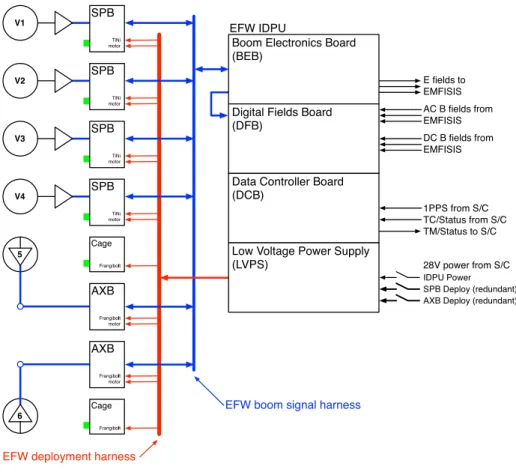
Fig. 8 Block diagram of EFW instrument including Deployment Units, the EFW IDPU, and major interfaces

with the spacecraft and with the EMFISIS instrument. The IDPU block shows major functional subsystems, as well as, signal lines (V1–V6), power lines, diagnostic lines (temperature, boom turns counters), and control lines (motor power, door controls) between the IDPU and the Deployment Units

electric field measurement is most accurate in this plane due to the length of the booms and the nearly uniform illumination of the sensors by the Sun.

A functional block diagram of the EFW instrument is presented in Fig.8. Each EFW instrument consists of an Instrument Data Processing Unit (IDPU) and the six separate boom deployment units. The IDPU consists of a Boom Electronics Board (BEB), a Digital Fields Board (DFB), a Digital Control Board (DCB), and a Low Voltage Power Supply (LVPS) board. The EFW instrument transfers three high frequency analog differential electric field signals to the EMFISIS instrument (Kletzing et al.2013, this issue). From EMFISIS, EFW receives three axis analog search coil AC magnetometer signals as well as the three axis fluxgate DC magnetometer signals. The EMFISIS search coil sensors are aligned with the electric field booms and are measured in the UVW coordinate system as illustrated in Fig.7. Table2presents a summary of the mass, power, and telemetry allocations of the EFW instrument and its major subsystems.

Table 2 EFW mass. power, and

telemetry Mass (kg) Power (W) TM

IDPU 6.4 11 (@30V) 12.0 kbits/s

Shielding 2.2

Spin Plane Booms (×4)

2.04 (8.16) – –

Axial Booms (×2)

3.12 (6.24) – –

Axial boom tube assembly

1.03 – –

Harness 3.36 – –

Total 27.39 10.2 12.0 kbits

4 EFW Design

4.1 Overview of Signal Path, Block Diagram and Science Quantities

This section provides a brief overview of the signal paths and processing through the EFW instrument. A more detailed discussion of the design and functionality appears in subsequent sections.

The potential differences between each of the six spherical sensors and the spacecraft (labeled V1 through V6) are driven by unity gain preamplifiers near the sphere and the signals are sent down their respective boom cables to the Instrument Data Processing Unit (IDPU) where they enter the Boom Electronics Board (BEB). These signals are transferred directly to the Digital Filter Board (DFB) where AC coupled versions of the signals are generated in analog circuitry. The sensor signals from opposing booms are also differenced on the DFB board to provide AC (>10 Hz) and DC coupled versions of the three compo-nents of the electric field. The analog signals are digitized with 16-bit cross-strapped A-D converters on the DFB. Higher frequency (10 Hz–400 kHz) wave electric field signals over the amplitude range (±40 mV/m) are transferred to the EMFISIS wave instrument from the BEB via an analog buffer for wave analysis in that instrument. The digitized sensor and electric field measurements made on the DFB are transferred to the Digital Control Board (DCB) for formatting into Survey and Burst telemetry formats. The DFB provides the three components of the DC electric field from opposite sensors, denoted E12dc, E34dc, E56dc, which are sampled at 32 samples/s and digitally filtered at 10 Hz with a dynamic range of±1V/m and the single ended probe-spacecraft potential measurement (V1 through V6) sampled at 16 samples/s with a dynamic range of±225 volts. These single sensor mea-surements when differenced on the ground can provide electric field meamea-surements with a dynamic range up to 4 V/m. The waveform data are telemetered to the ground continuously over the entire RBSP orbit in a survey mode. The DFB also calculates for inclusion in the survey mode a variety of spectral and filter bank products. These include the complex Fast Fourier Transform (labeled SPEC) of selectable EFW field measurements over a frequency range of 1 Hz to 6.4 kHz. In the default mode, a spectrum is telemetered once every 8 sec-onds and is organized into 64 pseudo-logarithmic frequency bins. The cross spectra between two selected measurements (XSPEC) is also calculated and telemetered to the ground in 64 pseudo-logarithmically spaced frequency bins. The two default measurements used in this calculation are the AC coupled differential electric field measurement from the 1–2 boom pair (E12ac) and the component of the search coil along the spin axis (SCM_W). Continuous

200 J.R. Wygant et al.

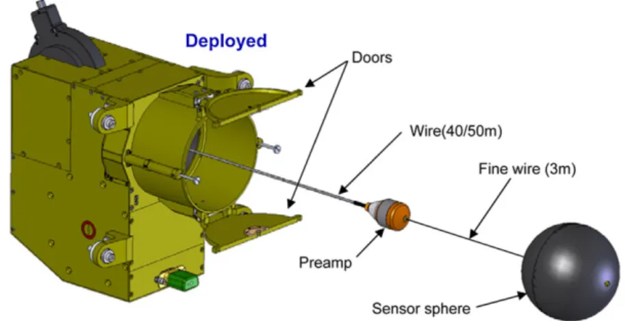
Fig. 9 EFW Spin Plane Boom Deployment Unit in deployed configuration showing deployment unit, cable,

pre-amplifier housing, 3-meter thin wire, and spherical sensor

measurements of rapid variations in average power and peak values of waves, is provided in survey mode for two selectable quantities via a bank of broadband filters. These quantities are denoted FBK_1_av, FBK_1_pk, FBK 2_av, and FBK_2_pk respectively. In the default mode, these broad band filters are sampled at a cadence of 8 times per second in seven pseudo-logarithmically spaced frequency bins from 1 Hz to 6.5 kHz.

High time resolution measurements of waveforms, which cannot be continuously teleme-tered within the allocated EFW telemetry, are provided through two burst modes using two independent burst memories involving different programmable modes of collection and playback controlled by the DCB. The Burst telemetry nominally includes three high fre-quency versions of the differential electric field measurements, the six sensor-spacecraft potential measurements, and the three components of the search coil magnetometer. These modes will be described in more detail in later sections.

4.2 Sensor System and Measurement Accuracy

Spin Plane Sensors The spin plane sensor and cable system is illustrated in Fig.9. The sensor is a conducting metal sphere of radius 4 cm coated with DAG 213 in order to min-imize work function variations over the sphere and from sphere to sphere. In the deployed configuration, the sphere is connected to a high input impedance preamplifier via a thin 3 m long conducting wire. The sensors are current biased to control their floating potential and to minimize their sheath impedance. Theoretical calculations and comparison of measurements from biased and unbiased probes on ISEE-1, CRRES and Polar have shown that current bi-asing can reduce errors due to variations in floating potential by three orders of magnitude. In a manner similar to CRRES, Polar and Cluster, diagnostic sweeps in voltage will be used to determine the optimum value of the bias current. The sheath impedance coupling the elec-tric field sensors to the plasma is adjusted through biasing to be <107_{ohms which is much}

smaller than the input resistance of the PMI OP-15 pre-amplifier input stage (1011_ohms).

Similarly, the capacitive impedance of the 3-meter bare wire portion of the sensor dominates over the input impedance of the OP-15 preamplifier input stage. This sensor design dramat-ically limits both DC and AC voltage divider effects on input signals producing a near unity gain out to high frequencies. The frequency response of the electric field instrument ranges

up to 400 kHz. The OP-15 was used on CRRES and on THEMIS. It is radiation tolerant to 50 krads of total dose and is tantalum shielded to 100 krads to meet the 2-year mission specification. The spin-plane boom cables carry power supply and biasing voltages out to the pre-amplifiers. They carry the sensor voltages measured by the pre-amplifiers back to the main electronics box.

An important error source in the measurement of electric fields is associated with the spurious photocurrents flowing between the spherical sensors and neighboring boom and sensor elements. These photocurrents produce fluctuations in the floating potential of the sphere surface relative to plasma potential. The small surface area of the very thin 3 m long wire connecting the sphere to the pre-amplifier is designed to limit the magnitude of such photo-currents to the sensor. In addition, the flow of photocurrents is controlled by voltage biasing of neighboring surfaces relative to the sphere potential. The biasing is controlled by the DCB microprocessor. The in-board surface called the guard is nominally biased at a constant value of ∼5 volts negative relative to the sphere in order to limit the flux of photoelectrons to the sensor from the nearby cable and the large spacecraft surface. The out-board surface is typically biased∼1 volt negative to limit the outflow from the pre-amplifier housing to the sensor. Precise values will be determined through processor controlled bias sweeps and evaluation of the measurement accuracy at different points along the orbit during commissioning, as well as periodically during the mission.

The fact that the spin axis of the spacecraft is pointed nearly towards the Sun contributes to an especially sensitive electric field measurement in the spin-plane. This orientation re-sults in nearly uniform solar illumination of the spin plane sensors over a spacecraft rota-tion. Consequently, the photocurrent to the spin plane sensors is also nearly constant over a spacecraft rotation. The electric field data will be less accurate when (1) the spacecraft is shadowed by the Earth so that the photo-currents necessary to produce a stable potential reference for the probes are not present, (2) during very brief periods when the thrusters on the spacecraft are firing and the spacecraft is surrounded by a thruster plume, (3) and during periods after attitude maneuvers when the boom cables are oscillating about their equilibrium points.

The spin-axis electric field is about an order of magnitude less accurate than the spin plane measurements since the spin axis booms are shorter by a factor of ∼7 and have a comparatively greater error contribution from asymmetries in the spatial configuration of the spacecraft potential. A new feature of the spin-axis stacer booms on RBSP is that the length of the booms can be controlled such that, after on-orbit calibration, the sensors are positioned on the same equipotential of the spacecraft potential reducing offset errors to the electric field. Thus, the booms are not “popped” outward to a pre-determined length under the spring force of the stacer, but are restrained during deployment by the tension in the cable, which is slowly played out in a controlled fashion by a motor. The motor does not have a retract capability, but does allow the lengths of the two opposing spin axis booms to be independently adjusted.

Accuracy of the measurement along the spin axis booms is affected if the anti-sunward spin-axis boom is partially shadowed by one of the four solar panels as the spacecraft rotates. At these times, because there will be perturbations per spin period, the spin axis electric field component will be calculated from samples obtained from those intervals when the spin axis boom is not shadowed. In addition, spacecraft attitude is controlled by operators to minimize this shadowing by maintaining at least 15 degree offset of the spin axis from sun pointing.

On CRRES, during some of most intense electron injection events, the spacecraft dif-ferentially charged hundreds of volts relative to the plasma. These voltages exceeded the power supply rails of the pre-amplifier electronics and, as a consequence, the electric field

202 J.R. Wygant et al.

instrument sometimes saturated during interesting electron acceleration events. On RBSP, the project instituted a rigorous program of electrostatic cleanliness to insure that the surface of the spacecraft was conducting and that conductive paths tied all major exterior surfaces together including the solar panels and thermal blankets. The electrostatic cleanliness pro-gram was designed to attempt keep spacecraft surfaces electrical equipotentials to within 1 volt and avoid differential charging.

The EFW instrument provides a measurement the spacecraft potential which can be used to estimate of the thermal plasma density in the plasmasphere and identify inter-val of spacecraft charging. The EFW instrument telemeters “single probe potentials”, V1s, V2s, . . . , V6s, which consist of the measured potential differences between individual probe and the spacecraft. The spacecraft potential is calculated on the ground by summing the single probe potentials from sensors on opposite sides of the spacecraft. This sum re-moves the differential electric signal due associated convection, waves, and other ambient plasma processes. In lower density cold plasmas (<100 cm−3), the spacecraft potential rel-ative to the ambient plasma is primarily determined by the balance between photoemission associated with solar illumination and the thermal current associated with thermal electrons in the plasma. The current-biased probes provide a stable reference (within 1–2 volts of plasma potential) for the measurement of the spacecraft potential relative to the ambient plasma. Interpretation of the spacecraft potential in terms of the properties of the thermal electron plasma must include the fact that the spacecraft is typically in the Langmuir probe “focusing regime” (Pedersen1995; Pedersen et al.2008). In these circumstances the space-craft potential scales as the logarithm of the electron density with a small contribution from temperature effects. The spacecraft potential is typically calibrated periodically against other measures of plasma density. As discussed in the Introduction, Fig.6presents a calibration of the spacecraft potential versus density as determined from measurements of the upper hybrid frequency by the EMFISIS instrument (Kletzing et al.2013) over the density range from 1 to 10−3 during one orbit. The spacecraft potential measurements provide a higher time resolution (DC—100 Hz), but less accurate, measurement of the density and thermal plasma structure than the one obtained from the upper hybrid frequency measurement. The spacecraft potential algorithm for calculating density is inaccurate during intervals of neg-ative spacecraft charging induced by very strong fluxes of 10 eV to 1 keV electrons near apogee. Periods of strong spacecraft charging may be identified by comparing the space-craft potential to the HOPE measurement of H+ and O+ over the 10 eV to 5 keV range (Reeves et al.this issue).

Sensor Frequency Response The frequency response of the spin-plane sensor system is governed by the properties of the plasma sheath around the sensors and by the ability of the preamplifier to drive the long 50-meter cables. The source impedance of the plasma sheath surrounding the sensor forms a voltage divider with the input impedance of the preamplifier system. The switch from resistive to capacitive coupling is associated with a roll-off in frequency response from unity near DC to 0.6 at ∼100 Hz. A second higher frequency roll-off in the sensor/cable system occurs as a consequence of the capacitive loading of the preamplifier by the long spin-plane cables. This occurs near 300–400 kHz and defines the upper end of the frequency response for the signals sent to the EMFISIS instrument.

Figure10presents plots of the gain and phase shift of the spin plane and spin axis boom pre-amplifier system and cables at the entrance to the EFW IDPU. Note that the spin axis booms have a higher frequency response as a consequence of the decreased attenuation due to the lower capacitance of the shorter spin axis boom. Additional phase shifts for these measurements are associated with the 5 pole Bessel anti-aliasing filters. For Bessel filters

Fig. 10 Panel A. Calculated (for

low density plasma) SPB sensor frequency response (including phase shift) of signals input to spherical sensors and output at entry to IDPU. Panel B: Same as Panel A for spin axis sensor. The first vertical green dotted line (near 8.2 kHz) indicates the highest frequency signal processed by the EFW instrument. The second dotted line at higher frequency indicates the required upper frequency of the signal passed to the EMFISIS wave instrument

Table 3 Time delay due to FIR

5 pole Bessel filters Sampling rate Delay (ms) Sampling rate Delay (ms)

1 6007.446 256 30.884 2 3007.446 512 19.165 4 1507.446 1024 13.306 8 757.446 2048 10.376 16 382.446 4096 8.911 32 194.946 8192 8.179 64 101.196 16384 7.813 128 54.321

the phase shift is linear as a function of frequency. For time domain signals this results in a constant time delay for a given roll-off frequency. Table3provides the time delays for different anti-aliasing frequencies for the 5 poles Bessel filters appropriate for all quantities in the burst and survey data.

On-orbit Calibration and Analysis of the Electric Field Measurement Calibrations of the electric field instrument can be provided in several ways. During quiet times when geophys-ical electric fields are small, the electric field measurement should approach E= −Vsc× B

where Vscis the spacecraft velocity relative to the rest frame of the Earth and B is the

mea-sured magnetic field. For electric fields that are constant over a spin period, the meamea-sured signal from orthogonal booms pairs should be 90 degrees out of phase and scale in mag-nitude with 100 m boom lengths. During periods of strong flows in the near Earth plasma sheet, the velocity moments, VP, from the HOPE plasma instrument can be used to estimate

E= −VP× B.

Historically it has been found that the most accurate quasi-static electric field determina-tions are provided by least-squares spin-fits to the electric field measured by the spin plane

204 J.R. Wygant et al.

sensors in the rotating frame of the spacecraft. In the rotating system, a constant electric field in inertial space appears as a sinusoidal signal. This fit determines the optimum values of the amplitude and phase of this sinusoidal signal, determining the magnitude and direction of the electric field projected into the spin plane. Such spin fits are especially accurate because they use the large number (484) of measurement points gathered over one spin period and because they remove work function voltage differences between the probes and other errors which appear as constant offsets to the sinusoid. After one fit, the fit may be further opti-mized by removing noise points far from the fit value (i.e. more than 2 standard deviations) and repeating the process as needed to obtained the desired accuracy. Perturbations to the sinusoidal electric field signal observed by the rotating sensors due to angle dependent spu-rious photo-currents or wake effects can removed by selectively masking data points over those rotation angles most susceptible to the perturbations.

Analysis of data from the CRRES spacecraft, which also had a sun-pointing spin axis, shows that the dominant error source for the quasi-static spin plane electric field is typically due to the effect of attitude uncertainties in the Lorentz transformation from the spacecraft frame to the inertial frame of the Earth. The attitude uncertainty of <30_{will allow EFW to}

meet or exceed the spin-plane boom measurement sensitivity requirement above 3 REradial

distance (either of 0.3 mV/m or 10 % of the amplitude of the electric field, which ever is larger). The anticipated Spin plane electric field sensitivity after spin fits and other ground analysis efforts is expected to be 0.1 mV/m (or 10 % of the amplitude) based on CRRES measurements (Rowland and Wygant1998).

Spin Axis Electric Field Measurement The spin axis measurement is especially accurate for higher frequency wave measurements (>100 Hz to 400 kHz) where it provides for a full three-dimensional electric field measurement. However, for quasi-static and low frequency measurements, the measurement is less accurate than the spin plane booms since the spin axis booms provide a shorter measurement baseline. In addition, the spin axis sensors are closer to the spacecraft and sample a larger fraction of the spacecraft charging structure es-pecially at apogee where the Debye length is larger than the spacecraft dimensions and the charging structure has a slower fall-off with radial distance. Since this structure is asymmet-ric with respect to the Earth–Sun line, a portion of this charging structure appears as a differ-ential signal in the low frequency electric field. These asymmetric contributions to the spin axis measurement are partially mitigated on RBSP, since the lengths of the individual spin axis booms may be incrementally adjusted (outward only) during on-orbit calibrations to re-move the contribution from the spacecraft potential to the electric field. Finally, the spin axis booms may be shadowed by solar panels, which rotate and intermittently shadow the anti-sunward boom varying the photoemission and potentials of booms surfaces. This shadowing can produce periodic spikes repeating at the spin period lasting <1/16 second, which must be removed from the data. This photoemission variability is strongest for the anti-sunward spin-axis boom when the spin axis of the spacecraft points directly at the Sun. This shadow-ing near the electric sensors is mitigated on RBSP through on-orbit attitude maneuvers that control the angle between the spin axis of the spacecraft and the Earth sun-line so that it is al-ways larger than 15 degrees. Measurement of the quasi-static spin-axis electric field requires extensive ground analysis and validation. The quasi-static spin axis electric field measure-ment is most useful for large electric fields associated with ULF waves, shocks, and injection events. In addition, it is designed to provide useful information on the structure of the large-scale convection electric field during major geomagnetic storms when the field is especially strong and penetrates to lower L-value, and higher plasma densities (Wygant et al.1998; Rowland and Wygant1998). It is complemented when possible by the derivation of the spin

axis electric field from the measurement of the two spin plane components of the electric field and the full three dimensional magnetic field measurement (from EMFISIS) and the constraint that (for large scale slowly varying fields) E• B = 0.

IDPU Electronics: Boom Electronics Board The signals from the six electric field sensors enter the IDPU onto the Boom Electronics Board (BEB). At this point, the DC signal has a gain of near unity and a dynamic range of∼225 volts. The sensor electric field signal is transferred to the Digital Filter Board (DFB) for signal processing and A-D conversion. Signals from opposing booms are subtracted and sent as buffered wave electric field signals with a frequency response up to 400 kHz to the EMFISIS instrument. The required noise level of the signal to the EMFISIS instrument at the output of this buffer is 10−14V2_/m2_Hz

at 1 kHz and 10−17V2_/m2_{Hz at 100 kHz. This was verified at EFW instrument level testing}

and also during interface testing with the EMFISIS instrument itself. The required minimum dynamic range is±30 mV/m. This value is met and exceeded by the actual dynamic range of∼40 mV/m.

One of the principle functions of the BEB is to generate and transfer the different control voltages that are used for current biasing of the probe and to control the potential of surfaces near the sensors. These signals are transferred to each of the six boom deployment units and then out via wires in the boom cables to each of the sensors. These bias control circuits consist of the current bias circuit, the usher bias circuit, and the guard bias circuit. Each of the sensors is independently controlled by a set of bias circuits.

The current bias circuitry results in the injection of a microprocessor-controlled bias current from the sensor surface into the plasma to control the sensor floating potential and the plasma sensor-sheath resistance. This is achieved by setting the operational point on the current-voltage curve of the sensor/plasma sheath. In low-density plasmas, the bias current is generally adjusted to be a significant fraction of the total photocurrent to the probe. The injected bias current may be adjusted over a range between ±500 nA to an accuracy of 0.2 % by the bias circuitry. The bias circuit has a high frequency roll-off (6 dB) at about 300 Hz. The optimum bias current will be determined by on-orbit bias sweeps during the commissioning phase and also at a lesser cadence throughout the mission. Depending on on-orbit calibration results, the bias current may have different values in the low-density plasma near apogee and in the higher density plasma deep within the plasmasphere.

The usher and guard bias circuits generate voltages that equal the sum of a sphere output plus a microprocessor-controlled voltage offset. The roll-off for the usher signal is 300 Hz and that for the guard circuit is 100 Hz. These circuits control the perturbing sensor-boom photocurrents over the frequency range from DC to somewhat less than 100 Hz where the sensor-plasma sheath impedance is resistive. The usher and guard voltages are transferred via the boom cable to their respective conductive control surfaces on the preamplifier sensor housing. Thus, the potential of these control surfaces relative to the sensor are a constant microprocessor-controlled value. The voltages may be adjusted to a constant value over a range of ±40 volts with a 16-bit DAC. The usher and guard bias potentials will be opti-mized during the commissioning phase and periodically throughout the mission. Typical values range between zero and several times the photoelectron e-folding energy or∼5 volts. Typically, once adjusted to their optimum values, the guard and usher voltages remain con-stant for months to years. The commanded values of the bias, guard, and usher voltages are included in EFW housekeeping telemetry, as are the parameters of the bias sweeps. Search Coil Signals The three components of the wave magnetic field from the EMFISIS search coils (Kletzing et al. 2013) are provided to the EFW instrument via analog lines

206 J.R. Wygant et al.

Fig. 11 Magnetic Search Coil gain and phase frequency response through EMFISIS search coil sensors to

EFW telemetry from 2 Hz to 7 kHz. The different colored dots on the phase curve correspond to different signal generator modes driving the stimulus coils

where they are digitized along with the electric field signals. The EFW instrument science measurements focus primarily on the lower frequency (<250 Hz) portion of the wave signal. The maximum response for the EFW search coil signal is at about 100 Hz but on-orbit measurements indicate that large amplitude waves can be detected in the >2 kHz range. Search coil data is incorporated into EFW spectral products and also burst data collections. The gain (left hand label) and phase (right hand label) responses of the search coil were calibrated relative to the electric field signals during bench tests and also on the spacecraft. The results of these calibrations are shown in Fig.11. The blue and red traces of the phase response simply refer to the nature of the signal from the signal generator that provided the spectral power for optimum calibration. A sinusoidal signal was used at low frequency (blue) and a broad band “white noise” signal was used for high frequency calibration (red). 4.3 Digital Filter Board

The Digital Filter Board (DFB) and associated firmware was designed, fabricated, and tested by a team from the Laboratory for Atmospheric and Space Physics (LASP) at the University of Colorado led by Robert Ergun. The digital filter board is responsible for analog processing of sensor signals, A-D conversion, and anti-aliasing, as well as onboard calculation of a variety of spectral and cross-spectral products.

Time Domain measurements As indicated by Fig.8diagram, and as previously discussed, the analog signals from each of the six spheres are passed to the DFB where the signals from