Multi-model data fusion for river flow forecasting: an evaluation of six alternative methods based on two contrasting catchments

HAL Id: hal-00304716

https://hal.archives-ouvertes.fr/hal-00304716

HAL is a multi-disciplinary open access archive for the deposit and dissemination of sci-entific research documents, whether they are pub-lished or not. The documents may come from teaching and research institutions in France or abroad, or from public or private research centers.

L’archive ouverte pluridisciplinaire HAL, est destinée au dépôt et à la diffusion de documents scientifiques de niveau recherche, publiés ou non, émanant des établissements d’enseignement et de recherche français ou étrangers, des laboratoires publics ou privés.

evaluation of six alternative methods based on two

contrasting catchments

R. J. Abrahart, L. See

To cite this version:

R. J. Abrahart, L. See. Multi-model data fusion for river flow forecasting: an evaluation of six alternative methods based on two contrasting catchments. Hydrology and Earth System Sciences Discussions, European Geosciences Union, 2002, 6 (4), pp.655-670. �hal-00304716�

Multi-model data fusion for river flow forecasting: an evaluation of

six alternative methods based on two contrasting catchments

Robert J. Abrahart

_{and Linda See}

Email for corresponding author: bob.abrahart@nottingham.ac.uk

Abstract

This paper evaluates six published data fusion strategies for hydrological forecasting based on two contrasting catchments: the River Ouse and the Upper River Wye. The input level and discharge estimates for each river comprised a mixed set of single model forecasts. Data fusion was performed using: arithmetic-averaging, a probabilistic method in which the best model from the last time step is used to generate the current forecast, two different neural network operations and two different soft computing methodologies. The results from this investigation are compared and contrasted using statistical and graphical evaluation. Each location demonstrated several options and potential advantages for using data fusion tools to construct superior estimates of hydrological forecast. Fusion operations were better in overall terms in comparison to their individual modelling counterparts and two clear winners emerged. Indeed, the six different mechanisms on test revealed unequal aptitudes for fixing different categories of problematic catchment behaviour and, in such cases, the best method(s) were a good deal better than their closest rival(s). Neural network fusion of differenced data provided the best solution for a stable regime (with neural network fusion of original data being somewhat similar) — whereas a fuzzified probabilistic mechanism produced a superior output in a more volatile environment. The need for a data fusion research agenda within the hydrological sciences is discussed and some initial suggestions are presented.

Keywords: data fusion, fuzzy logic, neural network, hydrological modelling

Introduction

The application of modern digital technologies and computer science techniques to catchment modelling is said to have facilitated a virtual revolution (Singh, 1995). Moreover, the increased potential for rapid application development has created an associated plethora of hydrological models that possess different levels of complexities and sophistication. Modern software solutions, in consequence, offer a vast and diverse range of alternative modelling opportunities; these extend from the application of lumped empirical black-box estimators, to ultra-complex mechanistic simulators that seek to replicate distributed processes throughout a catchment. The downside to this expansion is that each model was designed to fulfill a particular set of scientific aims, or management objectives, so that no single model has the power to provide a superior level of skill across all catchments or under all circumstances.

For operational purposes — such as real-time flood forecasting — a particular model will often be selected from a number of competing solutions. This selection process is based on an assorted collection of personal preferences, such as trust and understanding, or the amount of time and effort that is needed to develop trained and experienced operators. The cost of the licence for a particular model can also be crucial since some software packages are expensive whilst other solutions are to all intents and purposes free of charge. Each end-user will, in addition, need to consider items such as: does this model provide an accurate response; is this model a traditional mechanism based on standard concepts; to what extent will this model be difficult to learn or to put into practice; and, last but not least, to what extent does this model match the available data and particular objective(s) of the catchment modelling requirement(s). Moreover, although each forecaster (active output producer) or decision

maker (passive output consumer) might use a single substantive model to do the bulk of their work, more often than not a simpler tool will be used for simultaneous independent backup and support. The dangers of total reliance upon a single modelling solution and the serious repercussions of short-term failure, which arise from the fact that a single tool cannot provide the best output under all circumstances, are thus diminished.

Shamseldin et al. (1997) and Xiong et al. (2001) recognized the existence of operational dualities and provided theoretical and empirical justification for a multi-model approach. No single multi-model is perfect and will at best describe one or more particular stages, phases or mechanisms of the rainfall-runoff process: so the prudent amalgamation of several discharge estimates obtained from different models can be expected to provide a more comprehensive and accurate representation of catchment response, in comparison to each individual model that is used to build a particular combination. It is possible to perform non-complex combinations, for example to switch between different single modelling solutions at each time step (e.g. crisp probabilistic method of See and Openshaw, 2000), to switch between different single modelling solutions at different levels of discharge (e.g. range-dependent method of Hu et al., 2001), or to develop error forecasting mechanisms that can be used for real time output updating purposes (Serban and Askew, 1991; Shamseldin and O’Connor, 2001). The alternative to simple switching or updating is to implement a linear or non-linear weighted combination: different forecasts obtained from a diverse set of models can be amalgamated, in some optimal manner, which seeks to exploit the inherent benefits of each individual solution. The problem of radical errors should thus be lessened but, if all models drift, then so too will their combined response. This concept of combining forecasts from different models or methods is not original and applications have been reported in a diverse set of subjects ranging from management science to weather forecasting (Clemen, 1989). Moreover, commensurate with recent technological advances, this area of research has evolved into a specialist field of activities termed ‘data fusion’. The scope of applications has also been extended to include a wealth of alternative operations that stretch from ocean surveillance and target recognition to legal enforcement and medical diagnosis (Hall, 1992).

Data fusion

Modern developments in data fusion offer a formal framework that can be used to perform an alliance of data through the provision of concepts, methods, means and tools.

The inspiration behind data fusion has two separate, but not exclusive, objectives:

z to produce synergistic gains, and

z to obtain information that cannot otherwise be obtained

or obtained with the same qualities.

Fusion is often a mix of recognised procedures (e.g. statistical inference, neural networks, belief-based methods or rule-based reasoning (Hall and Llinas, 1997)) that are applied using either (i) modular strategies in which different models are developed to perform different modelling operations and then coupled together or (ii) ensemble strategies in which different models are developed to perform similar modelling operations and their outputs merged, e.g. stacking, boosting or bagging (Sharkey, 1999). The implementation of fusion operations can involve serial, parallel or mixed strategies of data and decision combination. Serial strategies might include items such as: (i) simple pre-processing or post-processing operations in which the output from one model is passed into another; (ii) real-time updating in which observed values are used to correct simulated values (Shamseldin and O’Connor, 2001); or (iii) more complex situations, in which additional variables and the latest observations are used to predict the local error at a point of interest that is then superimposed onto a global simulation or output forecast (Babovic et al., 2001). Parallel strategies include the basic merger of hard and soft data (McKenna and Poeter, 1995) and the complex multifaceted amalgamation of simultaneous outputs, produced using alternative methodologies or rival mechanisms, in the manner of: (i) estimation and addition of residuals; (ii) building modular assemblies of expert sub-units (Zhang and Govindaraju, 2000); (iii) performing weighted combination of individual forecasters (Shamseldin

et al., 1997); or (iv) bootstrapping operations (Srinivas and

Srinivasan, 2000, 2001). The fusion process is not constrained and could encompass the amalgamation of original information to produce an output, or both original and processed information can be fused together to construct more useful outputs, which, perforce, includes decision-making procedures and control related activities. Data fusion can also be used to perform more complicated feature-based or decision-based amalgamations, working on an assorted mix of different sorts of input material to produce a numerical output, a feature output or a higher-level decision. In a strict sense, data fusion would involve using data of different natures that had originated from different sources. It could, for instance, entail working with various different sets of data, collected from several different types of sensor, in association with factual material held as a set of rules

within a relational database or stored as tabular information within a spreadsheet. However, fusion can also be performed on the output from models developed under different methodologies such as forecasting or simulation, or on the output from similar models that contain important differences in terms of structure or input. The goal of amalgamation is to capture and exploit the strengths of each individual approach and, through the process of construction, to build a better final product. This process can also be used to eliminate, or at least to diminish, the worst predictions or greatest errors that exist within each individual single model forecast. The nature of the modelling inputs and outputs will also influence the decision on an appropriate algorithm to match the problem situation. If the inputs and outputs are of a similar form and nature then some kind of weighted, or non-weighted, mathematical average could be computed. But the exact same method cannot be applied to the amalgamation of different types of information such as in the case of using size and speed to determine the likelihood that a moving object is a hostile aircraft.

There is a plethora of different data fusion possibilities and the associated concept of holistic estimation is still under development on a worldwide basis. Each implementation should nevertheless: (i) attempt to capture the full information content of the component data and (ii) endeavour to account for the uncertain relationship between input data and either desired information or end product. The most popular tools in the data fusion toolbox include:

z low-level signal processing procedures e.g. Weighted

Average or Kalman Filter

z traditional statistical methodologies e.g. Least Squares

Estimation or Bayesian Inference

z decision-making techniques e.g. Case-Based Reasoning

or Dempster-Shafer Belief Model

z artificial intelligence technologies e.g. Fuzzy Logic,

Neural Networks or Expert Systems

For a comprehensive discussion on the different algorithms and strategies involved the reader is referred to published material: Abidi and Gonzalez (1992); Brooks and Iyengar (1998); Crowley and Demazeau (1993); Hall and Llinas (1997); Joshi and Sanderson (1999); Kokar and Kim (1993); Luo and Kay (1989). The modelling methods that are addressed in this specific investigation are orientated towards a consideration of artificial intelligence technologies. Earlier research indicates that such tools can provide a fast and cost efficient solution to various complex hydrological modelling tasks — with particular benefits to be gained in the construction of time-series forecasters and

in data fusion operations.

Much of the literature on multi-source information fusion has adopted the tacit assumption that fusion will in all cases impart a better result since using more information to establish an answer should help and not hinder (Dasarathy, 2001). However, recent investigations suggest that various assumed advantages or improvements are not automatic, such that it is possible to construct a parametric definition of the benefits domain (Dasarathy, 1996, 1998, 2000). The question of confidence and trust models is therefore important; black-box implementation of smart or automated mechanisms can produce a ‘fear of the unknown’, wherein the original degree of faith expressed in one or more tried and tested models, is either lost or swamped during the fusion process. To address such concerns would require the formulation and construction of efficient and robust domain-based measures of fusion performance and fusion effectiveness — but the development of pertinent metrics with respect to hydrological modelling is still awaited. This area of research has in fact received limited attention, relative to its overall importance, although some attempts at quantitative estimation of the fusion benefit (or lack thereof) can be found in other domains of scientific investigation (Dasarathy and Townsend, 1999; Xydeas and Petrovic, 2000; Ulug and McCullough, 2000). There has also been an attempt to represent the effectiveness of the fusion process itself – as opposed to the effectiveness of the fusion operation in terms of a correct answer. FAME (Fusion Algorithm Measure of Effectiveness) (Dasarathy, 1999) is the ratio of the performance of a fusion operation to the theoretical performance of an ideal fusion model — in which the latter is a theoretical process that generates the correct response if at least one of the inputs is correct.

The implementation of fusion mechanisms has also encountered several operational quandaries since there are no solid rules to assist in the design and selection of each critical element: architectures; algorithms; inputs and outputs. For example is it better to exploit inputs that are dependent upon each other (cooperation approach); to develop a more complete model (complement approach); or to reduce uncertainties (competition approach)? Fusion can also be a complicated process and the potential gains must be assessed in terms of working overheads with respect to time and effort or cost. To perform real time data fusion will put an additional drain on precious resources and such costs will be commensurate with the need to develop and administer more complex modelling solutions. To this deficit must be added the operational needs and demands of servicing numerous individual models — which must be run on a concurrent basis — to generate numerous streams of redundant output. However, the construction and fusion

of several dedicated neural network forecasters will still take a lot less time and effort than the development of a more complex process-based model. Further related difficulties arise from the fact that there is at present no upper limit on the amount of information that should be entered into a fusion process or established method to determine whether or not improved access to alternative sources of data would be advantageous. Erroneous data can also be awkward or challenging. There is a pressing need to develop improved methods of conflict resolution, perhaps based on specified conditional probabilities, that can be used to lessen the impact of dubious material — since poor input could have a large influence

Previously reported exploration and testing of multi-model data fusion operations within the hydrological sciences is limited in number and extent. Earlier research has involved proof-of-concept assessment and comparison of (i) neural network and soft computing solutions against (ii) means, medians and weighted-averages (Shamseldin et al., 1997; See and Openshaw, 2000; See and Abrahart, 2001; Xiong

et al., 2001). But neural network and soft computing

approaches are at opposite ends of the modelling spectrum in terms of theoretical underpinnings and substantiation of end products. Each approach will possess its own specific set of merits and shortcomings — although in broad terms the two methodologies do in fact complement one another. So, if one method is not successful, then the converse approach might do quite well. Neural network solutions can be used to provide a non-linear outcome in which nothing is assumed or enforced, which is of particular benefit when relationships are difficult to determine, or in situations where fixed and explicit rules are neither relevant nor desired attributes of the mechanism to be modelled. Other potential benefits would include strong ‘fault tolerant’ (model will still operate in spite of both planned and unplanned errors or disruptions to the input data set) and ‘graceful degradation’ (model will continue to operate in problematic situations at a reduced level of service rather than suffer total failure) characteristics — such that acceptable solutions can be developed and run on incomplete, imprecise or noise-ridden data. Soft computing solutions can be used to provide a non-linear alliance of linguistic variables; this method thus offers good opportunities to build upon existing hydrological insight and understanding, through the encapsulation of expert opinion and established science, whilst at the same time providing a transparent solution that can be understood. There are strong indications in the literature that high-tech multi-model data fusion can be used to produce forecasting outputs that are more accurate than (i) individual models or (ii) simple arithmetic operations and weighted statistical functions (Shamseldin et al., 1997; Abrahart and

See, 1999; See and Abrahart, 2001; Xiong et al., 2001). Past investigations also suggest that further research is needed to provide an improved understanding of the hydrological benefits that can be obtained from data fusion operations, for the identification of potential problems or pitfalls with respect to the implementation of different reported mechanisms or strategies, and on the outcome of different data fusion applications in different environments or under different hydrological conditions (Abrahart and See, 1999; See and Abrahart, 2001). To address such matters, this paper draws together six previous data fusion strategies that were applied to a stable river regime and applies an identical set of techniques to a smaller and much flashier catchment. Two fusion benchmarks were first computed using: (i) arithmetic-averaging to produce a mean; and (ii) a probabilistic method in which the best model from the last time step is used to generate the current forecast. Two neural network fusions and two soft computing fusions were then developed and compared against the benchmark products in terms of forecasting skill. The individual tools that created the multi-model input data are not assessed in this paper and no claim is made of such items being optimal solutions for either of the two test catchments. Indeed, there is little doubt that better models could have been developed using alternative solutions or more powerful software packages but, in this instance, the potential benefits of adopting a multi-model approach are the main concern. For practical reasons and demonstration purposes, it is also important to work with single modelling solutions that have different degrees of imperfection which then provide associated opportunities for correction or improvement.

Experimental design

HYDROLOGICAL ENVIRONMENT

This analysis of opposing methods and contrasting catchments is based on a collection of single modelling solutions that were developed for: (a) Skelton on the River Ouse in Northern England: this paper draws together and puts into context two separate reported investigations (See and Openshaw, 2000; See and Abrahart, 2001) and for (b) Cefn Brwyn on the Upper River Wye in Central Wales — a much smaller catchment, with much flashier hydrological characteristics, that offers a useful comparison for this assessment of different methods under different environmental conditions (Fig. 1).

The Ouse catchment of 3286 km2 _{contains an assorted}

mix of urban and rural land uses. This catchment exhibits a large amount of natural variation, ranging from dissected uplands in the west that experience substantial precipitation,

to cultivated lowlands in the east which receive more equitable rainfall. More detailed physiographic and hydrographic information can be found in Jarvie et al. (1997) and Law et al. (1997). Fusion was performed on level forecasts for the gauging station at Skelton. This station is located downstream, far from the headwaters, and the river at this point possesses a stable regime. The adoption of a six-hour-ahead forecasting horizon with respect to individual models and data fusion solutions presented a reasonable challenge to the hydrological modeller. Each set of single model forecasts used in the fusion operation comprised a six-hour-ahead prediction for the period 1989– 92. The four individual data streams to be fused comprised forecasts taken from past reported applications; a hybrid neural network forecaster [IDV-SK1], a rule-based fuzzy logic forecaster [IDV-SK2], an autoregressive moving average time series forecaster [IDV-SK3] and persistence [IDV-SK4]. Further specifics on the development of each single model can be found in See and Openshaw (1999, 2000) and See and Abrahart (2001).

The Upper Wye catchment is much smaller and has a quicker response. This is an upland research basin that covers an area of some 10.55 km2_{, elevations range from}

350–700 m above sea level, and average annual rainfall is in the order of 2500 mm. Ground cover comprises grass or moorland and soil profiles are thin, most of the area being peat, overlying a podzol or similar type of soil (Knapp, 1970; Newson, 1976). Fusion was performed on discharge forecasts for the gauging station at Cefn Brwyn. For this flashier catchment, the adoption of a one-hour-ahead forecasting horizon with respect to individual models and data fusion solutions presented a reasonable challenge to the hydrological modeller. Each set of single model forecasts to be used in the fusion operation comprised a

one-hour-ahead prediction for the period 1984–86. The six individual data streams to be fused were forecasts taken from past reported applications; neural forecasters developed using no pruning [IDV-CB1], weight-based pruning [IDV-CB2], and node-based pruning [IDV-CB3], TOPMODEL forecasts based on the parameters listed in Quinn and Beven (1993) [IDV-CB4], an autoregressive moving average time series forecaster [IDV-CB5] and persistence [IDV-CB6]. Further specifics on the development of each neural solution can be found in Abrahart et al. (1999). TOPMODEL predictions spanned the nine snow-free months, April to December; to be consistent throughout, the statistical assessment of this catchment was restricted to a consideration of that period.

DATA FUSION ALGORITHMS

Table 1 lists the single modelling solutions and Table 2 lists the six different approaches that were used to integrate their individual forecasts.

Benchmark methodologies

The first two data fusion strategies were designed to establish some common standards. Method one [DF1] involved the simple calculation of an arithmetic mean for each set of forecasts at each time step. This approach is based on the assumption that better predictions can be obtained if the patterns of the residuals in the different models, when averaged, cancel each other out. Method two [DF2] is a crisp probabilistic method. This decision-oriented approach implements a simple rule: the model that performed best at the last time step is the one that should be chosen to make the next prediction. For an illustration of the success of this approach in traffic forecasting see Van der Voort et al.

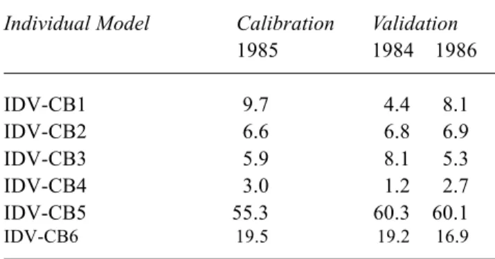
(1996). Tables 3 and 4 list the percentage of the time that each model produced the best performance on both the calibration and the validation datasets. IDV-SK1 was the best overall model at the last time step for Skelton whereas IDV-CB5 forecasts were optimal at Cefn Brwyn. For both catchments, persistence was selected on almost one in five occasions as the best previous modelling solution. This demonstrates that even the simplest method of prediction can be useful at certain times and for particular situations.

IDV-CB4 gives the best performance for the smallest amount of time, which is not at all surprising, since this model is a quasi-physical simulation tool implemented without the benefit of real-time updating.

Neural network methodologies

The next two data fusion strategies were two neural network

Table 1. Individual models

Code Model Further particulars

IDV-SK1 Hybrid neural network model See and Openshaw (1999)

IDV-SK2 Fuzzy logic model See and Openshaw (1999)

IDV-SK3 ARMA model See and Openshaw (1999)

IDV-SK4 Persistence

IDV-CB1 Neural network model (standard approach) Abrahart et al. (1999)

IDV-CB2 Neural network model developed using weight-based pruning Abrahart et al. (1999) IDV-CB3 Neural network model developed using node-based pruning Abrahart et al. (1999)

IDV-CB4 TOPMODEL Quinn and Beven (1993)

IDV-CB5 ARMA model Abrahart and See (2000)

IDV-CB6

Persistence

Table 2. Data fusion strategies Code Method

DF1 Simple calculation of an arithmetic mean for each set of forecasts. DF2 Use single best performing individual model from previous time step. DF3 Neural network amalgamation of individual forecasts based on original data. DF4 Neural network amalgamation of individual forecasts based on differenced data. DF5 Fuzzy logic combination of individual forecasts based on current record and

differences in observed record over the last six hours.

DF6 Fuzzy logic combination of individual forecasts based on current record and prediction error for single modelling solutions at last time step.

Table 3. % of time that a given model is the best performer

at Skelton

Individual Model Calibration Validation

IDV-SK1 36.2 33.6

IDV-SK2 23.5 26.4

IDV-SK3 21.1 22.2

IDV-SK4 19.2 17.8

Table 4. % of time that a given model is the best performer at Cefn Brwyn

Individual Model Calibration Validation

1985 1984 1986 IDV-CB1 9.7 4.4 8.1 IDV-CB2 6.6 6.8 6.9 IDV-CB3 5.9 8.1 5.3 IDV-CB4 3.0 1.2 2.7 IDV-CB5 55.3 60.3 60.1 IDV-CB6 19.5 19.2 16.9

solutions — constructed and computed using the method described in See and Abrahart (2001). In these experiments the individual model forecasts at the two river sites were amalgamated using feed-forward neural networks trained with the backpropagation algorithm. Two alternative implementations were undertaken, which differed in terms of their input and output data. Method three [DF3] used the absolute values of each original forecast as modelling inputs to each neural network data fusion operation. The network was then trained to forecast future river conditions on either a six-hour or one-hour ahead basis. Method four [DF4] used differenced data and a context descriptor: the absolute value of each original forecast at the forecast time step minus the observed record at the current time step, together with observed record at the current time step, provided modelling inputs to each neural network data fusion operation. The network was then trained to forecast the difference in future river conditions on either a six-hour or one-hour ahead basis. For Skelton, located on the River Ouse, the fusion input data were first split into two sets; Set 1 (Jan 1989 to Jun 1991) (60%) and Set 2 (Jul 1991 to Dec 1992) (40%). Set 1 was used to build the two fusion solutions. Set 2 was held in reserve and used to provide unseen patterns for model validation purposes. This pattern of division corresponds to the traditional proportions used in split-sample cross-validation methodologies. For Cefn Brwyn, located on the Upper River Wye, both fusion operations were calibrated using data for 1985 (April–December). Data for 1984 and 1986 (April–December) were held in reserve to provide unseen patterns for model validation purposes. This provided a stringent test since 1984 had a summer drought; 1985 contained a good spread of events; whilst 1986 showed greater divergence and experienced the biggest floods. Each neural solution was developed on a one-hidden-layer feed-forward architecture that had full connection between adjacent layers. The logistic transfer function was used in all hidden nodes and output nodes. To address problems associated with upper–limit and lower–limit saturation, both input and output data were standardised to an intermediate range (0.1 to 0.9). Network calibration was performed using the backpropagation of error algorithm — implemented with decreasing coefficients of learning and momentum. The neural networks were trained for 20 000 epochs, with trained solutions being saved at 500 epoch intervals, such that for each scenario the best performing network could then be determined from a quasi-continuous assessment of validation errors.

Soft computing methodologies

The last two data fusion strategies were two fuzzy modelling

solutions — constructed and computed using the methods described in See and Openshaw (2000). Each approach is based on a set of simple IF-THEN rules that are used to determine which combination of models should be chosen to make the next forecast based on current conditions and past model performance. For Skelton, the split between calibration and validation data was identical to that used in the two neural network data fusion operations. For Cefn Brwyn, both fusion operations were calibrated using annual data for 1985, with annual data for 1984 and 1986 being held in reserve to provide unseen patterns, for model validation purposes. It should be noted that this data fusion operation was performed on full annual data sets — albeit that the computational decision on which model to select during the first three months was restricted to input solutions that were available for the full twelve-month period. For assessment and comparison against the other modelling outputs, the numerical results from this operation are nevertheless reported in terms of the shorter nine-month period (April-December).

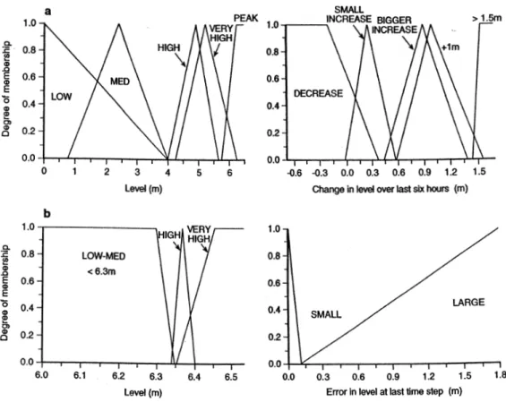
Method five [DF5] adopted a soft approach in which more than one individual modelling solution could be recommended, at each given moment, and to varying degrees. The resulting forecast at the current time step was thus a weighted average of one or more single model recommendations. DF5 used the current level (discharge) and the change in level (discharge) over the last six hours as inputs to select an appropriate model(s) and weighting(s) based on a set of fuzzy membership functions (Figs. 2a and 3a) and fuzzy logic rules (Tables 5 and 6), which had been determined and optimised using a genetic algorithm, following the method described in See and Openshaw (1999). In brief, the rule matrix, together with the parameters that defined each membership function, were first coded into digital representations and then assembled together such that: (i) each individual item comprised one single part of a string; and (ii) the error in the output forecast could be minimised. This method offers a distinct advantage over the crisp probabilistic approach since it is not forced to pick a single best individual solution.

DF5 rules for Skelton are listed in Table 5. DF5 recommends IDV-SK1 most of the time, but in particular on the rising limb of the hydrograph at LOW to HIGH levels, where LOW to HIGH are the fuzzy sets shown in Fig. 2. IDV-SK1 is also recommended on the falling limb some of the time. IDV-SK2 is recommended on the rising limb of the hydrograph at HIGH and VERY HIGH levels but not under other circumstances, which suggests that it was able to characterise this portion of the hydrograph better than the other models. IDV-SK4 is recommended at the peaks, when there is not much change, or where the water level is

Fig. 2. Fuzzy input sets for Skelton on the River Ouse: (a) DF5 and (b) DF6

exhibiting a slight rise. IDV-SK3 is recommended on the falling limb of the hydrograph and where there is a steep rise in the water level over the six-hour period. DF5 rules for Cefn Brwyn are listed in Table 6. The eleven rules identified with shaded boxes in the lower left corner did not fire during the original optimisation process, which was based on data for 1985, nor with data for 1984, but all rules fired with data for 1986. This pattern reflects the hydrological differences between each annual data set. The other fourteen rules exhibit more widespread application. IDV-CB4 is recommended on the falling limb when flow is HIGH, and during periods of LOW to MED, when the change in flow is >0.005 m2_{/h. IDV-CB1 and IDV-CB2 are}

recommended at other times. IDV-CB5 is recommended during periods of LOW and SMALL DECREASE. Neither IDV-CB6 nor IDV-CB3 is recommended in the set of fourteen rules that fired during the optimisation process.

Method six [DF6] is a fuzzification or generalisation of the crisp probabilistic approach based on the membership functions provided in Figs. 2(b) and 3(b). This method used the current level (discharge) and the forecast error at the last time step, between the observed record and each single model output, to make its recommendations. The use of current level (discharge) data allows for the selection of specific models, which are best suited to a given set of

conditions, with the potential to produce a more sensitive forecasting tool. DF6 was also optimised with a genetic algorithm. The rules reflect: (i) a crisp probabilistic approach in those situations where it was clear that one model was superior to the others and (ii) a fuzzy probabilistic approach when several models were in contention for best performer. DF6, in the latter situation, can recommend a combination of models at the current time step, which results in a weighted average based on the best solution(s) obtained at the previous time step. In this manner, the arbitrary boundary associated with choosing only the best model is fuzzified.

DF6 rules were in both cases identical, albeit that two extra rules were needed at each step, when working with six as opposed to four input data streams. DF6 rules for Skelton were listed in See and Openshaw (2000); DF6 rules for Cefn Brwyn are listed in Table 7. The first fuzzy set, i.e. LOW-MED, spans the greater part of the hydrographic domain so the first four rules will fire most of the time. It is at higher levels of discharge that the remaining rules will fire, when in most cases the error will also be LARGE. Moreover, the steep slopes characterise the rapid transition between the sets HIGH and VERY HIGH, which means that the weights applied to each of the individual model forecasts can exhibit substantial variation for small differences in error. Thus, in consequence, the fusion

Table 6. DF5 rules for Cefn Brwyn [shaded rules did not fire during calibration] Change in discharge over last six hours

DEC SM-DEC SM-INC +0.003m > 0.005 m

LOW IDV-CB1 IDV-CB5 IDV-CB1 IDV-CB1 IDV-CB4

Current MED IDV-CB4 IDV-CB2 IDV-CB2 IDV-CB1 IDV-CB4

Discharge HIGH IDV-CB4 IDV-CB2 IDV-CB5 IDV-CB1 IDV-CB4

VERY HIGH IDV-CB1 IDV-CB3 IDV-CB1 IDV-CB1 IDV-CB2

PEAK IDV-CB1 - IDV-CB1 IDV-CB4 IDV-CB2

DEC = decreasing : SM-DEC = small decrease : SM-INC = small increase

Table 5. DF5 rules for Skelton

Change in level over last six hours

DEC SM-INC BIG-INC +1m > 1.5m

LOW IDV-SK3 IDV-SK1 - IDV-SK1 IDV-SK1

Current MED IDV-SK1 IDV-SK1 IDV-SK1 IDV-SK1 IDV-SK3

Level HIGH IDV-SK1 IDV-SK1 IDV-SK1 IDV-SK2

-VERY HIGH IDV-SK3 IDV-SK1 IDV-SK2 IDV-SK2

-PEAK IDV-SK1 IDV-SK4 IDV-SK4 -

modelling output is capable of sensitive and effective responses.

Empirical results

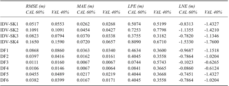
It is important to consider a number of statistical evaluators since there is no single definitive measure that can determine the success of each forecast (Houghton-Carr, 1999; Legates and McCabe, 1999; Hall, 2001). The input and output data streams for each data fusion operation are thus compared using several numerical evaluators: two global goodness-of-fit statistics (root mean squared error (RMSE) and mean absolute error of the estimate (MAE)); and two measures that record the worst possible scenarios (largest positive error (LPE) and largest negative error (LNE)). These four metrics are listed in Tables 8 and 9. The requirement to perform a direct and meaningful numerical comparison between two different stations that used two different forms of measurement also necessitated the derivation of non-dimensional assessment statistics. Nash and Sutcliffe (1970) efficiencies are for that reason recorded in Table 10. The best scores in each table are underlined. To provide qualitative information about the temporal performance of

individual forecasts and about the relative disposition of modelling errors in each data fusion solution also required detailed inspection and visual interpretation of hydrographs. Significant features are illustrated in Figs. 4 to 7.

Discussion

The validation statistics reveal that data fusion inputs from the single modelling solutions possess different properties and qualities. The best performing individual forecasters were (i) SK1 and SK3 at Skelton and (ii) IDV-CB1 and IDV-CB6 at Cefn Brwyn (but not for all metrics). In terms of data fusion there was no outright winner that spanned both catchments. The best data fusion solution for each catchment was in all but one case better than the best single modelling input; thus the data fusion process is observed to have provided some forecasting improvements. Marked differences in global error between the calibration and validation data sets, were also to some extent equalised for Cefn Brwyn. Several of the weaker data fusion solutions were nevertheless observed to be inferior in comparison to their single modelling counterparts — which implies a loss of detail or information.

Table 7. Linguistic expression of DF6 rules for Cefn Brwyn

If the current discharge [level] is LOW-MED And

the current error of IDV-CB1 is SMALL then use IDV-CB1 the current error of IDV-CB2 is SMALL then use IDV-CB2 the current error of IDV-CB3 is SMALL then use IDV-CB3 the current error of IDV-CB4 is SMALL then use IDV-CB4 the current error of IDV-CB5 is SMALL then use IDV-CB5 the current error of IDV-CB6 is SMALL then use IDV-CB6 If the current discharge [level] is HIGH And

the current error of IDV-CB1 is SMALL then use IDV-CB1 the current error of IDV-CB2 is SMALL then use IDV-CB2 the current error of IDV-CB3 is SMALL then use IDV-CB3 the current error of IDV-CB4 is SMALL then use IDV-CB4 the current error of IDV-CB5 is SMALL then use IDV-CB5 the current error of IDV-CB6 is SMALL then use IDV-CB6 If the current discharge [level] is VERY HIGH And

the current error of IDV-CB1 is SMALL Or LARGE then use IDV-CB1 the current error of IDV-CB2 is SMALL Or LARGE then use IDV-CB2 the current error of IDV-CB3 is SMALL Or LARGE then use IDV-CB3 the current error of IDV-CB4 is SMALL Or LARGE then use IDV-CB4 the current error of IDV-CB5 is SMALL Or LARGE then use IDV-CB5 the current error of IDV-CB6 is SMALL Or LARGE then use IDV-CB6

Table 8. Statistical evaluation of modelling inputs and fusion solutions for Skelton

RMSE (m) MAE (m) LPE (m) LNE (m)

CAL 60% VAL 40% CAL 60% VAL 40% CAL 60% VAL 40% CAL 60% VAL 40%

IDV-SK1 0.0517 0.0553 0.0262 0.0268 0.5074 0.5199 -0.8313 -1.4327 IDV-SK2 0.1091 0.1091 0.0454 0.0427 0.7253 0.7798 -1.1355 -1.4210 IDV-SK3 0.0823 0.0794 0.0370 0.0338 0.3755 0.3182 -0.7820 -1.1346 IDV-SK4 0.1650 0.1590 0.0720 0.0657 0.8090 0.6710 -1.5330 -1.7600 DF1 0.0868 0.0860 0.0363 0.0340 0.4634 0.3600 -0.9687 -1.1518 DF2 0.0397 0.0416 0.0162 0.0161 0.4045 0.3558 -0.7864 -1.0204 DF3 0.0111 0.0160 0.0067 0.0067 0.0744 0.5743 -0.1023 -0.6265 DF4 0.0106 0.0146 0.0067 0.0064 0.0841 0.3665 -0.0860 -0.6124 DF5 0.0455 0.0489 0.0217 0.0219 0.4044 0.3668 -0.7451 -1.4327 DF6 0.0382 0.0399 0.0167 0.0171 0.4045 0.3558 -0.7864 -1.0204

Table 9. Statistical evaluation of modelling inputs and fusion solutions for Cefn Brwyn

RMSE (m3_{h ×10}–3_{) MAE (m}3_{h ×10}–3_{) LPE (m}3_{h ×10}–3_{) LNE (m}3_{h ×10}–3₎

CAL VAL VAL CAL VAL VAL CAL VAL VAL CAL VAL VAL

1985 1984 1986 1985 1984 1986 1985 1984 1986 1985 1984 1986 IDV-CB1 0.0431 0.0611 0.0582 0.0216 0.0348 0.0274 0.9270 1.7400 1.0440 -0.8170 -0.3110 -1.0010 IDV-CB2 0.0514 0.0453 0.0638 0.0238 0.0299 0.0280 1.2800 1.5090 1.1460 -1.0610 -0.2610 -1.1930 IDV-CB3 0.0548 0.0475 0.0705 0.0264 0.0327 0.0321 0.9800 0.9830 1.3830 -1.1260 -0.2830 -1.2720 IDV-CB4 0.1416 0.1518 0.1182 0.0637 0.0556 0.0470 1.7740 4.8500 2.8320 -2.7110 -0.2490 -1.8630 IDV-CB5 0.0658 0.0398 0.0706 0.0159 0.0109 0.0162 1.5650 0.6170 1.3280 -1.3840 -1.0050 -1.1610 IDV-CB6 0.0867 0.0370 0.0975 0.0233 0.0103 0.0245 1.5360 0.3890 1.1810 -1.9140 -0.9830 -1.8580 DF1 0.0513 0.0424 0.0516 0.0188 0.0216 0.0198 0.9110 1.4360 0.8990 -1.4160 -0.1330 -1.0800 DF2 0.0608 0.0462 0.0618 0.0147 0.0089 0.0153 1.5650 1.7400 1.2320 -1.1960 -0.7830 -0.9850 DF3 0.0404 0.0588 0.0551 0.0164 0.0232 0.0200 0.8390 2.4105 1.3806 -0.9208 -0.2209 -1.0038 DF4 0.0372 0.0530 0.0509 0.0146 0.0222 0.0181 0.5111 1.7113 1.6234 -0.7996 -0.3162 -0.9968 DF5 0.0390 0.0491 0.0552 0.0125 0.0164 0.0155 0.6290 1.7400 1.2830 -0.8750 -0.4160 -1.0770 DF6 0.0335 0.0233 0.0368 0.0148 0.0180 0.0163 0.3960 0.2620 1.2320 -1.1260 -0.1820 -0.9850

DF4 was the best performer at Skelton, although both DF2 and DF6 provided a better LPE. DF4 errors were also much lower than those associated with the initial inputs which equates to the construction of a value-added solution — that has better properties or different qualities to the original material. DF6 was the best performer at Cefn Brwyn, although DF2 provided a better MAE, and mixed outcomes were obtained for LPE and LNE. DF6 statistics for this catchment were similar to those associated with the original single modelling solutions — hence, fusion has in this instance produced a limited amount of numerical refinement, or input tweaking, which amounts to an alternative set of returns. DF1 (simple averaging) produced a different

outcome at the two stations. It was the poorest of the six fusion operations at Skelton — but provided reasonable results, and on two occasions provided the best statistic, for Cefn Brwyn. The residuals from each individual model in the latter case have acted to cancel each other out, at least to some degree, which produced improved results and a practical working solution. DF2 (crisp probabilistic) produced similar or identical results to DF6 (fuzzified probabilistic) at Skelton. This result suggests that the introduction of fuzziness did not add much to the conventional probabilistic approach. DF2 produced dissimilar results to DF6 at Cefn Brwyn. DF6 was in fact the best overall performer on this occasion and the opposite

0.00 0.50 1.00 1.50 2.00 2.50 3.00 3.50 4.00 4.50 5.00 Hours Level [m] Observed IDV-SK1 IDV-SK2 IDV-SK3 IDV-SK4 0.00 0.50 1.00 1.50 2.00 2.50 3.00 3.50 4.00 4.50 5.00 Hours Level [m] Observed DF1 DF2 DF3 DF4 DF5 DF6 0.00 1.00 2.00 3.00 4.00 5.00 6.00 7.00 8.00 Hours Discharge [m cubed /hr * 1000] Observed IDV-CB1 IDV-CB2 IDV-CB3 IDV-CB4 IDV-CB5 IDV-CB6 0.00 1.00 2.00 3.00 4.00 5.00 6.00 7.00 8.00 Hours Discharge [m cubed /hr * 1000] Observed DF1 DF2 DF3 DF4 DF5 DF6

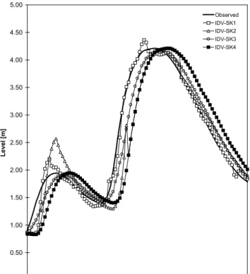
Fig. 4. Skelton: single solution forecasts for a 100 hour validation

event starting 02.00 14 Jan 1992

Fig. 5. Skelton: data fusion forecasts for a 100 hour validation event

starting 02.00 14 Jan 1992

Fig. 6. Cefn Brywn: single modelling solutions for a 35 hour

validation event starting 04.00 17 Nov 1986

Fig. 7. Cefn Brywn: data fusion forecasts for a 35 hour validation

argument can thus be applied to this smaller and flashier catchment. DF3 and DF4 (neural networks) provided similar results on both occasions — which suggests that there is little to be gained from the use of differenced data on either catchment. DF4 was the best solution at Skelton; DF4 did better than DF3 at Cefn Brwyn, albeit that neither solution was on this occasion that good, and DF3 in fact provided the worst recorded LPE. Table 10 statistics confirm that neural network fusion provided the best results at Skelton (DF3 and DF4 possess identical near-perfect scores at four decimal places) and that the best solution for Cefn Brwyn is DF6. In terms of hydrological modelling efficiencies -the best data fusion solution for Skelton is also observed to be a little bit better than the best data fusion solution for Cefn Brwyn.

Detailed inspection of hydrograph plots (i) facilitated a graphical interpretation on the range and nature of forecasting error related to single modelling and data fusion solutions and (ii) provided visual confirmation of the statistical results. Figures 4 and 5 contain exemplar hydrographs constructed from the validation data set for Skelton. IDV-SK1 (hybrid neural network forecaster) is seen to be the best single modelling solution in Fig. 4; the other single modelling solutions do less well on peaks and troughs and exhibit substantial problems throughout in the manner of a lagged response or lateral shift in output. The worst forecasts in this particular solution are the peaks — that are

Table 10. Nash and Sutcliffe Index (E) for Skelton and Cefn Brwyn Skelton Cefn Brwyn

CAL 60% VAL 40% CAL (1985) VAL (1984) VAL (1986)

INPUT IDV-SK1 0.9972 0.9947 - - -DATA IDV-SK2 0.9874 0.9793 - - -STREAM IDV-SK3 0.9929 0.9890 - - -IDV-SK4 0.9713 0.9560 - - -IDV-CB1 - - 0.9855 0.9257 0.9854 IDV-CB2 - - 0.9794 0.9592 0.9825 IDV-CB3 - - 0.9766 0.9551 0.9786 IDV-CB4 - - 0.8439 0.5412 0.9396 IDV-CB5 - - 0.9664 0.9684 0.9785 IDV-CB6 - - 0.9415 0.9728 0.9590 OUTPUT DF1 0.9921 0.9871 0.9795 0.9642 0.9885 DATA DF2 0.9983 0.9970 0.9712 0.9575 0.9835 STREAM DF3 0.9999 0.9996 0.9873 0.9310 0.9869 DF4 0.9999 0.9996 0.9892 0.9441 0.9888 DF5 0.9978 0.9958 0.9882 0.9519 0.9868 DF6 0.9985 0.9972 0.9912 0.9892 0.9942

overpredicted – this being a common problem for neural network solutions that contain no negative drivers and thus struggle to mimic the cessation of rainfall. IDV-SK4 (persistence) has the poorest match but even this solution affords a degree of correctness in terms of numerical maxima and minima and at the crossover between rising and falling limbs.

Figure 5 shows that all data fusion algorithms produced improvements. DF3 and DF4 (original data and differenced data neural network fusions) are the two best data fusion algorithms, with almost identical hydrographs, such that it is difficult to distinguish between them. Troublesome peak flow forecasts are still evident but the problem on both events is much diminished and the temporal lag has to a large extent been rectified. DF5 and DF6 provide a generalised solution that follows the general trend of the input data; peak flow prediction is better but the time lag, although diminished, is still evident throughout the range of low to moderate forecasts on each rising limb. There were strong similarities between the forecasting outputs for IDV-SK1 [hybrid neural network forecaster] and DF2, DF5 and DF6. This pattern of replication is understandable, given that IDV-SK1 was the best single modelling solution, and that fusion selection mechanisms are designed to acquire a marked preference for the most efficacious tool. DF1 (simple average) is comparable to IDV-SK3 (autoregressive moving average) and has the poorest match. This solution imitated

the general trend and produced reasonable estimates at the highest levels of prediction — but it could not correct for lagged predictions. It was also correct at the crossover between rising and falling limbs.

Figures 6 and 7 contain exemplar hydrographs constructed from the second of the two validation data sets for Cefn Brwyn. The different single modelling solutions offer a range of options, with errors that span both sides of the observed data set, and are seen to possess different qualities that offer different benefits on different occasions. It is thus difficult, if not impossible, to single out a clear-cut winner. The main problems associated with the initial predictions can nevertheless be summarised as late forecasting on rising limbs, over and underprediction on falling limbs, together with both over and underprediction of peaks and troughs. No marked irregularities or common deficiencies such as a lagged response, or universal bias, could be observed. IDV-CB6 (persistence) has the poorest match but even this solution affords a degree of correctness in terms of numerical maxima and minima and at the crossover between rising and falling limbs.

Figure 7 shows that all data fusion algorithms generated improvements. Moreover, with the exception of both peaks, the solutions exhibit a common movement towards the construction of a centralised result. DF6 (fuzzification of the crisp probabilistic approach) generated a close approximation to the observed data set; it provides an excellent fit to both major and minor flood events, and matches all other aspects of the hydrograph in a better manner than the other five data fusion strategies. DF6 demonstrated particular modelling power on the highest peak, where it provided a comprehensive forecast that was much nearer to the observed data than each single modelling solution and all other fusion mechanisms. Some outputs appeared to match the original forecasts — whereas others did not — the latter being indicative of effectual weighted behaviour. DF1, DF3, DF4 and DF5 all underpredict the most significant peak, whilst DF2 overpredicts it. DF6 also provided a similar minor underprediction on the smaller earlier peak, where it performed better, albeit closer, to the other data fusion operations. DF1 (simple average) provided a reasonable solution but was often late and struggled in difficult situations in which most models misbehaved — whilst DF2 first overpredicted the biggest peak and then provided constant underprediction of its falling limb. DF3, DF4 and DF5 provided similar solutions – such tools overpredicted the smaller peak, then underpredicted the bigger peak, which all points to neural network generalisation dilemmas and a universal failure to provide effective extrapolation on this complex data set. The lack of a best single modelling solution — on this occasion — is

thus represented in the various dissimilarities shown between DF2, DF5 and DF6. The decision making process has been forced to span a number of multiple objectives, in competition with one another, to resolve difficult problematic regions of the hydrographic record where no clear winners or fast and simple solutions exist.

The difference between these two alternative outcomes is instructive in terms of automation and incorporated wisdom. The two black-box neural network data fusion solutions were the best performers on a stable catchment that needed a simpler hydrological fix. Inputs could be merged to provide a universal approximation, in a process that doubtless benefitted from the incorporation of an available and near-perfect single modelling solution, which could impart the bulk of the forecasting information. The fuzzified crisp probabilistic approach in comparison produced slight improvements for a stable catchment based on a set of individual solutions that were both advanced and accurate. However, given more challenging hydrological problems, in terms of a flashier catchment and differing validation data sets — the neural network fusion process was less effective. Forecasting enhancements were applied to a range of medium-scale and large-scale flood events; such items were not well modelled in the original solutions. Forecasting also included extrapolation to drought conditions (1984) and to flood events larger than those found in the calibration data (1986). The weighted neural approximation was, under such circumstances, handicapped to a solution that, although non-linear, was too generalised. The situation demanded a data fusion tool that was at the same time both more powerful and more flexible in permitted responses and reactions. DF6, was in consequence, better suited to the calculation of flashier behaviour. However, it is also possible that this outcome might be related in part to the original selection of single modelling solutions, for instance with the inclusion of a simulation model that can often provide better functional approximations at the extremities of prediction.

Conclusions

The application of six multi-model data fusion methodologies for hydrological modelling, using different sites and different forecasting horizons, has been compared. Fusion improved levels of output performance and each location demonstrated various potential options and advantages in which data fusion could be used to construct superior levels of hydrological forecast. Fusion operations were better in overall terms than their individual modelling counterparts and two clear winners emerged. Indeed, the six different mechanisms on test revealed unequal aptitudes for fixing different categories of problematic catchment

behaviour; in such cases, the best method(s) were determined to be a good deal better than their closest rival(s). Neural network fusion of differenced data provided the best solution for a stable regime (with neural network fusion of original data being somewhat similar) — whereas a fuzzified probabilistic mechanism produced superior outputs in a more volatile environment.

Data fusion is seen to offer a range of fast and inexpensive methodologies. Such processes can be used to develop better hydrological forecasts, in which tried and trusted models and methods can be amalgamated and enhanced in a straightforward manner. More complex rule-based tools based on transparent science and accepted wisdom are not in all cases better. Certain fundamental problems can be addressed in a simple manner using neural networks; this suggests that more exploration and testing should be done on such topics and on other issues related to broader and smarter methods of automated generalisation. Further research will also consider alternative methods of data fusion and cover a wider range of similar or dissimilar gauging stations and catchments. There is also a pressing need to establish or delimit the role and potential of such tools and methods with regard to real time operational forecasting, or for other related purposes, which require continuous modelling solutions.

References

Abrahart, R.J. and See, L., 1999. Fusing multi-model hydrological data. Proc. Int. Joint Conf. Neural Networks, Washington, USA. [CD-ROM].

Abrahart, R.J. and See, L., 2000. Comparing neural network and autoregressive moving average techniques for the provision of continuous river flow forecasts in two contrasting catchments,

Hydrolog. Process., 14, 2157–2172.

Abrahart, R.J., See, L. and Kneale, P., 1999. Using pruning algorithms and genetic algorithms to optimise network architectures and forecasting inputs in a neural network rainfall-runoff model. J. Hydroinformatics, 1, 103–114.

Abidi, M.A. and Gonzalez, R.C., 1992. Data Fusion in Robotics

and Machine Intelligence. Academic Press, London.

Babovic, V., Canizares, R., Jensen, H.R. and Klinting, A., 2001. Neural Networks as routine for error updating of numerical models. J. Hydraul. Eng., 127, 181–193.

Brooks, R.R. and Iyengar, S.S., 1998. Multi-Sensor Fusion:

Fundamentals and Applications with Software. Prentice Hall,

Upper Saddle River, NJ.

Clemen, R.T., 1989. Combining forecasts: a review and annotated bibliography. Int. J. Forecasting, 5, 559–583.

Crowley, J.L. and Demazeau, Y., 1993. Principles and techniques for sensor data fusion. Signal Process., 32, 5–27.

Dasarathy, B.V., 1996. Fusion strategies for enhancing decision reliability in multisensor environments. Opt. Eng., 35, 603–616. Dasarathy, B.V., 1998. Decision fusion benefits assessment in a

three-sensor suite framework. Opt. Eng., 37, 354–369.

Dasarathy, B.V., 1999. Information fusion benefits delineation under off-nominal scenarios. Proc. SPIE Conf. Sensor Fusion:

Architectures, Algorithms, and Applications III, Orlando, Florida, USA. Vol. 3719. 2–13.

Dasarathy, B.V., 2000. More the merrier or is it? – Sensor suite augmentation benefits assessment. Proc. Third Int. Conf.

Information Fusion, Paris, France. Vol. 2. Paper No: WeC3-3.

Dasarathy, B.V., 2001. Information Fusion – what, where, why, when, and how? Information Fusion, 2, 75–76

Dasarathy, B.V. and Townsend, S.D., 1999. FUSE – Fusion utility sequence estimator, Proc. Second Int. Conf. Information Fusion,

Sunnyvale, California, USA. 77–84.

Hall, D.L., 1992. Mathematical Techniques in Multisensor Data

Fusion. Artech House, Boston, USA.

Hall, M., 2001. How well does your model fit the data?, J.

Hydroinformatics, 3, 49–55.

Hall, D.L. and Llinas, J., 1997. An introduction to multisensor fusion. Proc. IEEE: Special Issue on Data Fusion, 85, 6–23. Houghton-Carr, H.A., 1999. Assessment criteria for simple

conceptual daily rainfall-runoff models. Hydrolog.Sci. J., 44, 237–261.

Hu, T.S., Lam, K.C. and Ng, S.T., 2001. River flow time series prediction with a range-dependent neural network. Hydrolog.

Sci. J., 46, 729–745.

Joshi, R. and Sanderson, A.C., 1999. Multisensor Fusion: A

Minimal Representation Framework. World Scientific, London.

Knapp, B.J., 1970. Patterns of water movement on a steep upland

hillside, Plynlimon, Central Wales, Unpublished Ph.D. Thesis,

Department of Geography, University of Reading, Reading, UK. Kokar, M. and Kim, K., 1993. Review of multisensor data fusion architectures and techniques, Proc. IEEE Int. Symp. Intelligent

Control, Chicago, Illinois, USA.

Jarvie, H.P., Neal, C. and Robson, A.J., 1997. The geography of the Humber catchment. Sci. Total Environ., 194/195, 87–99. Law, M., Wass, P. and Grimshaw, D., 1997. The hydrology of the

Humber catchment. Sci. Total Environ., 194/195, 119–128. Legates, D.R. and McCabe, G.J., 1999. Evaluating the use the

“goodness-of-fit” measure in hydrologic and hydroclimatic model validation. Water Resour. Res., 35, 233–241.

Luo, R.C. and Kay, M.G., 1989. Multisensor integration and fusion in intelligent systems. IEEE Trans. Neural Networks, 19, 901– 931.

McKenna, S.A. and Poeter, E.P., 1995. Field example of data fusion in site characterization. Water Resour. Res., 31., 3229–3240. Nash, J.E. and Sutcliffe, J.V., 1970. River flow forecasting through

conceptual models, Part 1: a discussion of principles. J. Hydrol.,

10, 282–290.

Newson, M.D., 1976. The physiography, deposits and vegetation

of the Plynlimon catchments. Institute of Hydrology,

Wallingford, Oxon. Report No. 30.

Quinn, P.F. and Beven, K.J., 1993. Spatial and temporal predictions of soil moisture dynamics, runoff, variable source areas and evapotranspiration for Plynlimon, Mid-Wales. Hydrolog.

Process., 7, 425–448.

See, L. and Abrahart, R.J., 2001. Multi-model data fusion for hydrological forecasting. Comput. Geosci., 27, 987–994. See, L. and Openshaw, S., 1999. Applying soft computing

approaches to river level forecasting. Hydrolog. Sci. J., 44, 763– 778.

See, L. and Openshaw, S., 2000. A hybrid multi-model approach to river level forecasting, Hydrolog. Sci. J., 45, 523–536. Serban, P. and Askew, A.J., 1991. Hydrological forecasting and

updating procedures. IAHS Publication no. 201, 357–369. Shamseldin, A.Y. and O’Connor, K.M., 2001. A non-linear neural

network technique for updating of river flow forecasts, Hydrol.

Shamseldin, A.Y., O’Connor, K.M. and Liang, G.C., 1997. Methods for combining the outputs of different rainfall-runoff models. J. Hydrol., 197, 203–229.

Sharkey, A.J.C., 1999. Combining Artificial Neural Networks:

Ensemble and Modular Multi-Net Systems. Springer, London.

Singh, V.P., 1995. Computer Models in Watershed Hydrology. Water Resources Publications, Fort Collins, USA.

Srinivas, V.V. and Srinivasan, K., 2000. Post-blackening approach for modelling dependent annual streamflows. J. Hydrol., 230, 86–126.

Srinivas, V.V. and Srinivasan, K., 2001. Post-blackening approach for modelling periodic streamflows. J. Hydrol., 241, 221–269. Ulug, M.E. and McCullough, C.L., 2000. Quantitative metric for comparison of night vision fusion algorithms. Proc. SPIE Conf.

Sensor Fusion: Architectures, Algorithms, and Applications IV, Orlando, Florida, USA. Vol. 4051. 89–98.

Van der Voort, M., Dougherty, M.S. and Watson S.M., 1996. Combining Kohonen maps with ARIMA time series models to forecast traffic flow. Transport. Res. C, 4, 307–318.

Xiong, L., Shamseldin, A.Y. and O’Connor, K.M., 2001. A non-linear combination of the forecasts of rainfall-runoff models by the first-order Takagi-Sugeno fuzzy system, J. Hydrol., 245, 196–217.

Xydeas, C.S. and Petrovic, V.S., 2000. Objective pixel-level image fusion performance measure, Proc. SPIE Conf. Sensor Fusion:

Architectures, Algorithms, and Applications IV, Orlando, Florida, USA. Vol. 4051. 80–88.

Zhang, B. and Govindaraju, R.S., 2000. Modular neural networks for watershed runoff. Chapter 4 in: Artificial Neural Networks

in Hydrology, R.S. Govindaraju and R. Rao. (Eds.). Kluwer,