HAL Id: hal-02105124
https://hal.archives-ouvertes.fr/hal-02105124
Submitted on 20 Apr 2019
HAL is a multi-disciplinary open access
archive for the deposit and dissemination of
sci-entific research documents, whether they are
pub-lished or not. The documents may come from
teaching and research institutions in France or
abroad, or from public or private research centers.
L’archive ouverte pluridisciplinaire HAL, est
destinée au dépôt et à la diffusion de documents
scientifiques de niveau recherche, publiés ou non,
émanant des établissements d’enseignement et de
recherche français ou étrangers, des laboratoires
publics ou privés.
Asteroseismic and orbital analysis of the triple star
system HD 188753 observed by Kepler
F. Marcadon, T. Appourchaux, J. Marques
To cite this version:
F. Marcadon, T. Appourchaux, J. Marques. Asteroseismic and orbital analysis of the triple star
system HD 188753 observed by Kepler. Astronomy and Astrophysics - A&A, EDP Sciences, 2018,
617, pp.A2. �10.1051/0004-6361/201731628�. �hal-02105124�
Astronomy
&
Astrophysics
https://doi.org/10.1051/0004-6361/201731628
© ESO 2018
Asteroseismic and orbital analysis of the triple star system
HD 188753 observed by Kepler
F. Marcadon, T. Appourchaux, and J. P. Marques
Institut d’Astrophysique Spatiale, CNRS, Université Paris-Sud, Université Paris-Saclay, Bât. 121, 91405 Orsay Cedex, France e-mail: [email protected]
Received 23 July 2017 / Accepted 8 April 2018
ABSTRACT
Context. The NASA Kepler space telescope has detected solar-like oscillations in several hundreds of single stars, thereby providing a way to determine precise stellar parameters using asteroseismology.
Aims. In this work, we aim to derive the fundamental parameters of a close triple star system, HD 188753, for which asteroseismic and astrometric observations allow independent measurements of stellar masses.
Methods. We used six months of Kepler photometry available for HD 188753 to detect the oscillation envelopes of the two brightest stars. For each star, we extracted the individual mode frequencies by fitting the power spectrum using a maximum likelihood estima-tion approach. We then derived initial guesses of the stellar masses and ages based on two seismic parameters and on a characteristic frequency ratio, and modelled the two components independently with the stellar evolution code CESTAM. In addition, we derived the masses of the three stars by applying a Bayesian analysis to the position and radial-velocity measurements of the system.
Results. Based on stellar modelling, the mean common age of the system is 10.8 ± 0.2 Gyr and the masses of the two seismic com-ponents are MA= 0.99 ± 0.01 M and MBa= 0.86 ± 0.01 M . From the mass ratio of the close pair, MBb/MBa= 0.767 ± 0.006, the
mass of the faintest star is MBb= 0.66 ± 0.01 M and the total seismic mass of the system is then Msyst= 2.51 ± 0.02 M . This value
agrees perfectly with the total mass derived from our orbital analysis, Msyst= 2.51+0.20−0.18M , and leads to the best current estimate of
the parallax for the system, π= 21.9 ± 0.2 mas. In addition, the minimal relative inclination between the inner and outer orbits is 10.9◦
± 1.5◦
, implying that the system does not have a coplanar configuration.
Key words. asteroseismology – binaries: general – stars: evolution – stars: solar-type – astrometry
1. Introduction
Stellar physics has experienced a revolution in recent years with the success of the CoRoT (Baglin et al. 2006) and Kepler space missions (Gilliland et al. 2010a). Thanks to the high-precision photometric data collected by CoRoT and Kepler, asteroseismol-ogy has matured into a powerful tool for the characterisation of stars.
The Kepler space telescope yielded unprecedented data allowing the detection of solar-like oscillations in more than 500 stars (Chaplin et al. 2011) and the extraction of mode fre-quencies for a large number of targets (Appourchaux et al. 2012b; Davies et al. 2016; Lund et al. 2017). From the available sets of mode frequencies, several authors performed detailed mod-elling to infer the mass, radius, and age of stars (Metcalfe et al. 2014;Silva Aguirre et al. 2015;Creevey et al. 2017). In addition, using scaling relations, the measurement of the seismic parame-ters∆ν and νmaxprovides a model-free estimate of stellar mass
and radius (Chaplin et al. 2011, 2014). A direct measurement of stellar mass and radius can also be obtained using the large frequency separation,∆ν, angular diameter from interferometric observations, and parallax (see e.g., Huber et al. 2012; White et al. 2013). The determination of accurate stellar parameters is crucial for studying the populations of stars in our Galaxy (Chaplin et al. 2011; Miglio et al. 2013). Therefore, a proper calibration of the evolutionary models and scaling relations is required in order to derive the stellar mass, radius, and age with a high-level of accuracy. In this context, binary stars provide a
unique opportunity to check the consistency of the derived stellar quantities.
Most stars are members of binary or multiple stellar systems. Among all the targets observed by Kepler, there should be many systems showing solar-like oscillations in both components, that is, seismic binaries. However, using population synthesis mod-els, Miglio et al. (2014) predicted that only a small number of seismic binaries are expected to be detectable in the Kepler database. Indeed, the detection of the fainter star requires a mag-nitude difference between both components typically smaller than approximately one. Until now, only four systems identi-fied as seismic binaries using Kepler photometry have been reported in the literature: 16 Cyg A and B (KIC 12069424 and KIC 12069449;Metcalfe et al. 2012,2015;Davies et al. 2015), HD 176071 (KIC 9139151 and KIC 9139163; Appourchaux et al. 2012b; Metcalfe et al. 2014), HD 177412 (KIC 7510397; Appourchaux et al. 2015), and HD 176465 (KIC 10124866; White et al. 2017).
The theory of binary star formation excluded the gravita-tional capture mechanism as an explanation for the existence of binary systems (Tohline 2002). As a consequence, the binary star systems are created from the same dust disk during stellar forma-tion (Tohline 2002). Due to their common origin, both stars of a seismic binary are assumed to have the same age and initial chemical composition, allowing a proper calibration of stellar models. Indeed, the detailed modelling of each star results in two independent values of the stellar age, which can be com-pared a posteriori. In addition, ground-based observations of
A2, page 1 of15
a seismic binary also provide strong constraints on the stellar masses through the dynamics of the system. For example, the total mass of the system can be derived from its relative orbit using interferometric measurements. Among the four seismic binaries quoted above, only the pair HD 177412 has a sufficiently short period, namely ∼14 yr, to allow the determination of an orbital solution for the system. From the semi-major axis and the period of the relative orbit,Appourchaux et al.(2015) derived the total mass of the system using Kepler’s third law associated with the revised HIPPARCOS parallax of van Leeuwen(2007). However, the parallax of such a binary star can be affected by the orbital motion of the system (Pourbaix 2008), resulting in a potential bias on the estimated values of total mass and stellar radii.
Another approach for measuring stellar masses is to combine spectroscopic and interferometric observations of binary stars. This method has the advantage of allowing a direct determi-nation of distance and individual masses. Such an analysis has recently been performed by Pourbaix & Boffin (2016) for the well-known binary α Cen AB, which shows solar-like oscilla-tions in both components (Bouchy & Carrier 2002; Carrier & Bourban 2003). Thus far, α Cen AB is the only seismic binary for which both a direct comparison between the estimated val-ues of the stellar masses, using asteroseismology and astrometry, and an independent distance measurement are possible. Fortu-nately, another system offers the possibility of performing such an analysis using Kepler photometry and ground-based observa-tions. This corresponds to a close triple star system, HD 188753, for which we have detected solar-like oscillations in the two brightest components.
This article is organised as follows. Section2summarises the main features of HD 188753 and briefly describes the observa-tional data used in this work, including Kepler photometry and ground-based measurements. Section3presents the orbital anal-ysis of HD 188753 leading to the determination of the distance and individual masses. Section4details the seismic analysis of the two oscillating components, providing accurate mode fre-quencies and reliable proxies of the stellar masses and ages. Section 5 describes the input physics and optimisation proce-dure used for the detailed modelling of each of the two stars. Finally, the main results of this paper are presented and discussed in Sect.6, and some conclusions are drawn in Sect.7.
2. Target and observations
2.1. Time series and power spectrum
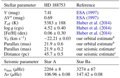
HD 188753 is a bright triple star system (V = 7.41 mag) situ-ated at a distance of 45.7 ± 0.5 pc. The main stellar parameters of the system are given in Table1. This system was observed by the Kepler space telescope in short-cadence mode (58.85 s sam-pling;Gilliland et al. 2010b) during a time period of six months, between 2012 March 29 and 2012 October 3. Standard Kepler apertures were not designed for the observation of such a bright and saturated target. A custom aperture was therefore defined and used for HD 188753, through the Kepler Guest Observer (GO) program1, to capture all of the stellar flux.
Short-cadence (SC) photometric data are available to the Kepler Asteroseismic Science Consortium (KASC; Kjeldsen et al. 2010) through the Kepler Asteroseismic Science Oper-ations Center (KASOC) database2. The SC time series for
1 https://keplergo.arc.nasa.gov/ 2 http://kasoc.phys.au.dk/
Table 1. Main stellar and seismic parameters of HD 188753.
Stellar parameter HD 188753 Reference
V(mag) 7.41 ESA(1997)
∆Va(mag) 0.69 ESA(1997)
Teff(K) 5383 ± 188 Huber et al.(2014)
log g (cgs) 4.52 ± 0.40 Huber et al.(2014) [Fe/H] (dex) 0.06 ± 0.30 Huber et al.(2014) V0(km s−1) −22.21 ± 0.03 our orbital estimateb
Parallax (mas) 21.9 ± 0.6 our orbital estimateb
Parallax (mas) 21.9 ± 0.2 our seismic estimatec
Distance (pc) 45.7 ± 0.5 our seismic estimatec Seismic parameter Star A Star Ba
νmax(µHz) 2204 ± 8 3274 ± 67
∆ν (µHz) 106.96 ± 0.08 147.42 ± 0.08
Notes. (a)Magnitude difference between the visual components.
(b)Systemic velocity and parallax derived in Sect.3.2. (c)Parallax and
corresponding distance derived in Sect.6.2.
HD 188753 (KIC 6469154) is divided into quarters of three months each, referred to as Q13 and Q14. Custom Aperture File (CAF) observations are handled differently from standard Kepler observations. A specific Kepler catalogue ID3 greater
than 100 000 000 is then assigned to each quarter. This work is based on SC data in Data Release 25 (DR25)4, which were
processed with the SOC Pipeline 9.3 (Jenkins et al. 2010). As a result, the DR25 SC light curves were corrected for a calibration error affecting the SC pixel data in DR24.
The light curves were concatenated and high-pass filtered using a triangular smoothing with a full width at half max-imum (FWHM) of one day to minimise the effects of long-period instrumental drifts. The single-sided power spectrum was produced using the Lomb-Scargle periodogram (Lomb 1976; Scargle 1982), which has been properly calibrated to comply with Parseval’s theorem (seeAppourchaux 2014). The length of data gives a frequency resolution of about 0.06 µHz. Figure1 shows the smoothed power spectrum of HD 188753 with a zoom-in on the oscillation modes of the secondary seismic com-ponent at ∼3300 µHz. The significant peak in the PSPS lies at ∆ν/2 ' 74 µHz, where ∆ν is the large frequency separa-tion; it corresponds to the signature of the near-regular spacing between individual modes of oscillation for the secondary com-ponent. Table1provides the seismic parameters of the two stars, ∆ν and νmax, as derived in Sect. 4.2. We note that previous
DR24 did not allow the detection of the secondary compo-nent in the SC light curves due to the degraded signal-to-noise ratio (S/N).
2.2. Astrometric and radial-velocity data
HD 188753 (HIP 98001, HO 581, or WDS 19550+4152) is known as a close visual binary discovered byHough(1899) and charac-terised by an orbital period of ∼25 yr (van Biesbroeck 1918). In the late 1970s, it was established that the secondary component is itself a spectroscopic binary with an orbital period of ∼154 days (Griffin 1977). HD 188753 is thus a hierarchical triple star system
3 Kepler IDs are 100 004 033 and 100 004 071 for Q13 and Q14
respectively.
Fig. 1.Power spectrum of HD 188753. Left panel: power spectrum smoothed with a 1 µHz boxcar filter showing the oscillation modes of the two seismic components around 2200 and 3300 µHz, respectively. Right panel: zoom-in on the mode power peaks of the secondary component. The inset displays the power spectrum of the power spectrum (PSPS) computed over the frequency range of the oscillations around νmax= 3274±67 µHz
(see Table1).
consisting of a close pair (B) in orbit at a distance of 11.8 AU from the primary component (A).
Position measurements of HD 188753 were first obtained by Hough (1899) with the 181/
2 inch Refractor of the
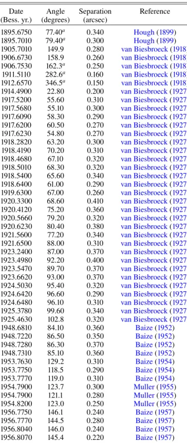
Dear-born Observatory of Northwestern University. This system was then continuously observed over the last century using differ-ent techniques and instrumdiffer-ents. Since the pioneering work of Struve (1837), more than 150 yr of micrometric measurements are now available for double stars in the literature. TableA.1 pro-vides the result of the micrometric observations for HD 188753. In addition, speckle interferometry for getting the relative posi-tion of close binaries has been in use since the 1970’s (Labeyrie et al. 1974). These observations are included in the Fourth Cat-alog of Interferometric Measurements of Binary Stars (Hartkopf et al. 2001b)5. Table A.2 summarises the high-precision data
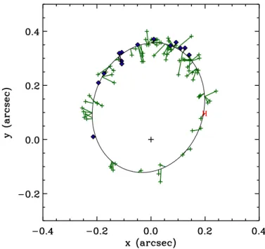
obtained for HD 188753 from 1979 to 2006. All published data of HD 188753 are displayed in Fig.2.
The first radial-velocity (RV) observations of HD 188753 were performed by Griffin (1977) from 1969 to 1975 using the photoelectric RV spectrometer of the Cambridge Observa-tories described in Griffin (1967). The author then discovered that the system contained a spectroscopic binary with an orbital period of ∼154 days. HD 188753 was later observed byKonacki (2005) with the high-resolution echelle spectrograph (HIRES; Vogt et al. 1994) at the W. M. Keck Observatory, from 2003 August to 2004 November. Konacki reported the detection of a hot Jupiter around the primary component that was chal-lenged byEggenberger et al.(2007). However, the author showed that the spectroscopic binary detected by Griffin (1977) cor-responds to the secondary component of the visual pair. The system was finally observed byEggenberger et al.(2007) with the ELODIE echelle spectrograph (Baranne et al. 1996) at the Observatoire de Haute-Provence (France) between July 2005 and August 2006. In order to derive the radial velocities of the faintest star, Mazeh et al. (2009) applied a three-dimensional (3D) correlation technique (TRIMOR) to the data obtained by Eggenberger et al.(2007). In this study, we used the RV mea-surements fromGriffin(1977),Konacki(2005), andMazeh et al. (2009).
5 http://ad.usno.navy.mil/wds/int4.html
Fig. 2. Astrometric orbit of HD 188753. Micrometric observations are indicated by green plus symbols and interferometric observations by blue diamonds. The green lines indicate the distance between the observations and the fitted orbit. A red “H” indicates the HIPPARCOS measure. East is upwards and north is to the right.
3. Orbital analysis
3.1. Method and model
In this section, we present the methodology employed to deter-mine the orbital parameters of the triple star system HD 188753. For this, we performed a combined treatment of more than a century of archival astrometry (AM) along with the RV measurements found in the literature.
Recently, Appourchaux et al. (2015) derived the orbit of the seismic binary HD 177412 (HIP 93511) by applying a Bayesian analysis to the astrometric measurements of the sys-tem. We adapted this Bayesian approach in order to include the
radial-velocity measurements for HD 188753. We defined the global likelihood of the data given the orbital parameters as:
L= LAMLRV, (1)
where LAMand LRVare the likelihoods of the AM and RV data
respectively, computed from:
ln LAM= − 1 2 NAM X i=1 xmod i − x obs i σx,i 2 + ymod i −y obs i σy,i 2 , (2) ln LRV= − 1 2 NRV X i=1 Vmod i − V obs i σV,i 2 . (3)
NAMand NRVdenote the number of available AM and RV
obser-vations, respectively, and σ refers to the associated uncertainties. The terms x and y correspond to the coordinates of the orbit on the plane of the sky and denote the declination and right ascen-sion differences, respectively. The term V stands for the radial velocities. The exponents “mod” and “obs” refer to the mod-elled and observed constraints used during the fitting procedure. Here, the observed positions xobsand yobsare computed from the measured quantities (ρ, θ) by means of the simple relations x= ρ cos θ and y = ρ sin θ, where ρ is the relative separation and θ is the position angle for both components. AppendixAprovides the values of ρ and θ derived from the micrometric and interfer-ometric measurements of HD 188753. In addition, the RV obser-vations Vobsused in this work can be found in Griffin (1977),
Konacki(2005), andMazeh et al.(2009). The theoretical values in Eqs. (2) and (3), namely xmod, ymod, and Vmod, are calculated
from the orbital parameters of the system following the observ-able model described in AppendixB. For the derivation of these orbital parameters, that is, Porb = (P, T, V0, KA, KB, e, ω, a, i, Ω),
we employed a Markov chain Monte Carlo (MCMC) method using the Metropolis-Hastings algorithm (MH;Metropolis et al. 1953;Hastings 1970) as explained in AppendixC.
An essential aspect when combining different data types is the determination of a proper relative weighting. To this end, we performed a preliminary fit of each data set either coming from astrometry or from RV measurements, and calculated the root mean square (rms) of the residuals. AppendixDprovides the residual rms derived from the RV measurements of the dif-ferent authors. In the same way, we derived the residual rms on xand y by fitting the micrometric and interferometric measure-ments independently. For micrometric measuremeasure-ments, we found σx= 25 mas and σy= 34 mas while for interferometric
measure-ments, we found σx = 6 mas and σy = 11 mas. We used these
values determined after the fitting as weights for the combined fit.
3.2. Orbit of the AB system
We applied the methodology described above in order to derive the best-fit orbital solution of the visual pair, hereafter referred to as the AB system. However, the RV measurements need to be reduced from the 154-day modulation induced by the close pair, hereafter referred to as the Bab sub-system. We then fitted this 154-day modulation as described in Sect. 3.3 (see also AppendixD) to obtain the long-period orbital motion of the AB system.
Figure2shows the best-fit solution of the astrometric orbit, plotted with all micrometric and interferometric data listed in
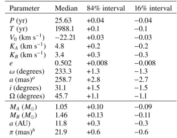
Table 2. Orbital and physical parameters of the AB system.
Parameter Median 84% interval 16% interval
P(yr) 25.63 +0.04 −0.04 T (yr) 1988.1 +0.1 −0.1 V0(km s−1) −22.21 +0.03 −0.03 KA(km s−1) 4.8 +0.2 −0.2 KB(km s−1) 3.4 +0.3 −0.3 e 0.502 +0.008 −0.008 ω (degrees) 233.3 +1.3 −1.3 a(mas)a 258.7 +2.8 −2.7 i(degrees) 31.1 +1.5 −1.5 Ω (degrees) 45.7 +1.1 −1.1 MA(M ) 1.05 +0.10 −0.09 MB(M ) 1.46 +0.13 −0.11 a(AU) 11.8 +0.3 −0.3 π (mas)b 21.9 +0.6 −0.6
Notes.(a)mas is milliarcsecond.(b)Orbital parallax derived in Sect.3.2.
AppendixA. The position of the primary component is marked by a plus symbol at the origin of the axes. O − C residuals of the orbital solution are indicated by the solid lines connecting each observation to its predicted position along the orbit. We note that this orbit is listed as grade 1 in the Sixth Catalog of Orbits of Visual Binary Stars (Hartkopf et al. 2001a)6, on a scale of 1 (“definitive”) to 5 (“indeterminate”), corresponding to a well-distributed coverage exceeding one revolution. In Fig.3, we also plotted the radial velocities of the two visual compo-nents computed from our best-fit solution. The black line denotes the RV solution of the A component, i.e. the single star, while the grey line denotes the RV solution of the Bab sub-system. For comparison, we added the RV measurements from Griffin (1977),Konacki(2005), andMazeh et al.(2009), after having removed the 154-day modulation. The final orbital parameters determined from the best-fit solution are given in Table2.
From these parameters, we can derive the mass of the two components and the semi-major axis of the visual orbit (Heintz 1978): MA= 1.036 × 10⁻⁷(K A+ KB)2KBP(1 − e2)3/2 sin3i , (4) MB= 1.036 × 10⁻⁷(KA+ KB)2KAP(1 − e2)3/2 sin3i , (5) aAU= 9.192 × 10⁻⁵(K A+ KB) P (1 − e2)1/2 sin i , (6)
where MA and MBare expressed in units of the solar mass and
aAUis expressed in astronomical units. Here, KAand KBare the
semi-amplitudes of the radial velocities for both components, in km s−1, P is the orbital period, in days, e is the eccentricity and i is the inclination of the plane of the orbit to the plane of the sky. In addition, the parallax of the system can be determined from the following ratio by combining the AM and RV results: πmas=
amas
aAU
, (7)
where πmas is expressed in milliarcseconds. Here, amas denotes
the angular semi-major axis derived from the fitting procedure
Fig. 3.Radial velocities of the two visual components. Left panel: RV measurements of the primary (blue) and secondary (red) components after having removed the 154-day modulation. Squares, circles, and diamonds denote the radial velocities fromGriffin(1977),Konacki(2005), and
Mazeh et al.(2009), respectively. Right panel: zoom-in on the RV measurements ofMazeh et al.(2009) to show the quality of the fit. The black line denotes the RV solution of the A component while the grey line denotes the RV solution of the B component.
and given in Table 2 while aAU denotes the linear semi-major
axis defined in Eq. (6). Table 2 provides the results of the above equations. In order to derive the median and the credible intervals of each physical parameter, namely MA, MB, aAU, and
πmas, we calculated Eqs. (4)–(7) using the chains of the orbital
parameters.
We found the orbital masses for the single star and the Bab sub-system to be MA = 1.05+0.10−0.09M and MB = 1.46+0.13−0.11M ,
respectively. The total mass of the triple star system is then Msyst = 2.51+0.20−0.18M . Additionally, the orbital parallax of the
system was found to be π= 21.9 ± 0.6 mas. A comparison with the literature results is presented in Sect.6.2.
3.3. Orbit of the Bab sub-system
To demonstrate the capacity of their new algorithm, TRIMOR, Mazeh et al. (2009) re-analysed the spectra of HD 188753 obtained byEggenberger et al.(2007). As a result, they derived the radial velocities of the three stars, allowing them to clas-sify the close pair as a double-lined spectroscopic binary (SB2). We then applied our Bayesian analysis to the RV measurements provided byMazeh et al.(2009) in their Table 1.
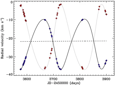
Figure4shows the best-fit solution of the radial velocities for both components of the Bab sub-system. We note that in our analysis, we included a linear drift corresponding to the long-period orbital motion of the Bab sub-system. The linear drift and the orbital parameters of the close pair, determined from our best-fit solution, are given in TableD.5. In particular, the Bab sub-system has an eccentricity of 0.175 ± 0.002 and an orbital period of 154.45 ± 0.09 days.
In the case of double-lined spectroscopic binaries, only the quantities MAsin3iand MBsin3ican be derived from Eqs. (4)
and (5). These quantities thus provide a lower limit of the stel-lar masses and a direct estimate of the mass ratio between both stars. From the orbital parameters of the close pair, presented in TableD.5, we obtained MBasin3iBab= 0.258 ± 0.004 M and
MBbsin3iBab = 0.198 ± 0.002 M . Here, iBab denotes the
incli-nation of the Bab sub-system relative to the plane of the sky. The mass ratio of the close pair is then found to be MBb/MBa=
0.767 ± 0.006, in agreement with the value of 0.768 ± 0.004
Fig. 4. RV measurements of the Ba (blue) and Bb (red) components from Mazeh et al. (2009). The dashed line denotes the long-period orbital motion of the close pair and corresponds to a linear drift towards the positive radial velocities, as can be seen in the right panel of Fig.3. The black line denotes the RV solution of the Ba component, that is, the most massive star of the close pair, while the grey line denotes the RV solution of the Bb component, the faintest companion.
provided byMazeh et al. (2009). We note that our error esti-mate of the mass ratio is somewhat larger than that ofMazeh et al. (2009). We suspect that the authors underestimate the uncertainties on their orbital parameters, used in the calcula-tion of the mass ratio, in comparison with our derived values and those of Eggenberger et al. (2007). The advantage of our Bayesian approach is that it yields credible intervals at 16% and 84%, corresponding to the frequentist 1-σ confidence intervals. In the case of HD 188753, the inclination of the close pair can be estimated from its spectroscopic mass sum MBsin3iBab =
0.456 ± 0.006 M . Indeed, the total mass of the Bab sub-system,
MB = 1.46+0.13−0.11M , is known from the orbital analysis of the
visual pair (see Sect. 3.2). The inclination of the close pair is then found to be iBab = 42.8◦± 1.5◦. In addition, we previously
determined the inclination of the AB system, listed in Table2, from our combined analysis of the visual orbit. This corresponds to a minimal relative inclination (MRI) between the two orbits of 11.7◦± 1.7◦. The implications of the MRI for such a triple star
system will be discussed in Sect.6.3.
Finally, the inclination iBab can be injected in the quantities
MBasin3iBab = 0.258 ± 0.004 M and MBbsin3iBab = 0.198 ±
0.002 M in order to derive the individual masses for both stars
of the close pair. We found the orbital masses for stars Ba and Bb to be MBa= 0.83 ± 0.07 M and MBb= 0.63+0.06−0.05M ,
respec-tively. In the following, we will compare the orbital masses determined for the three stars of the system with the results of the stellar modelling.
4. Seismic data analysis
The goal of this section is to derive accurate mode frequencies and reliable proxies of the stellar masses and ages for the two seismic components of HD 188753. These quantities will then be used for the detailed modelling of each of the two components as explained in Sect.5.2.
4.1. Mode parameter extraction
The extraction of accurate mode frequencies for the two seis-mic components of HD 188753 is an important step before the stellar modelling. In this work, we adopted a maximum likelihood estimation approach (MLE;Anderson et al. 1990) fol-lowing the procedure described inAppourchaux et al.(2012b), which has been extensively used during the nominal Kepler mis-sion to provide the mode parameters of a large number of stars (Appourchaux et al. 2012a,b,2014,2015).
We repeat here the different steps of this well-suited proce-dure for completeness:
1. We derive initial guesses of the mode frequencies for the fitting procedure by applying an automated method of detec-tion (seeVerner et al. 2011, and references therein) which is based on the values of the seismic parameters, νmaxand∆ν,
that are manually tweaked if required.
2. We fit the power spectrum as the sum of a stellar back-ground made up of a combination of a Lorentzian profile and white noise, as well as a Gaussian oscillation mode enve-lope with three parameters (the frequency of the maximum mode power, the maximum power, and the width of the mode power).
3. We fit the power spectrum with n orders using the mode profile model described inAppourchaux et al.(2015), with no rotational splitting and the stellar background fixed as determined in step 2.
4. We repeat step 3 but leave the rotational splitting and the stellar inclination angle as free parameters, and then apply a likelihood ratio test to assess the significance of the fitted splitting and inclination angle.
The steps above were used for the main mode power at 2200 µHz, and repeated for the mode power at 3300 µHz. We note that for the secondary component, we used the residual power spectrum derived from the fit of the primary. It corresponds to the ratio between the observed power spectrum and the best fitting model of the primary component, which includes a Lorentzian pro-file for the stellar background. As a result, the background was modelled with a single white noise component when fitting the mode power at 3300 µHz. The procedure for the quality assur-ance of the frequencies obtained for both stars is described in Appourchaux et al.(2012b) with a slight modification (for more
details, seeAppourchaux et al. 2015). The frequencies and their formal uncertainties, derived from the inverse of the Hessian matrix, are provided in AppendixE.
4.2. Stellar parameters from scaling relations
Using the seismic parameters given in Table1for stars A and Ba, it is possible to determine their stellar parameters without further advanced modelling. Indeed, the stellar mass and radius of the two seismic components can be estimated from the well-known scaling relations: M M = νmax νref !3 ∆ν ∆νref !−4 T eff Teff, !3/2 , (8) R R = νmax νref ! ∆ν ∆νref !−2 T eff Teff, !1/2 , (9)
where νmaxis the frequency of maximum oscillation power,∆ν
is the large frequency separation, and Teff is the effective
tem-perature of the star. Here, we adopted the reference values from Mosser et al.(2013), νref= 3104 µHz and ∆νref= 138.8 µHz, and
the solar effective temperature, Teff, = 5777 K.
For each seismic component, we derived νmax by fitting a
parabola over four (star Ba) or five (star A) monopole modes around the maximum of mode height and ∆ν by fitting the asymptotic relation for frequencies (Tassoul 1980). For star A, we obtained νmax= 2204 ± 8 µHz and ∆ν = 106.96 ± 0.08 µHz,
while for star Ba, we obtained νmax = 3274 ± 67 µHz and ∆ν =
147.42 ± 0.08 µHz. In this work, we adopted the spectroscopic values of the effective temperature fromKonacki(2005), Teff,A=
5750 ± 100 K and Teff,Ba = 5500 ± 100 K, measured
indepen-dently for stars A and Ba. Using Eqs. (8) and (9) with the above values, we then obtained MA= 1.01 ± 0.03 M and RA=
1.19 ± 0.01 R for star A, and MBa= 0.86 ± 0.06 M and RBa=
0.91 ± 0.02 R for star Ba. The effective temperature of Ba is
contaminated by that of Bb. Due to the flux ratio of about 1 to 9 as measured byMazeh et al. (2009), the temperature of Ba is likely to be 3% lower. With the effective temperature bias due to Bb, the mass and the radius of Ba would be lower by 0.04 M , 0.015 R , respectively; still commensurate with the
ran-dom errors. We also deduced the luminosity of the two stars from the Stefan–Boltzmann law, L ∝ R2T4
eff, as LA= 1.40 ± 0.12 L
and LBa = 0.69 ± 0.07 L (with a bias of −0.1 L due to the
presence of Bb).
Consequently, provided that a measurement of Teff is
avail-able, the seismic parameters νmaxand∆ν give a direct estimate of
the stellar mass and radius independent of evolutionary models. This so-called direct method has been applied to the hundreds of solar-type stars for which Kepler has detected oscillations (Chaplin et al. 2011,2014). In the case of HD 188753, the masses derived for each star from the direct method are consistent with the results of our orbital analysis. Therefore, these estimates provide an initial range of mass for stellar modelling.
4.3. Frequency separation ratios
In this work, we used the frequency separation ratios as observa-tional constraints for the model fitting, instead of the individual frequencies themselves. Indeed,Roxburgh & Vorontsov(2003) demonstrated that the frequency ratios are approximately inde-pendent of the structure of the outer layers and are determined only by the internal structure of the star. They are therefore less
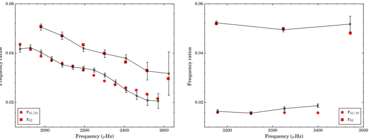
2000 2200 2400 2600 Frequency (µHz) 0.02 0.04 0.06 F re qu en cy ra ti os r01/10 r02 3200 3300 3400 3500 Frequency (µHz) 0.02 0.04 0.06 F re qu en cy ra ti os r01/10 r02
Fig. 5.Frequency separation ratios as a function of frequency for star A (left) and star Ba (right). The ratios r01/10(n) and r02(n) derived from the
reference model of each star are indicated by red circles and squares, respectively, while the observed ratios are shown as connected points with errors.
sensitive than the individual frequencies to the improper mod-elling of the near-surface layers (Roxburgh 2005; Otí Floranes et al. 2005) and are also insensitive to the line-of-sight Doppler velocity shifts (Davies et al. 2014). The use of these ratios then allows us to avoid potential biases from applying frequency corrections for near-surface effects (e.g. Kjeldsen et al. 2008; Gruberbauer et al. 2013;Ball & Gizon 2014a,b) and for Doppler shifts.
The frequency separation ratios are defined as: r02(n)= d02(n) ∆1(n) , (10) r01(n)= d01(n) ∆1(n) , r10(n)= d10(n) ∆0(n+ 1) , (11)
where d02(n) = νn,0 −νn−1,2 and ∆l(n) = νn,l−νn−1,l refer to
the small and large separations, respectively. Here, we adopted the five-point smoothed small frequency separations following Roxburgh & Vorontsov(2003):
d01(n)= 1 8(νn−1,0− 4νn−1,1+ 6νn,0− 4νn,1+ νn+1,0), (12) d10(n)= − 1 8(νn−1,1− 4νn,0+ 6νn,1− 4νn+1,0+ νn+1,1), (13)
where ν is the mode frequency, n is the radial order and l is the angular degree. In Fig.5, we plotted for both stars the ratios r01,
r10 and r02 computed from the observed frequencies. A clear
oscillatory behaviour of the observed frequency ratios can be seen for star A, in the left panel of Fig.5, indicating an acoustic glitch. Such a signature arises from the acoustic structure and has already been detected in other solar-like stars (Mazumdar et al. 2014).
Another advantage of using the frequency ratios is that the ratio r02is sensitive to the structure of the core and hence to the
age of the star (Otí Floranes et al. 2005;Lebreton & Montalbán 2009). In particular,White et al.(2011) used the ratio r02instead
of the small frequency separation to construct a modified version of the so-called C-D diagram (Christensen-Dalsgaard 1984), showing that this ratio is an effective indicator of the stellar
age. In the case of HD 188753, the mean values of the mea-sured ratios, averaged over the whole range of the observed radial orders, are hr02iA = 0.043 ± 0.001 and hr02iBa= 0.051 ± 0.001.
From these values and those of the large frequency separation listed in Table 1, we can then determine the position of the two seismic components in the modified C-D diagram obtained by White et al.(2011). Using their Fig. 8, we found an age of ∼11 Gyr for star A and of ∼8.0 Gyr for star Ba.
In addition, Creevey et al.(2017) recently derived a linear relation between the mean value of r02 and the stellar age from
the analysis of 57 stars observed by Kepler. Using their Eq. (6) with the above values of hr02i, we found the individual ages for
stars A and Ba to be 9.5 ± 0.2 Gyr and 8.0 ± 0.2 Gyr, respec-tively. We point out that our estimated errors only result from the propagation of the uncertainties on the measured ratios, since Creevey et al.(2017) do not provide uncertainties on their fitted parameters. The use of the ratio r02 as a proxy of the stellar age
therefore allows us to derive an initial range of age for stellar modelling.
5. Stellar modelling
5.1. Input physics
In order to determine precise stellar parameters for HD 188753, we performed a detailed modelling of each seismic component using the stellar evolution code CESTAM (Code d’Évolution Stellaire, avec Transport, Adaptatif et Modulaire; Morel & Lebreton 2008;Marques et al. 2013).
For our model calculations, we adopted the 2005 version of the OPAL equation of state (Rogers & Nayfonov 2002) and the OPAL opacities (Iglesias & Rogers 1996) complemented by those of Alexander & Ferguson (1994) for low tempera-tures. The opacity tables are given for the new solar mixture derived byAsplund et al.(2009), which corresponds to (Z/X) =
0.0181. The microscopic diffusion of helium and heavy ele-ments, including gravitational settling, thermal and concentra-tion diffusion, but no radiative levitaconcentra-tion, was taken into account following the prescription ofMichaud & Proffitt(1993). We used the NACRE nuclear reaction rates (Angulo et al. 1999) with the revised14N(p, γ)15O reaction rate fromFormicola et al.(2004). Convection was treated according to the mixing-length theory
(MLT; Böhm-Vitense 1958) and no overshooting was consid-ered. A standard Eddington gray atmosphere was employed for the atmospheric boundary condition.
5.2. Model optimisation
For each seismic component of HD 188753, we constructed a grid of stellar evolutionary models using CESTAM with the input physics described above. The goodness of fit was evalu-ated for all of the grid models from the merit function χ2given
by: χ2 = (x
mod− xobs)TC−1(xmod− xobs), (14)
where xobsdenotes the observational constraints considered, that
is, the frequency ratios defined in Eqs. (10) and (11), where xmoddenotes the theoretical values predicted by the model and
T denotes the transposed matrix. Here, C refers to the covariance matrix of the observational constraints, which is not diagonal due to the strong correlations between the frequency ratios. The theoretical oscillation frequencies used for the calculation of the frequency ratios were computed with the Aarhus adiabatic oscillation package (ADIPLS;Christensen-Dalsgaard 2008).
Firstly, a total of 2000 random grid points were drawn for each star from a reasonable range of the stellar parameters, these being, the age of the star, the mass M, the initial helium abundance Y0, the initial metal-to-hydrogen ratio (Z/X)0 and
the mixing-length parameter for convection αMLT. Following the
age-hr02i relation ofCreevey et al.(2017), the age of the two stars
was assumed to be in the range 5–13 Gyr. For stars A and Ba, we adopted MA ∈ [0.9, 1.2] M and MBa∈ [0.7, 1.0] M ,
respec-tively, in agreement with the results of the orbital analysis and scaling relations. We considered Y0 ∈ [YP, 0.31] where YP =
0.2477 ± 0.0001 is the primordial value from standard Big Bang nucleosynthesis (Planck Collaboration XVI 2014). The present (Z/X) ratio can be derived from the observed [Fe/H] value, provided in Table1, through the relation [Fe/H] = log(Z/X) − log(Z/X) . We then estimated the initial [Z/X]0ratio as being in
the range 0.01–0.05, which was shifted to a higher value to com-pensate for diffusion. We adopted αMLT ∈ [1.6, 2] following the
solar calibration ofTrampedach et al.(2014) that corresponds to
αMLT, = 1.76 ± 0.04.
Secondly, in order to determine the final parameters of the two stars, we employed a Levenberg–Marquardt minimisation method using the Optimal Stellar Models (OSM)7 software
developed by R. Samadi. For star A, we selected the 50 grid models with the lowest χ2 values and used them as a
start-ing point for the final optimisation. We then performed a set of local minimisations adopting the age of the star, the mass, the initial helium abundance, the initial (Z/X)0 ratio and the
mixing-length parameter as free model parameters. Again, we adopted the merit function defined in Eq. (14) associated with the frequency ratios. For star Ba, due to the limited number of observed ratios, we decided to only adjust the age, the mass, and the initial helium abundance. We then performed a first set of minimisations from the 15 grid models with the lowest χ2 values. During the minimisation process, the initial (Z/X)0ratio
and the mixing-length parameter were fixed at the value of the grid point considered. In order to explore the impact of changing these parameters, we performed a second set of minimisations for the 15 grid models previously selected adopting (Z/X)0 =
[0.015, 0.025, 0.035, 0.045] and αMLT = [1.65, 1.75, 1.85, 1.95]
7 https://pypi.python.org/pypi/osm
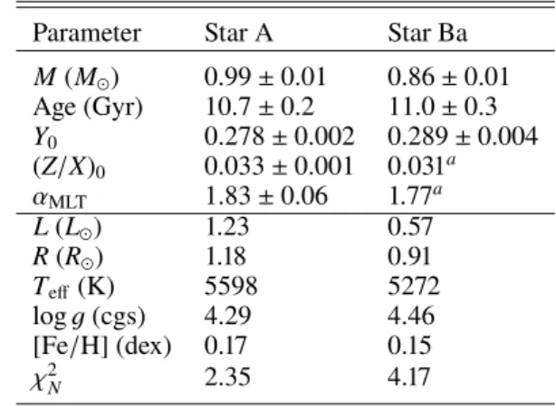
Table 3. Reference models for star A and star Ba.
Parameter Star A Star Ba
M(M ) 0.99 ± 0.01 0.86 ± 0.01 Age (Gyr) 10.7 ± 0.2 11.0 ± 0.3 Y0 0.278 ± 0.002 0.289 ± 0.004 (Z/X)0 0.033 ± 0.001 0.031a αMLT 1.83 ± 0.06 1.77a L(L ) 1.23 0.57 R(R ) 1.18 0.91 Teff(K) 5598 5272 log g (cgs) 4.29 4.46 [Fe/H] (dex) 0.17 0.15 χ2 N 2.35 4.17
Notes.(a)The reference model of star Ba was obtained for (Z/X) 0and
αMLT fixed at their grid-point values during the minimisation process
(see text).
as fixed values. In total, the number of local minimisations for star Ba was 15+ 4 × 4 × 15 = 255. We note that our reference model of star Ba, provided in Table3, was obtained for (Z/X)0
and αMLTfixed at their grid-point values.
Figure 5 shows the comparison of the observed frequency ratios (black crosses) with the corresponding values derived from the reference model of each star (red symbols). The mod-elling results for stars A and Ba are given in Table3. The error bars on the stellar parameters were derived from the inverse of the Hessian matrix. The normalised χ2values were computed as χ2
N= χ
2/N where N denotes the number of observed frequency
ratios used for the optimisation.
6. Results and discussion
6.1. Physical parameters of HD 188753
From the modelling, we found the individual ages for stars A and Ba to be 10.7 ± 0.2 Gyr and 11.0 ± 0.3 Gyr, respectively. These values are consistent within their error bars, as expected from the common origin of both stars. Combining the individual ages, the system is then about 10.8 ± 0.2 Gyr old.
In addition, the stellar masses from our reference models were found to be MA = 0.99 ± 0.01 M and MBa = 0.86 ±
0.01 M , which agree very well with the results of the orbital
analysis and scaling relations. This latter value can be injected in the mass ratio of the close pair derived in Sect.3.3, MBb/MBa=
0.767 ± 0.006, in order to determine the mass of the faintest star with much more precision than in our orbital analysis. The seismic mass of the star Bb is then found to be MBb =
0.66 ± 0.01 M . As a result, the seismic mass of the Bab
sub-system is MB= 1.52 ± 0.02 M and the total seismic mass of the
triple star system is Msyst = 2.51 ± 0.02 M . This method
pro-vides a precise but model-dependent total mass of the system, which can be compared with the results of our orbital analysis. Indeed, as explained in Sect.3.2, we obtained a direct estimate of the total mass, Msyst = 2.51+0.20−0.18M , using the astrometric
and RV observations of the system. We find excellent agree-ment between the seismic and orbital values of the total mass for HD 188753, bolstering our confidence in the results of the stellar modelling.
Our stellar models thus provide precise and accurate val-ues of the individual masses that can be used to refine the physical parameters of the system. For example, the semi-major
axis of the relative orbit is related to the total mass and to the orbital period of the system from the Kepler’s third law. In other words, the total mass of the system expressed in units of the solar mass is given by Msyst = a3AU/P2, where aAUis the
semi-major axis expressed in astronomical units and P is the orbital period expressed in years. Using the Kepler’s third law with the total seismic mass and the orbital period of the AB system, Msyst = 2.51 ± 0.02 M and P= 25.63 ± 0.04 yr, we find that
the semi-major axis of the relative orbit for the visual pair is aAU= 11.82 ± 0.03 AU. Furthermore, by applying the definition
of the centre of mass to the AB system, we can also derive the semi-major axis of the two barycentric orbits with:
aA= aAU MB MA+ MB and aB= aAU MA MA+ MB , (15)
where, obviously, aAU= aA+ aB. Adopting the seismic masses
MA = 0.99 ± 0.01 M and MB = 1.52 ± 0.02 M and the above
value of the semi-major axis aAU, we then obtain aA = 7.17 ±
0.04 AU and aB = 4.65 ± 0.03 AU. Similarly, the Kepler’s third
law and the definition of the centre of mass can be applied to the Bab sub-system using the seismic masses of the close pair. From the above values of MBa and MBb, associated with an orbital
period of 154.45 ± 0.09 days, we find that the semi-major axes for star Ba and star Bb are aBa= 0.282 ± 0.002 AU and aBb =
0.367 ± 0.002 AU, respectively. 6.2. Asteroseismic parallax
As explained in Sect.3.2, the astrometric and RV observations of the visual pair can be combined in order to derive the parallax of the system. The term “orbital parallax” has been suggested to denote a parallax determined in this way (Armstrong et al. 1992). From our combined analysis of the visual pair, we then obtained an orbital parallax of π= 21.9 ± 0.6 mas.
In the case of HD 188753, the precision on the parallax can be improved using the total seismic mass of the system deter-mined in Sect.6.1. Indeed, combining the Kepler’s third law with Eq. (7) provides a direct relation between the total mass and the parallax of the system:
Msyst = amas πmas !3 1 P2, (16)
where Msyst is expressed in units of the solar mass and πmas is
expressed in milliarcseconds. Here, amas is the angular
semi-major axis of the visual pair, in mas, and P is the orbital period, in years. Adopting the total seismic mass Msyst= 2.51 ± 0.02 M
and the values of amasand P listed in Table2, we find that the
“asteroseismic parallax” of the system is π= 21.9 ± 0.2 mas. The error bars on the parallax are estimated through a Monte Carlo simulation using the chains from our Bayesian analysis for amas
and P, and a randomised total mass. The probability distributions of the three parameters are then injected in Eq. (16) in order to compute the median and credible intervals for the parallax. We thus obtain a precise estimate of the parallax by combining the asteroseismic and astrometric observations of the system.
As a comparison, the literature values of the parallax for HD 188753 are given in Table4. Firstly, we note that our results are consistent with the revised HIPPARCOSparallax, π= 21.6 ± 0.7 mas, obtained byvan Leeuwen(2007). For HD 188753, the author adopted a standard model characterised by five astromet-ric parameters to describe the apparent motion of the source. These five parameters are the position (α, δ) at the HIPPARCOS
Table 4. Estimated values of the parallax for HD 188753.
Parallax Reference (mas)
21.9 ± 0.2 Our seismic estimatea 21.9 ± 0.6 Our orbital estimateb
21.6 ± 0.7 van Leeuwen(2007) 21.9 ± 0.6 Söderhjelm(1999)
Notes.(a)See Sect.6.2.(b)See Sect.3.2.
epoch, the parallax π and the proper motion (µα∗, µδ), and refer
to the photocenter of the system. In the case of resolved bina-ries, it is possible to take the duplicity of the system into account by combining the HIPPARCOSastrometry with existing ground-based observations. For this, Söderhjelm (1999) employed an astrometric model specified by the seven orbital parameters (P, T, e, ω, a, i,Ω), also known as the Campbell elements, in addition to the five parameters quoted above. For HD 188753, Söderhjelm(1999) then obtained a parallax of 21.9 ± 0.6 mas, which is in excellent agreement with the results of our anal-ysis. Using stellar modelling, we thus reduced by a factor of about three the uncertainty on the parallax, which is found inde-pendently of the HIPPARCOS data. In addition, the combined treatment of the visual pair, using (visual and speckle) rela-tive positions plus HIPPARCOSdata, allows the author to derive the semi-major axis and the orbital period defined in Eq. (16). Knowing the parallax, Söderhjelm (1999) found that the total mass of the system is Msyst = 2.73 ± 0.33 M . The discrepancy
between this latter estimate and that reported in this work can be explained by the larger value of the semi-major axis derived by Söderhjelm (1999). However, we point out that our orbital solution results from the derivation of a full orbit using high-resolution techniques, in contrast to that ofSöderhjelm(1999).
Unfortunately, there is no available parallax for the system HD 188753 from the Gaia Data Release 1 (DR1; Lindegren et al. 2016). However, as explained in Lindegren et al.(2016), binaries and multiple stellar systems did not receive a special treatment in the data processing. For Gaia DR1, the sources were all treated as single stars. Furthermore, the derived proper motion should be interpreted as the mean motion of the system between the HIPPARCOS epoch (J1991.25) and the Gaia DR1 epoch (J2015.0). The consequence could be that the positions at the two epochs refer to different components of the system, including its photocentre.
6.3. Relative inclination of the two orbits
From our orbital analysis of HD 188753, we derived in Sect.3.3 an MRI between the visual AB system and the close Bab sub-system of 11.7◦± 1.7◦. In particular, we used the orbital value of the mass MB, associated with the quantity MBsin3iBab= 0.456 ±
0.006 M , to estimate the inclination of the Bab sub-system.
As demonstrated in Sect.6.1, stellar modelling provides pre-cise and accurate values of the individual masses, which can be adopted in our calculations to refine the physical parameters of the system. Using the above value of MBsin3iBab with the
seismic mass MB = 1.52 ± 0.02 M , we find that the inclination
of the Bab sub-system is iBab = 42.0◦± 0.3◦. Since the
incli-nation of the AB system is known (see Table2), the minimal relative inclination between the two orbits can be precisely deter-mined. We thus obtain a final MRI value of 10.9◦± 1.5◦for the triple star system HD 188753. Mazeh et al. (2009) attempted
to estimate the relative inclination of the system using a sim-ilar approach. For this, the authors adopted the total mass of the system provided by Söderhjelm (1999) and the mass ratio of the visual pair fromEggenberger et al.(2007) to determine the mass of the Bab sub-system. The derived value was then injected in Eq. (6) ofMazeh et al.(2009), which is equivalent to the spectroscopic mass sum MBsin3iBabof the close pair. In
this way,Mazeh et al. (2009) found that the inclination of the Bab sub-system is iBab = 39.6◦± 2.8◦ (their Table 3).
Consider-ing an inclination for the visual pair of 34◦(Söderhjelm 1999)8,
the MRI value obtained byMazeh et al.(2009) from their astro-metric approach is about 6◦. The advantage of our approach is
to provide a more robust estimate of the MRI by combining the modelling results with those derived from the orbital analysis.
The distribution of the relative inclination in triple stars can provide valuable information about the dynamical evolution of multiple stellar systems (Sterzik & Tokovinin 2002). The relative inclination, φ, between the two orbital planes is given by (Batten 1973;Fekel 1981):
cos φ= cos ioutcos iin+ sin ioutsin iincos(Ωout−Ωin), (17)
where i is the orbital inclination,Ω is the position angle of the ascending node and φ ∈ [0, π]. Here, the indices “out” and “in” refer to the outer and inner orbits, namely the AB system and the Bab sub-system, respectively. We note that the inclination φ also corresponds to the relative angle between the angular momen-tum vectors of the inner and outer orbits. As a result, the mutual orientation of both orbits is prograde for 0◦≤φ < 90◦and
retro-grade for 90◦< φ ≤ 180◦. In the case of HD 188753, the position angle of the ascending node is totally unknown for the Bab sub-system and thus the relative inclination φ cannot be determined. However, it is easy to show from Eq. (17) that iBab− iAB≤φ ≤
iBab+ iAB. From the derived values of iBab and iAB, we then
obtain a relative inclination of 10.9◦ ≤φ
pro ≤ 73.1◦ where the
lower limit corresponds to the MRI defined above. Since the direction of motion is not known from RV observations, we point out that the orbital inclination of the Bab sub-system may also be iBab = 138.0◦± 0.3◦. By symmetry, we then find that
106.9◦≤φ
retro≤ 169.1◦.
In contrast to the previous analysis ofMazeh et al.(2009), we argue that the triple star system HD 188753 does not have a coplanar configuration. Indeed, we found that the relative incli-nation between the two orbits may be as high as ∼73◦, with a lower limit at 10.9◦± 1.5◦. For inclined systems, it has been
shown that the eccentricity of the inner orbit, ein, and the
rel-ative inclination, φ, may vary periodically such that the quantity (1 − e2in) cos2φ is conserved. This so-called Lidov-Kozai mecha-nism (Lidov 1962;Kozai 1962), which takes place when 39.2◦≤
φ ≤ 140.8◦, plays an important role in the evolution of multiple
stellar systems (see e.g.Toonen et al. 2016for a review). Unfor-tunately, the suitability of such a mechanism cannot be assessed for our triple star system. However, it is interesting to see how the combined analysis of HD 188753 enabled us to put stringent limits on its relative inclination.
6.4. Impact of the input physics
In this section, we investigate the impact of the input physics on the mass and age of star A. For this, we used the 50 grid models determined in Sect. 5.2 as a starting point for the optimisa-tion. Again, we employed a Levenberg–Marquardt minimisation
8 Söderhjelm(1999) value is not accompanied by error bars.
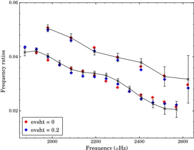
2000 2200 2400 2600 Frequency (µHz) 0.02 0.04 0.06 F re qu en cy ra ti os ovsht = 0 ovsht = 0.2
Fig. 6.Frequency separation ratios as a function of frequency for star A. Red diamonds correspond to our reference model computed without overshooting while blue diamonds correspond to our optimal model computed with overshooting (αov= 0.2). The observed ratios are shown
as connected points with errors.
method to obtain the best-fit model for the different sets of input physics considered.
We remind the reader that our reference model, labelled “Ref” in Table 5, was computed without overshooting, using the solar mixture of Asplund et al. (2009; hereafter AGSS09) and including microscopic diffusion. In order to check the con-sistency of the derived stellar parameters from our reference model, we then adopted the following input physics during the minimisation process:
– Model “Ovsht” computed assuming an overshoot parameter αov= 0.2.
– Model “GS98” computed using the solar mixture of Grevesse & Sauval(1998).
– Model “Nodiff” computed without microscopic diffusion. For each case, an optimal model was found by fitting the fre-quency ratios, as illustrated in Fig.6. The corresponding stellar parameters are listed in Table5.
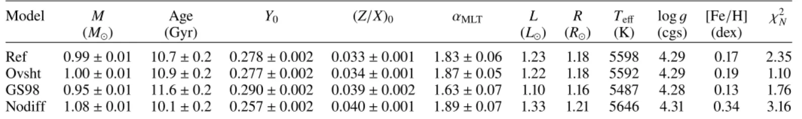
Based on the modelling results, the mass of star A appears to be in the range [0.95, 1.08] M . Unfortunately, the large
uncer-tainty on the orbital value of the mass, MA= 1.05+0.10−0.09M , does
not allow us to discard either of the models. In addition, we find the age of star A to be in the range 10.1–11.6 Gyr. As a result, the estimate of the age also suffers from a large uncertainty due to the physics used in the models. On the other hand, the inclusion of overshooting produces a better fit to the frequency ratios (see Fig.6). For this model, the derived values of the stellar parame-ters are in good agreement with those from our reference model, thereby reinforcing the results of this study.
We point out that further RV observations of HD 188753 are expected to provide much more stringent constraints on the stel-lar masses, which should help to disentangle the different input physics. In particular, the choice of the solar mixture requires a dedicated study, which is beyond the scope of this paper.
7. Conclusions
Using Kepler photometry, we report, for the first time, the detec-tion of solar-like oscilladetec-tions in the two brightest components of a close triple star system, HD 188753. We performed the seismic
Table 5. Derived fundamental parameters of star A for all the models using different input physics.
Model M Age Y0 (Z/X)0 αMLT L R Teff log g [Fe/H] χ2N
(M ) (Gyr) (L ) (R ) (K) (cgs) (dex)
Ref 0.99 ± 0.01 10.7 ± 0.2 0.278 ± 0.002 0.033 ± 0.001 1.83 ± 0.06 1.23 1.18 5598 4.29 0.17 2.35 Ovsht 1.00 ± 0.01 10.9 ± 0.2 0.277 ± 0.002 0.034 ± 0.001 1.87 ± 0.05 1.22 1.18 5592 4.29 0.19 1.10 GS98 0.95 ± 0.01 11.6 ± 0.2 0.290 ± 0.002 0.039 ± 0.002 1.63 ± 0.07 1.10 1.16 5487 4.28 0.13 1.76 Nodiff 1.08 ± 0.01 10.1 ± 0.2 0.257 ± 0.002 0.040 ± 0.001 1.89 ± 0.07 1.33 1.21 5646 4.31 0.34 3.16
Notes. Model “Ref” computed without overshooting, using the AGSS09 solar mixture and including microscopic diffusion (see Sect.5.1). Model “Ovsht” computed assuming an overshoot parameter αov= 0.2. Model “GS98” computed using the solar mixture ofGrevesse & Sauval(1998).
Model “Nodiff” computed without microscopic diffusion.
analysis of the two stars, providing accurate mode frequen-cies and reliable proxies of the stellar masses and ages. From the modelling, we also derived precise but model-dependent stellar parameters for the two oscillating components. In par-ticular, we found that the mean common age of the system is 10.8 ± 0.2 Gyr while the masses of the two seismic stars are MA= 0.99 ± 0.01 M and MBa= 0.86 ± 0.01 M . Furthermore,
we explored the impact on the derived stellar parameters of vary-ing the input physics of the models. For star A, the best-fit model was obtained by assuming an overshoot parameter of 0.2.
We also performed the first orbital analysis of HD 188753 that combines both the position and RV measurements of the system. For the wide pair, we derived the masses of the visual components and the parallax of the system, π= 21.9 ± 0.6 mas. In addition, we derived a precise mass ratio between both stars of the close pair, MBb/MBa= 0.767±0.006. We then found
individ-ual masses that are in good agreement with the modelling results. Finally, from the orbital analysis, we estimated the total mass of the system to be Msyst= 2.51+0.20−0.18M .
Combining the asteroseismic and astrometric observations of HD 188753 allowed us to better characterise the main features of this triple star system. For example, using the mass ratio of the close pair, we precisely determined the mass of the faintest star, MBb= 0.66 ± 0.01 M , from the seismic mass of its companion.
We then estimated the total seismic mass of the system to be Msyst = 2.51 ± 0.02 M , which agrees perfectly with the orbital
value. Injecting this latter into the Kepler’s third law leads to the best current estimate of the parallax for HD 188753, namely π = 21.9±0.2 mas. From our combined analysis, we also derived stringent limits on the relative inclination of the system. With a lower limit at 10.9◦± 1.5◦, we concluded that HD 188753 does not have a coplanar configuration.
In this work, we demonstrated that binaries and multiple stel-lar systems have the potential to constrain fundamental stelstel-lar parameters, such as the mass and the age. Further observa-tions using asteroseismology and astrometry also promise to improve our knowledge about the dynamical evolution of triple and higher-order systems. In this context, we stress the neces-sity to prepare catalogues of binaries and multiples for the future space missions TESS (Ricker et al. 2015) and PLATO (Rauer et al. 2014).
Acknowledgements.This paper includes data collected by the Kepler mission. Funding for the Kepler mission is provided by the NASA Science Mission directorate. The authors gratefully acknowledge the Kepler Science Operations Center (SOC) for reprocessing the short-cadence data that enabled the detection of the secondary seismic component. This research has made use of NASA’s Astrophysics Data System Bibliographic Services, the Washington Double Star Catalog maintained at the US Naval Observatory, the SIMBAD database, oper-ated at CDS, Strasbourg, France and the VizieR catalogue access tool, CDS, Strasbourg, France. The original description of the VizieR service was published
inOchsenbein et al.(2000). Finally, we also thank the anonymous referee for
comments that helped to improve this paper.
References
Alexander, D. R., & Ferguson, J. W. 1994,ApJ, 437, 879
Anderson, E. R., Duvall, Jr. T. L., & Jefferies, S. M. 1990,ApJ, 364, 699
Angulo, C., Arnould, M., Rayet, M., et al. 1999,Nucl. Phys. A, 656, 3
Appourchaux, T. 2014, inA Crash Course on Data Analysis in Asteroseismology, eds. P. L. Pallé, & C. Esteban,123
Appourchaux, T., Benomar, O., Gruberbauer, M., et al. 2012a, A&A, 537, A134
Appourchaux, T., Chaplin, W. J., García, R. A., et al. 2012b,A&A, 543, A54
Appourchaux, T., Antia, H. M., Benomar, O., et al. 2014,A&A, 566, A20
Appourchaux, T., Antia, H. M., Ball, W., et al. 2015,A&A, 582, A25
Armstrong, J. T., Mozurkewich, D., Vivekanand, M., et al. 1992,AJ, 104, 241
Asplund, M., Grevesse, N., Sauval, A. J., & Scott, P. 2009,ARA&A, 47, 481
Baglin, A., Auvergne, M., Barge, P., et al. 2006, inThe CoRoT Mission
Pre-Launch Status – Stellar Seismology and Planet Finding, eds. M. Fridlund,
A. Baglin, J. Lochard, & L. Conroy,ESA SP, 1306, 33
Baize, P. 1952,J. Obs., 35, 27
Baize, P. 1954,J. Obs., 37, 73
Baize, P. 1957,J. Obs., 40, 165
Ball, W. H., & Gizon, L. 2014a,A&A, 568, A123
Ball, W. H., & Gizon, L. 2014b,A&A, 569, C2
Baranne, A., Queloz, D., Mayor, M., et al. 1996,A&AS, 119, 373
Batten, A. H. 1973,Binary and Multiple Systems of Stars(Oxford, NY: Pergamon Press),International series of monographs in natural philosophy, 51
Böhm-Vitense, E. 1958,Z. Astrophys., 46, 108
Bouchy, F., & Carrier, F. 2002,A&A, 390, 205
Carrier, F., & Bourban, G. 2003,A&A, 406, L23
Chaplin, W. J., Kjeldsen, H., Christensen-Dalsgaard, J., et al. 2011,Science, 332, 213
Chaplin, W. J., Basu, S., Huber, D., et al. 2014,ApJS, 210, 1
Christensen-Dalsgaard, J. 1984, in Space Research in Stellar Activity and Variability, eds. A. Mangeney, & F. Praderie (Observatoire de Meudon),11
Christensen-Dalsgaard, J. 2008,Ap&SS, 316, 113
Couteau, P. 1967,J. Obs., 50, 41
Couteau, P. 1970,A&AS, 3, 51
Couteau, P., & Ling, J. 1991,A&AS, 88, 497
Couteau, P., Docobo, J. A., & Ling, J. 1993,A&AS, 100, 305
Creevey, O. L., Metcalfe, T. S., Schultheis, M., et al. 2017,A&A, 601, A67
Davies, G. R., Handberg, R., Miglio, A., et al. 2014,MNRAS, 445, L94
Davies, G. R., Chaplin, W. J., Farr, W. M., et al. 2015,MNRAS, 446, 2959
Davies, G. R., Silva Aguirre, V., Bedding, T. R., et al. 2016,MNRAS, 456, 2183
Eggenberger, A., Udry, S., Mazeh, T., Segal, Y., & Mayor, M. 2007,A&A, 466, 1179
ESA 1997,The HIPPARCOSand Tycho catalogues, Astrometric and photometric
star catalogues derived from the ESA HIPPARCOSSpace Astrometry Mission,
ESA SP, 1200
Fekel, Jr. F. C. 1981,ApJ, 246, 879
Formicola, A., Imbriani, G., Costantini, H., et al. 2004,Phys. Lett. B, 591, 61
Gilliland, R. L., Brown, T. M., Christensen-Dalsgaard, J., et al. 2010a,PASP, 122, 131
Gilliland, R. L., Jenkins, J. M., Borucki, W. J., et al. 2010b,ApJ, 713, L160
Grevesse, N., & Sauval, A. J. 1998,Space Sci. Rev., 85, 161
Griffin, R. F. 1967,ApJ, 148, 465
Gruberbauer, M., Guenther, D. B., MacLeod, K., & Kallinger, T. 2013,MNRAS, 435, 242
Hartkopf, W. I., & Mason, B. D. 2009,AJ, 138, 813
Hartkopf, W. I., McAlister, H. A., Mason, B. D., et al. 1997,AJ, 114, 1639
Hartkopf, W. I., Mason, B. D., McAlister, H. A., et al. 2000,AJ, 119, 3084
Hartkopf, W. I., Mason, B. D., & Worley, C. E. 2001a,AJ, 122, 3472
Hartkopf, W. I., McAlister, H. A., & Mason, B. D. 2001b,AJ, 122, 3480
Hastings, W. K. 1970,Biometrika, 57, 97
Heintz, W. D. 1975,ApJS, 29, 315
Heintz, W. D. 1978,Geophysics and Astrophysics Monographs,15
Heintz, W. D. 1980,ApJS, 44, 111
Heintz, W. D. 1990,ApJS, 74, 275
Heintz, W. D. 1998,ApJS, 117, 587
Holden, F. 1975,PASP, 87, 253
Holden, F. 1976,PASP, 88, 325
Horch, E., Ninkov, Z., van Altena, W. F., et al. 1999,AJ, 117, 548
Horch, E. P., Robinson, S. E., Meyer, R. D., et al. 2002,AJ, 123, 3442
Hough, G. W. 1899,Astron. Nachr., 149, 65
Huber, D., Ireland, M. J., Bedding, T. R., et al. 2012,ApJ, 760, 32
Huber, D., Silva Aguirre, V., Matthews, J. M., et al. 2014,ApJS, 211, 2
Iglesias, C. A., & Rogers, F. J. 1996,ApJ, 464, 943
Jenkins, J. M., Caldwell, D. A., Chandrasekaran, H., et al. 2010,ApJ, 713, L87
Kjeldsen, H., Bedding, T. R., & Christensen-Dalsgaard, J. 2008,ApJ, 683, L175
Kjeldsen, H., Christensen-Dalsgaard, J., Handberg, R., et al. 2010, Astron. Nachr., 331, 966
Konacki, M. 2005,Nature, 436, 230
Kozai, Y. 1962,AJ, 67, 591
Labeyrie, A., Bonneau, D., Stachnik, R. V., & Gezari, D. Y. 1974,ApJ, 194, L147
Lebreton, Y., & Montalbán, J. 2009, inIAU Symp., eds. E. E. Mamajek, D. R. Soderblom, & R. F. G. Wyse,258, 419
Lidov, M. L. 1962,Planet. Space Sci., 9, 719
Lindegren, L., Lammers, U., Bastian, U., et al. 2016,A&A, 595, A4
Lomb, N. R. 1976,Ap&SS, 39, 447
Lund, M. N., Silva Aguirre, V., Davies, G. R., et al. 2017,ApJ, 835, 172
Marques, J. P., Goupil, M. J., Lebreton, Y., et al. 2013,A&A, 549, A74
Mason, B. D., Hartkopf, W. I., Wycoff, G. L., et al. 2004,AJ, 128, 3012
Mason, B. D., Hartkopf, W. I., Raghavan, D., et al. 2011,AJ, 142, 176
Mazeh, T., Tsodikovich, Y., Segal, Y., et al. 2009,MNRAS, 399, 906
Mazumdar, A., Monteiro, M. J. P. F. G., Ballot, J., et al. 2014,ApJ, 782, 18
Metcalfe, T. S., Chaplin, W. J., Appourchaux, T., et al. 2012,ApJ, 748, L10
Metcalfe, T. S., Creevey, O. L., Do˘gan, G., et al. 2014,ApJS, 214, 27
Metcalfe, T. S., Creevey, O. L., & Davies, G. R. 2015,ApJ, 811, L37
Metropolis, N., Rosenbluth, A. W., Rosenbluth, M. N., Teller, A. H., & Teller, E. 1953,J. Chem. Phys., 21, 1087
Michaud, G., & Proffitt, C. R. 1993, inIAU Colloq. 137: Inside the Stars, eds. W. W. Weiss, & A. Baglin,ASP Conf. Ser., 40, 246
Miglio, A., Chiappini, C., Morel, T., et al. 2013,MNRAS, 429, 423
Miglio, A., Chaplin, W. J., Farmer, R., et al. 2014,ApJ, 784, L3
Morel, P., & Lebreton, Y. 2008,Ap&SS, 316, 61
Mosser, B., Michel, E., Belkacem, K., et al. 2013,A&A, 550, A126
Muller, P. 1955,J. Obs., 38, 221
Ochsenbein, F., Bauer, P., & Marcout, J. 2000,A&AS, 143, 23
Otí Floranes, H., Christensen-Dalsgaard, J., & Thompson, M. J. 2005,MNRAS, 356, 671
Planck Collaboration XVI. 2014,A&A, 571, A16
Pourbaix, D. 2008, inA Giant Step: from Milli- to Micro-arcsecond Astrometry, eds. W. J., Jin, I. Platais, & M. A. C. Perryman,IAU Symp., 248, 59
Pourbaix, D., & Boffin, H. M. J. 2016,A&A, 586, A90
Rauer, H., Catala, C., Aerts, C., et al. 2014,Exp. Astron., 38, 249
Ricker, G. R., Winn, J. N., Vanderspek, R., et al. 2015, J. Astron.Telesc. Instrum. Syst., 1, 014003
Rogers, F. J., & Nayfonov, A. 2002,ApJ, 576, 1064
Roxburgh, I. W. 2005,A&A, 434, 665
Roxburgh, I. W., & Vorontsov, S. V. 2003,A&A, 411, 215
Scargle, J. D. 1982,ApJ, 263, 835
Silva Aguirre, V., Davies, G. R., Basu, S., et al. 2015,MNRAS, 452, 2127
Söderhjelm, S. 1999,A&A, 341, 121
Sterzik, M. F., & Tokovinin, A. A. 2002,A&A, 384, 1030
Struve, F. G. W. 1837,Stellarum duplicium et multiplicium mensurae micro-metricae per magnum Fraunhoferi tubum annis a 1824 ad 1837 in Specula
Dorpatensi institutae(Academiae scientiarum caesareae petropolitanaeifique)
Tassoul, M. 1980,ApJS, 43, 469
Tohline, J. E. 2002,ARA&A, 40, 349
Tokovinin, A. A. 1980,Astronomicheskij Tsirkulyar, 1097, 3
Tokovinin, A. A. 1985,A&AS, 61, 483
Toonen, S., Hamers, A., & Portegies Zwart S. 2016, Comput. Astrophys. Cosmol., 3, 6
Trampedach, R., Stein, R. F., Christensen-Dalsgaard, J., Nordlund, Å., & Asplund, M. 2014,MNRAS, 445, 4366
van Biesbroeck G. 1918,AJ, 31, 169
van Biesbroeck G. 1927,Publications of the Yerkes Observatory, 5, 1
van Biesbroeck G. 1974,ApJS, 28, 413
van den Bos, W. H. 1959,ApJS, 4, 45
van den Bos, W. H. 1963,AJ, 68, 57
van Leeuwen, F. 2007,A&A, 474, 653
Verner, G. A., Elsworth, Y., Chaplin, W. J., et al. 2011,MNRAS, 415, 3539
Vogt, S. S., Allen, S. L., Bigelow, B. C., et al. 1994, inInstrumentation in
Astronomy VIII, eds. D. L., Crawford, & E. R. Craine,Proc. SPIE, 2198,
362
White, T. R., Bedding, T. R., Stello, D., et al. 2011,ApJ, 743, 161
White, T. R., Huber, D., Maestro, V., et al. 2013,MNRAS, 433, 1262
White, T. R., Benomar, O., Silva Aguirre, V., et al. 2017,A&A, 601, A82