Paquette, Gregory-Eaves and Beisner: Supporting Information
APPENDIX S1: Human impact index
Human impact was assessed using the land use types (urban, mines, agriculture, pasture, recent clear-cuts and natural landscape) in the watershed around each lake, and the classes of human impact were created based on the threshold values of Jenks natural break classification independently for each ecozone (Jenks & Caspall, 1971), so that the threshold values in HI classes is different among ecozone.
References
Jenks, G.F. & Caspall, F.C. (1971) Error on Choroplethic Maps: Definition,
Measurement, Reduction. Annals of the Association of American Geographers, 61, 217–244.
APPENDIX S2: Zooplankton sampling
At the deepest point of each lake, integrated water column zooplankton samples were collected using a 100µm mesh Wisconsin net (net radius = 10cm, length = 100cm), with a collection bucket (100µm) attached to the end. The net was hauled vertically from 1-m above the sediments to the lake surface. When lake depth was less than 6-m, additional vertical hauls from 1-m above sediments were taken to increase the volume sampled (to a minimum of 160L in total). Zooplankton were anesthetized with CO2 (Alka-Seltzer) and preserved with ethanol (final concentration approximately 70%). Samples were then stored at room temperature and sent to BSA Environmental Services (Ohio, U.S.A.) for species-level identification using a dissecting microscope (100x to 400x magnification). For each sample, at least 200 individuals of the most abundant species were counted, up to a total of 1000 individuals. Lakes wherein total abundance was < 100 individuals were removed from the dataset (n =10).
APPENDIX S3: Lake characteristics
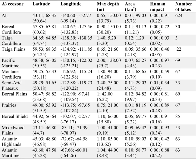
Table 1. Minimum; maximum and (mean) values of lake characteristics, as well as
number of lakes by ecozone (a) and continental divide (b). Regions are listed from west to east.
A) ecozone Latitude Longitude Max depth (m)
Area
(km2) Human impact Number of lakes
All 43.11; 68.35 (50.64) -140.60 ; -52.77 (-99.14) 0.65; 150.00 (13.79) 0.01; 99.03 (5.73) 0.00; 0.91 (0.22) 624 Boreal Cordillera 57.85; 63.81 (60.62) -140.67; -127.56 (-132.83) 0.90; 150.00 (30.20) 0.11; 91.13 (11.21) 0.00; 0.72 (0.05) 30 Taiga Cordillera 64.65; 64.85 (64.74) -138.39; -138.35 (-138.37) 1.40; 5.20 (3.30) 0.12; 1.29 (0.54) 0.00; 0.03 (0.02) 3 Taiga Plains 59.53; 68.35 (64.25) -134.92; -111.85 (-124.97) 0.65; 21.60 (4.28) 0.05; 35.66 (2.18) 0.00; 0.46 (0.05) 22 Pacific Maritime 48.38; 56.05 (50.55) -130.15; -122.02 (-125.21) 2.00; 138.00 (25.7) 0.07; 65.27 (4.43) 0.00; 0.97 (0.23) 69 Montane Cordillera 49.25; 55.33 (53.11) -126.92; -115.24 (-122.98) 1.80; 94.00 (16.20) 0.11; 68.65 (3.79) 0.00; 0.59 (0.10) 67 Semi-Arid Plateaux 49.29; 51.65 (50.18) -122.88; -119.23 (-120.22) 3.40; 75.00 (24.48) 0.11; 29.03 (4.73) 0.01; 0.34 (0.09) 33 Boreal Plains 50.47; 58.82 (53.68) -122.90; -97.41 (-109.54) 1; 42.00 (6.22) 0.12; 94.82 (9.97) 0.00; 0.81 (0.33) 69 Prairies 49.00; 53.92 (51.59) -113.75; -97.65 (-107.84) 0.75; 21.00 (4.10) 0.01; 81.19 (7.52) 0.00; 0.89 (0.48) 67 Boreal Shield 44.92; 56.64 (48.59) -102.07; -52.77 (-76.17) 1.10; 66.00 (15.80) 0.05; 69.77 (5.22) 0.00; 0.91 (0.16) 85 Mixedwood Plains 43.11; 46.80 (44.7) -83.11; -71.39. (-78.97) 1.00; 41.00 (9.19) 0.09; 69.42 (5.12) 0.00; 0.93 (0.34) 53 Atlantic Highlands 45.03; 48.80 (46.98) -72.67; -64.58 (-69.47) 1.10; 85.00 (13.62) 0.10; 99.03 (5.56) 0.00; 0.42 (0.12) 63 Atlantic Maritime 43.60; 47.58 (45.28) -67.66; -60.01 (-64.26) 1.04; 44.00 (8.48) 0.10; 58.77 (3.44) 0.00; 0.88 (0.22) 63
b) Contiental basin
Latitude Longitude Max depth (m)
Area
(km2) Human impact Number of lakes
All 43.11; 68.35 (50.64) -140.60 ; -52.77 (-99.14) 0.65; 150.00 (13.79) 0.01; 99.03 (5.73) 0.00; 0.91 (0.22) 624 Pacific Ocean 48.38; 63.81 (52.41) -140.67; -115.24 (-124.59) 0.90; 15.00 (22.60) 0.07; 91.13 (5.42) 0.00; 0.97 (0.14) 183 Arctic Ocean 53.45; 68.35 (59.37) -138.39; -111.16 (-122.89) 0.65; 73.00 (9.98) 0.05; 48.58 (4.53) 0.00; 0.80 (0.17) 66 Hudson Bay 47.84; 56.64 (51.72) -114.76; -74.22 (-103.04) 0.75; 42.00 (6.98) 0.01; 94.82 (9.02) 0.00; 0.89 (0.35) 142 Gulf of Mexico 49.07; 49.22 (49.14) -112.72; -105.85 (-109.29) 2.00; 2.50 (2.25) 4.06; 29.37 (16.71) 0.46; 0.55 (0.51) 2 Great Lakes-St. Lawrence 43.11; 52.41 (46.32) -83.31; -52.77 (-72.71) 1.00; 85.00 (13.04) 0.09; 99.03 (4.27) 0.00; 0.93 (0.23) 150 Atlantic Ocean 43.60; 48.80 (45.81) -69.55; -60.01 (-64.92) 1.04; 50.00 (10.44) 0.10; 67.74 (4.20) 0.00; 0.88 (0.19) 81
APPENDIX S5: Total biomass taxonomic and functional diversity
Table 2. Total biomass (µg d.w./L), taxonomic and functional diversity mean values ±
standard error by ecozone (a) and Continental basin (b). Significant p-values from the ANOVA are shown. Biggest values are highlighted in bold.
a) Ecozone Total biomass Shannon diversity Evenness Simpson diversity richness Total Rarefied richness Functional evenness Functional dispersion Functional richness
All 374.4 ± 51.1 1.03 ± 0.02 0.56 ± 0.01 0.52 ± 0.01 6.55 ± 0.10 5.60 ± 0.08 0.45 ± 0.01 0.15 ± 0.00 0.81 ± 0.02 Boreal Cordillera 88.6 ± 14.1 0.93 ± 0.05 0.68 ± 0.03 0.53 ± 0.02 4.17 ± 0.22 3.67 ± 0.16 0.57 ± 0.05 0.18 ± 0.01 0.47 ± 0.07 Taiga Plains 42.8 ± 11.0 0.88 ± 0.09 0.52 ± 0.04 0.46 ± 0.05 5.40 ± 0.42 4.55 ± 0.33 0.47 ± 0.05 0.12 ± 0.01 0.81 ± 0.11 Pacific Maritime 90.9 ± 28.2 0.97 ± 0.06 0.55 ± 0.03 0.49 ± 0.03 5.96 ± 0.25 5.23 ± 0.20 0.48 ± 0.03 0.13 ± 0.01 0.78 ± 0.06 Montane Cordillera 169.7 ± 22.83 0.93 ± 0.05 0.54 ± 0.03 0.49 ± 0.03 5.79 ± 0.25 5.13 ± 0.22 0.43 ± 0.03 0.13 ± 0.01 0.69 ± 0.06 Semi-Arid Plateaux 227.7 ± 70.1 0.86 ± 0.08 0.53 ± 0.04 0.46 ± 0.04 5.00 ± 0.23 4.52 ± 0.20 0.50 ± 0.05 0.13 ± 0.01 0.56 ± 0.07 Boreal Plains 869.2 ± 251.0 0.98 ± 0.06 0.50 ± 0.03 0.49 ± 0.03 7.10 ± 0.25 6.13 ± 0.21 0.43 ± 0.03 0.14 ± 0.01 1.05 ± 0.07 Prairies 1738.1 ± 341.89 0.94 ± 0.05 0.55 ± 0.03 0.49 ± 0.03 5.73 ± 0.21 5.05 ± 0.19 0.44 ± 0.03 0.14 ± 0.01 0.86 ± 0.07 Boreal Shield 89.1 ± 15.7 1.20 ± 0.05 0.59 ± 0.02 0.58 ± 0.02 7.99 ± 0.29 6.76 ± 0.25 0.46 ± 0.02 0.17 ± 0.01 0.81 ± 0.05 Mixedwood Plains 148.2 ± 51.3 1.24 ± 0.06 0.60 ± 0.02 0.60 ± 0.02 8.02 ± 0.28 6.59 ± 0.25 0.45 ± 0.03 0.17 ± 0.01 1.11 ± 0.07 Atlantic Highlands 117.3 ± 46.4 1.22 ± 0.05 0.59 ± 0.02 0.60 ± 0.02 7.90 ± 0.3 6.46 ± 0.25 0.43 ± 0.03 0.17 ± 0.01 0.89 ± 0.05 Atlantic Maritime 86.9 ± 11.7 0.90 ± 0.06 0.50 ± 0.03 0.45 ± 0.03 6.13 ± 0.28 5.15 ± 0.22 0.44 ± 0.03 0.12 ± 0.01 0.63 ± 0.05
b) Continental
basin Total biomass Shannon diversity Evenness Simpson diversity richness Total Rarefied richness Functional evenness Functional dispersion Functional richness
All 374.4 ± 51.1 1.03 ± 0.02 0.56 ± 0.01 0.52 ± 0.01 6.55 ± 0.1 5.6 ± 0.08 0.45 ± 0.01 0.15 ± 0 0.81 ± 0.02 Pacific Ocean 147.7 ± 18.8 0.91 ± 0.03 0.55 ± 0.02 0.48 ± 0.02 5.46 ± 0.14 4.85 ± 0.12 0.47 ± 0.02 0.13 ± 0.01 0.67 ± 0.04 Arctic Ocean 388.5 ± 217.2 0.95 ± 0.06 0.55 ± 0.03 0.49 ± 0.03 5.86 ± 0.27 5.01 ± 0.23 0.45 ± 0.03 0.14 ± 0.01 0.84 ± 0.07 Hudson Bay 1091.0 ± 185.1 1.04 ± 0.04 0.56 ± 0.02 0.52 ± 0.02 6.87 ± 0.21 5.94 ± 0.18 0.46 ± 0.02 0.15 ± 0.01 0.95 ± 0.04 Great Lakes-St. Lawrence 128.9 ± 27.4 1.20 ± 0.03 0.58 ± 0.01 0.59 ± 0.01 7.94 ± 0.18 6.55 ± 0.15 0.44 ± 0.02 0.16 ± 0.00 0.92 ± 0.04 Atlantic Ocean 79.5 ± 9.8 0.98 ± 0.05 0.53 ± 0.02 0.49 ± 0.02 6.4 ± 0.25 5.37 ± 0.21 0.44 ± 0.03 0.13 ± 0.01 0.67 ± 0.05 p-value <.0001 <.0001 NS <.0001 <2e-16 <.0001 NS <.0001 <.0001
APPENDIX S6: Total biomass by region
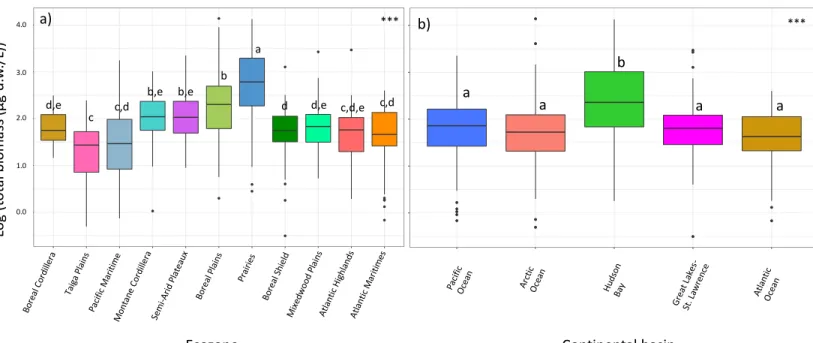
Figure 1: Total biomass means (± SE) across ecozones (a) and continental divides (b). Note that the y-axis scale varies between panels. Boxes that share the same letter are not significantly different. *p-value<0.05; **p-value<0.01; ***p-value<0.001
Bore al Co rdill era Taig a Pla ins Pacif ic M ariti me Mont ane Cor dille ra Sem i-Ar id P late aux Bore al P lain s Prai ries Bore al Shi eld Mixe dwoo d Pl ains Atla ntic High land s Atla ntic Mar itim es 0 1 2 3 4 Boreal Cordillera Taiga Plains Pacif ic Marit ime Mont ane Cordillera Semi-A rid Plat eaux Boreal Plains Prairies Boreal Shield Mixedwood Plains Atlant ic Highlands Atlant ic Marit ime Ecozone log(t ot al biomass) Pacif ic Oce an Arct ic Oce an Huds on Bay Grea t Lak es -St. L awre nce Atla ntic Oce an 0 1 2 3 4 Pacif ic O cean / Bering Sea Arct ic O cean Hudson Bay / Ungava Bay St. Lawrence / Labrador Sea Atlant ic O cean ContinentalDivide log(t ot al biomass) b a a a a Lo g ( to ta l b io m as s ( µg d. w ./ L) )
Ecozone Continental basin
*** a
b c
d,e c,d b,e b,e d d,e c,d,e c,d
*** a) b) 2.0 1.0 0.0 3.0 4.0
APPENDIX S7: Total biomass spatial distribution
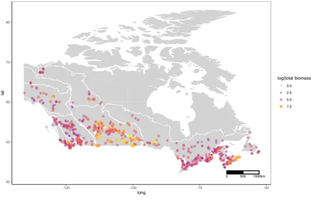
Figure 2: Heatmap of total crustacean zooplankton biomass (log transformed) by
ecozone. 0 500 1000km 40 50 60 70 80 -125 -100 -75 -50 long lat log(total biomass) 0.0 2.5 5.0 7.5
APPENDIX S8: Species rank-frequency occurrences
Figure 3: Rank-frequency occurrences of the 90 pelagic crustacean taxa collected in 624
lakes across Canada. Orange bars represent cladoceran species and blue bars represent copepod species.
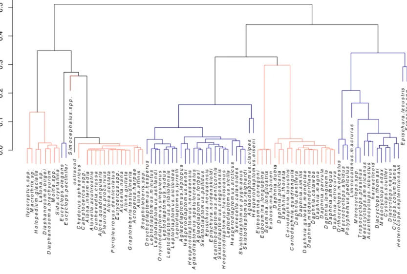
APPENDIX S9: Functional traits clustering
Functional group 1 included all S-filtration feeding type cladoceran herbivore species. Group 2 consisted only of littoral species, including C-filtration, raptorial and D-filtration feeding types. Group 3 was the largest functional group, consisting of
stationary-suspension calanoids. Group 4 consisted of pelagic herbivore species, including
Eubosmina spp. and Daphnia spp. Group 5 was composed of raptorial non-herbivore
species, including the most abundant cyclopoid, Diacyclops thomasi. Finally, group 6 contained only two species; the parasitic carnivore Ergasilus sp. and the current-cruiser feeder Epischura lacustris.
Figure 4: Cluster dendrogram based on functional traits of 92 zooplankton species based
on the Gower’s distance matrix calculated on their functional traits. Orange nods represent cladoceran species and blue bars represent copepod species.
APPENDIX S10: Taxonomic diversity by region Pacif ic Oce an Arct ic Oce an Huds on Bay Grea t Lake s-St . Lawr ence Atla ntic Oce an Bore al Co rdill era Taig a Pla ins Pacif ic M ariti me Mont ane Cor dille ra Sem i-Ar id P late aux Bore al P lain s Prai ries Bore al Shi eld Mixe dwoo d Pl ains Atla ntic High land s Atla ntic Mar itim es
Ecozone Continental divide
15.0 10.0 5.0 16.0 12.0 8.0 4.0 0.75 0.50 0.25 0.00 1.00 0.75 0.50 0.25 0.00 2.0 1.5 1.0 0.5 0.0 0.0 0.5 1.0 1.5 2.0 Pacif ic O cean / Bering Sea Arct ic O cean Hudson Bay / Ungava Bay St. Lawrence / Labrador Sea Atlant ic O cean Continental Divide S hannon diversit y 0.00 0.25 0.50 0.75 1.00 Pacif ic O cean / Bering Sea Arct ic O cean Hudson Bay / Ungava Bay St. Lawrence / Labrador Sea Atlant ic O cean Continental Divide E venness 0.00 0.25 0.50 0.75 Pacif ic O cean / Bering Sea Arct ic Ocean Hudson Bay / Ungava Bay St. Lawrence / Labrador Sea Atlant ic Ocean Continental Divide S impson diversit y 5 10 15 Pacif ic O cean / B ering Sea Arct ic O cean Hudson Bay / Ungava Bay St. Lawrence / Labrador Sea Atlant ic O cean Continental Divide Raref ied richness 0.00 0.25 0.50 0.75 1.00 Boreal Cordillera Taiga Plains Pacif ic Marit ime Mont ane Cordillera Semi-A rid Plat eaux Boreal Plains Prairies Boreal Shield Mixedwood Plains Atlant ic Highlands Atlant ic Marit ime Ecozone E venness Sh an no n di ve rs ity Ev en ne ss Si mp so n di ve rs ity Sp ec ie s ric hn es s Ra re fie d ric hn es s a) b) c) d) e) f) g) h) i) j) a a a a b a b b b a a a b b a a,b c . *** . *** . ** . *** . *** . *** . *** . *** . *** 0.0 0.5 1.0 1.5 2.0 Boreal Cordillera Taiga Plains Pacif ic Marit ime Mont ane Cordillera Semi-A rid Plat eaux Boreal Plains Prairies Boreal Shield Mixedwood Plains Atlant ic Highlands Atlant ic Marit ime Ecozone S hannon diversit y b a,b a,c a,c c a,b c c c c 0.00 0.25 0.50 0.75 Boreal Cordillera Taiga Plains Pacif ic Marit ime Mont ane Cordillera Semi-A rid Plateaux Boreal Plains Prairies Boreal Shield Mixedwood Plains Atlant ic Highlands Atlant ic Marit ime Ecozone S impson diversit y a,b a a,b b b 4 8 12 16 Boreal Cordillera Taiga Plains Pacif ic Marit ime Mont ane Cordillera Semi-A rid Plat eaux Boreal Plains Prairies Boreal Shield Mixedwood Plains Atlant ic Highlands Atlant ic Marit ime Ecozone S pecies richness c,d a,d a a b,c b,c c c a c,d b 4 8 12 16 Pacif ic O cean Arct ic O cean Hudson Bay Great Lakes-S t. Lawrence Atlant ic O cean Continental Divide S pecies richness a a,b b c b 5 10 15 Boreal Cordillera Taiga Plains Pacif ic Marit ime Mont ane Cordillera Semi-A rid Plateaux Boreal Plains Prairies Boreal Shield Mixedwood Plains Atlant ic Highlands Atlant ic Marit ime Ecozone Raref ied richness c b a,d a a a b,c b,c,d c,d c c . *** . *** . *** . *** . ***
Figure 5: Taxonomic diversity indices: Shannon diversity (a,b), evenness(c,d), simpson
diversity(e,f), richness (g,h), rarefied richness (i,j) means (± SE across ecozones and continental basins respectively). Note that the y-axis scale varies between panels. Boxes that share the same letter are not significantly different. *p-value<0.05; **p-value<0.01; ***p-value<0.001
APPENDIX S11: Functional diversity by region
Figure 6: Functional diversity indices: functional evenness (a,bl), functional dispersion
(c,d) and functional richness (e,f) means (± SE across ecozones and continental basins respectively). Note that the y-axis scale varies between panels. Boxes that share the same letter are not significantly different. *p-value<0.05; **p-value<0.01; ***p-value<0.001
Pacif ic Oce an Arct ic Oce an Huds on Bay Grea t Lake s-St . Lawr ence Atla ntic Oce an Bore al Co rdill era Taig a Pla ins Pacif ic M ariti me Mont ane Cor dille ra Sem i-Arid Pla teau x Bore al P lain s Prai ries Bore al S hiel d Mixe dwoo d Pl ains Atla ntic High land s Atla ntic Mar itim es
Ecozone
Continental divide
0.00 0.25 0.50 0.75 1.00 Pacif ic O cean / Bering Sea Arct ic O cean Hudson Bay / Ungava Bay St. Lawrence / Labrador Sea Atlant ic O cean Continental Divide F unct ional evenness 0.0 0.1 0.2 0.3 Pacif ic O cean / Bering Sea Arct ic O cean Hudson Bay / Ungava Bay St. Lawrence / Labrador Sea Atlant ic O cean Continental Divide F unct ional dispersion 0 1 2 Pacif ic O cean / Bering Sea Arct ic O cean Hudson Bay / Ungava Bay St. Lawrence / Labrador Sea Atlant ic O cean Continental Divide F unct ional richness 0.00 0.25 0.50 0.75 1.00 Boreal Cordillera Taiga Plains Pacif ic Marit ime Mont ane Cordillera Semi-A rid Plat eaux Boreal Plains Prairies Boreal Shield Mixedwood Plains Atlant ic Highlands Atlant ic Marit ime Ecozone F unct ional evenness 0.0 0.1 0.2 0.3 Boreal Cordillera Taiga Plains Pacif ic Marit ime Mont ane Cordillera Semi-A rid Plat eaux Boreal Plains Prairies Boreal Shield Mixedwood Plains Atlant ic Highlands Atlant ic Marit ime Ecozone F unct ional dispersion 2.0 1.0 0.0 0.3 0.2 0.1 0.0 1.00 0.75 0.50 0.25 0.00
Fu
nc
tio
na
l e
ve
nn
es
s
Fu
nc
tio
na
l d
is
pe
rs
io
n
Fu
nc
tio
na
l r
ic
hn
es
s
a) c) e) b) d) f) a b,c a a,c a b a a b b b a a***
***
***
***
0 1 2 Boreal Cordillera Taiga Plains Pacif ic Marit ime Mont ane Cordillera Semi-A rid Plat eaux Boreal Plains Prairies Boreal Shield Mixedwood Plains Atlant ic Highlands Atlant ic Marit ime Ecozone F unct ional richness a c,d b,c b,c b,d b a,c a,c a,c a,c***
APPENDIX S12: Spatial patterns in alpha diversity
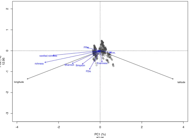
Figure 7: PCA ordination plot (scaling 2) of lake longitude and latitude with alpha
diversity indices plotted passively. Only lakes where all diversity indices could be calculated are illustrated (n=613)
-4 -2 0 2 4 -3 -2 -1 0 12 PCA - scaling 2 PC1 (%) 87.05 P C2 (%) 12. 95 latitude longitude
Shannon Simpson Evenness
richness rarefied richness
FRic
FEve,
APPENDIX S13: Total taxonomic beta diversity
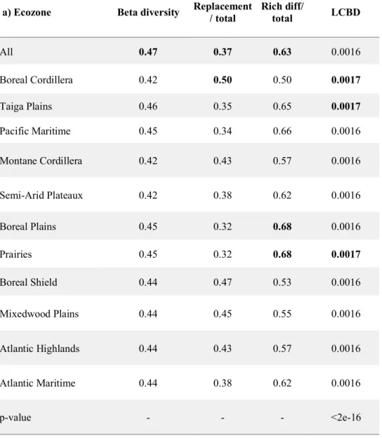
Table 3: Total taxonomic beta diversity, replacement and richness difference
components, as computed with beta() and LCBD values as computed with beta.div() by ecozone (a) and continental divide (b). Significant p-values from the ANOVAs are shown. Biggest values are highlighted in bold.
a) Ecozone Beta diversity Replacement / total Rich diff/ total LCBD
All 0.47 0.37 0.63 0.0016 Boreal Cordillera 0.42 0.50 0.50 0.0017 Taiga Plains 0.46 0.35 0.65 0.0017 Pacific Maritime 0.45 0.34 0.66 0.0016 Montane Cordillera 0.42 0.43 0.57 0.0016 Semi-Arid Plateaux 0.42 0.38 0.62 0.0016 Boreal Plains 0.45 0.32 0.68 0.0016 Prairies 0.45 0.32 0.68 0.0017 Boreal Shield 0.44 0.47 0.53 0.0016 Mixedwood Plains 0.44 0.45 0.55 0.0016 Atlantic Highlands 0.44 0.43 0.57 0.0016 Atlantic Maritime 0.44 0.38 0.62 0.0016 p-value - - - <2e-16
b) Continental basin diversity Beta Replacement / total Rich diff/ total LCBD
All 0.47 0.37 0.63 0.0016
Pacific Ocean 0.45 0.38 0.62 0.0016
Arctic Ocean 0.46 0.36 0.64 0.0017
Hudson Bay 0.46 0.30 0.70 0.0016
Great Lakes-St. Lawrence 0.44 0.46 0.54 0.0016
Atlantic Ocean 0.43 0.37 0.63 0.0016
APPENDIX S14: Total functional beta diversity
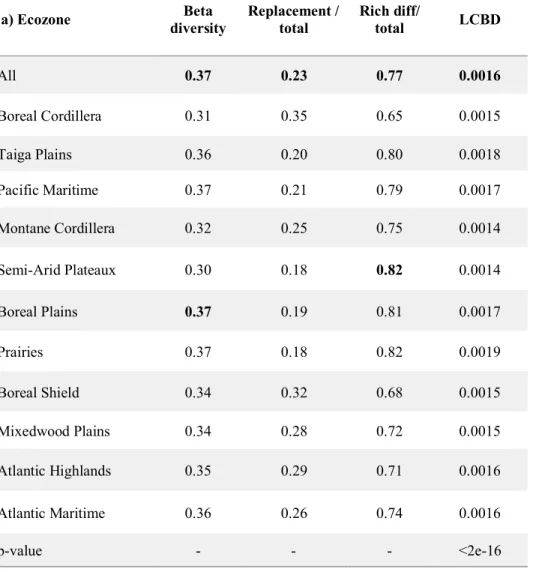
Table 4: Total functional beta diversity, replacement (turnover) and richness difference
(nestedness-resultant) components, as computed with beta() and LCBD values as computed with LCBD.comp() by ecozone (a) and continental divide (bSignificant p-values from the ANOVAs are shown. Biggest p-values are highlighted in bold.
a) Ecozone diversity Beta Replacement / total Rich diff/ total LCBD
All 0.37 0.23 0.77 0.0016 Boreal Cordillera 0.31 0.35 0.65 0.0015 Taiga Plains 0.36 0.20 0.80 0.0018 Pacific Maritime 0.37 0.21 0.79 0.0017 Montane Cordillera 0.32 0.25 0.75 0.0014 Semi-Arid Plateaux 0.30 0.18 0.82 0.0014 Boreal Plains 0.37 0.19 0.81 0.0017 Prairies 0.37 0.18 0.82 0.0019 Boreal Shield 0.34 0.32 0.68 0.0015 Mixedwood Plains 0.34 0.28 0.72 0.0015 Atlantic Highlands 0.35 0.29 0.71 0.0016 Atlantic Maritime 0.36 0.26 0.74 0.0016 p-value - - - <2e-16
b) Continental
basin Beta diversity Replacement / total Rich diff/ total LCBD
All 0.38 0.23 0.77 0.0016 Pacific Ocean 0.36 0.22 0.78 0.0016 Arctic Ocean 0.37 0.22 0.78 0.0016 Hudson Bay 0.39 0.17 0.83 0.0017 Great Lakes-St. Lawrence 0.35 0.30 0.70 0.0015 Atlantic Ocean 0.36 0.26 0.74 0.0016 p-value - - - 1.3e-07
APPENDIX S15: Local contribution to diversity (LCBD) by region
Figure 8: taxonomic (a,b) and functional (c,d) LCBD means (± SE across ecozones and
continental divides respectively). Note that the y-axis scale varies between panels. Boxes that share the same letter are not significantly different. *p-value<0.05; **p-value<0.01; ***p-value<0.001 Pacif ic Oce an Arct ic Oce an Huds on Bay Grea t Lake s-St . Lawr ence Atla ntic Oce an Bore al Co rdill era Taig a Pla ins Pacif ic M ariti me Mont ane Cor dille ra Sem i-Ar id P late aux Bore al P lain s Prai ries Bore al S hiel d Mixe dwoo d Pl ains Atla ntic High land s Atla ntic Mar itim es
Ecozone
Continental basin
0.0010 0.0015 0.0020 0.0025 Pacif ic O cean / B ering Sea Arct ic O cean Hudson Bay / Ungava Bay St. Lawrence / Labrador Sea Atlant ic O cean Continental Divide LCB DF
Fu
nc
tio
na
l L
CB
D
0.0015 0.0020 0.0025 c) d) a a a b***
0.00125 0.00150 0.00175 0.00200 Pacif ic O cean / B ering Sea Arct ic O cean Hudson Bay / Ungava Bay St. Lawrence / Labrador Sea Atlant ic O cean Continental Divide LCB D 0.00125 0.00150 0.00175 0.00200 Boreal Cordillera Taiga Plains Pacif ic Marit ime Mont ane Cordillera Semi-A rid Plat eaux Boreal Plains Prairies Boreal Shield Mixedwood Plains Atlant ic Highlands Atlant ic Marit ime Ecozone LCB DTa
xo
no
m
ic
L
CB
D
0.0013 0.00175 0.0020 a) b) a a b,d c a,d c b,c b,c b,c b,c b,c,d a,c a b c a,c***
***
0.00150 0.00125 0.0010 0.0015 0.0020 0.0025 Boreal Cordillera Taiga Plains Pacif ic Marit ime Mont ane Cordillera Semi-A rid Plat eaux Boreal Plains Prairies Boreal Shield Mixedwood Plains Atlant ic Highlands Atlant ic Marit ime Ecozone LCB DF a,b d a b b,d b,c a a,c a,c***
a,b a,bAPPENDIX S16: Species contribution to diversity (SCBD) Species SCBD Daphnia pulicaria 0.15 Bosmina longirostris 0.07 Leptodiaptomus minutus 0.06 Skistodiaptomus oregonensis 0.06 Mesocyclops edax 0.06 Daphnia.galeata mendotae 0.05 Diacyclops thomasi 0.04 Leptodiaptomus sicilis 0.03 Holopedium glacialis 0.03 Leptodiaptomus pribilofensis 0.03 Daphnia dentifera 0.03 Tropocyclops prasinus 0.03 Acanthocyclops robustus 0.02 Daphnia catawba 0.02 Aglaodiaptomus leptopus 0.02 Daphnia retrocurva 0.02 Leptodiaptomus siciloides 0.02 Epischura lacustris 0.02 Acanthodiaptomus denticornis 0.02 Heterocope septentrionalis 0.02 Diaphanosoma brachyurum 0.02 Leptodiaptomus nudus 0.01 Cyclops columbianus 0.01 Diaphanosoma birgei 0.01 Cyclops scutifer 0.01 Eubosmina longispina 0.01 Chydorus sphaericus 0.01
Table 5: Species with SCBD larger than mean SCBD, as computed with