HAL Id: hal-02595635
https://hal.inrae.fr/hal-02595635
Submitted on 15 May 2020HAL is a multi-disciplinary open access archive for the deposit and dissemination of sci-entific research documents, whether they are pub-lished or not. The documents may come from teaching and research institutions in France or abroad, or from public or private research centers.
L’archive ouverte pluridisciplinaire HAL, est destinée au dépôt et à la diffusion de documents scientifiques de niveau recherche, publiés ou non, émanant des établissements d’enseignement et de recherche français ou étrangers, des laboratoires publics ou privés.
Tracking the uncertainty in streamflow prediction
through a hydrological forecasting system
T. van Pham
To cite this version:
T. van Pham. Tracking the uncertainty in streamflow prediction through a hydrological forecasting system. Environmental Sciences. 2011. �hal-02595635�
UNIVERSITY OF TWENTE.
Tracking the uncertainty in
streamflow prediction through a
hydrological forecasting
system
August 2011
Trang Van Pham
Internal supervisors: University of Twente Dr. M.S. Krol
Associate Professor | [email protected]
Dr.Ir. M.J. Booij
Assistant Professor | [email protected]
University of Twente
Faculty of Engineering Technology Department of Water Engineering and Management P.O. Box 217 7500AE Enschede The Netherlands External supervisor: Cemagref Dr. M.H. Ramos Researcher | [email protected] Cemagref Antony Research Unit HBAN
1, rue Pierre-Gilles de Gennes CS 10030 92761 Antony Cedex France CemOA : archive ouverte d'Irstea / Cemagref
Summary
A flood forecasting system is a complex system which consists of many different components and each of these components can contain, to some extent, an uncertainty. Studying the uncertainties in flood forecasting, quantifying and propagating them through the system can help to gain more information about the different sources of uncertainty that may affect the forecasts. This information can later be added to the forecasts to improve their quality. These issues bring several challenges to the study of flow forecasting uncertainty: firstly, what is the impact of different sources of uncertainty on the quality of flood? Secondly, forecasts among all sources of uncertainty that stem from different components of the system, which sources significantly affect flood forecasts? Thirdly, which methods can be used to efficiently quantify and propagate those uncertainties through a forecasting model? Finally, which measures should be used to evaluate the uncertainty quantification and their impact on the quality of the forecasts? The aims of this research is to quantify and propagate the different kinds of uncertainty sources which play a role in flood forecasting; and to investigate methods to assess the quantified uncertainties and proper measures to evaluate the uncertainty quantification.
In this research, the GRPE forecasting system, an ensemble prediction system based on the lumped GRP hydrologic model, is applied to three catchments in France. The uncertainties from precipitation data (input precipitation which is used for flow simulation and forecast precipitation used for flow forecasting), hydrological initial conditions (discharge data) and model parameters, which are acknowledged as important sources of uncertainty in hydrological modelling and forecasting, are studied. They are individually quantified and then propagated together through the forecasting system with an experimental approach by multiplying the simulations. The model structure uncertainty is not considered in the scope of this research.
Methods for uncertainty quantification are defined and applied to each source of uncertainty. Two ensemble prediction systems from ECMWF and Météo-France are used to account for the forecast precipitation uncertainty for lead times from 1 to 9 days. For the uncertainty of input precipitation data, geo-statistical simulations of spatially averaged rainfall, conditioned on point data, and available for one study catchment, are chosen to provide the multiple statistical realizations of daily spatial rainfall fields over the study area. The hydrologic initial condition uncertainty is quantified by using an ensemble of discharges to update the state of the routing reservoir of the forecasting model. These discharges are retrieved from the analysis of uncertainties affecting the rating curves of each study catchment. Ten different periods of data, with the length of 5 years each, are selected to calibrate the model and thus to account for calibration period uncertainty. Finally, the Generalized Likelihood Uncertainty Estimator (GLUE) method is alternatively used to quantify the parameterization uncertainty. This is done by taking a large number of 125.000 sets of parameters to find the confidence intervals. To assess the results of uncertainty quantification, two probabilistic evaluation measures, the Brier (Skill) Score and the reliability diagram, are employed. In addition, confidence intervals of the forecasts are used to visualize the outcome of the research.
CemOA
: archive
ouverte
d'Irstea
The results show that input precipitation uncertainty does not have noticeable impact on the forecast output. This may be due to the method used to quantify the uncertainties from this source, which may be inappropriate to correctly capture them. For the catchments studied, this source of uncertainty can, therefore, be neglected when propagating different sources of uncertainty through the system. The other sources of uncertainty show large impacts on flow forecasts. Initial condition uncertainty shows large impacts for small lead times (up to 2 days). After that, forecast precipitation uncertainty has the largest impact; this impact is more significantly pronounced at high lead times. Depending on the catchment, parameter uncertainty can have more impact if it is evaluated from the variation of the calibration period or from the GLUE method.
Based on the results of this research, and on the catchments and methods investigated, it is recommended to take into consideration the uncertainty of forecast precipitation, initial condition and model parameters in flood forecasting. There are different ways to account for parameter uncertainty, but the proposed approach of using different calibration periods proved to be a simple method but able to improve the quality of the forecast outputs.
CemOA
: archive
ouverte
d'Irstea
Preface
This thesis report is the final product of my master programme on Civil Engineering and Management with the specialisation on Water Engineering and Management at University of Twente, the Netherlands. This was done partially in University of Twente and partially in Cemagref Antony, France.
I would like to express my appreciation to my supervisors Dr. Martijn Booij and Dr. Maarten Krol, who gave me very helpful advice during the research time. Special thanks go to Dr. Maria-Helena Ramos, my supervisor in Cemagref, thank you for your great help academically and personally during the time I worked in France.
I would like to also acknowledge here the work of Benjamin Renard and Etienne Leblois from Cemagref Lyon, France on rating curve and spatial average precipitation uncertainty quantification. I acknowledge Météo-France for the SAFRAN data archive and the PEARP ensemble forecasts, European Centre of Medium Range Weather Forecasting for the ensemble prediction system forecasts and the French MEEDM (Ministère de l’Ecologie, de l’Energie, du Développement durable et de la Mer) for the streamflow data.
Thanks to all of my colleagues in Cemagref, you were very friendly and helped me a lot during my four months stay there. Special thanks go to my Vietnamese dear friends in Twente, many of them are here, many of them are not here anymore, but they always support me, give me help when I need without any hesitation. Without you all, it would be impossible for me to have such a great and comfortable time here.
I would like to express my love and appreciation to my parents for their love and support and for the fact that they gave me this great opportunity in my life.
Last but not least, I want to thank my boy friend, Ali Riza Konuk, thank you so much for your incredible support and love. It was a big motivation for me to complete this research.
Enschede, August 2011 Trang Van Pham
CemOA
: archive
ouverte
d'Irstea
Table of Contents
1 INTRODUCTION ... 6
1.1 MOTIVATION ... 6
1.2 UNCERTAINTY ANALYSIS IN FLOOD FORECASTING ... 7
1.2.1 Quantification of uncertainties in flow forecasting ... 8
1.2.2 Propagation of uncertainties in flow forecasting ... 11
1.2.3 Evaluation of forecast uncertainty ... 12
1.3 PROBLEM DEFINITION... 13
1.4 OBJECTIVE AND RESEARCH QUESTIONS ... 13
1.5 REPORT OUTLINE ... 14
2 STUDY MATERIALS ... 15
2.1 STUDY AREAS... 15
2.2 OBSERVED PRECIPITATION AND DISCHARGE DATA ... 16
2.3 FORECASTING SYSTEM AND GRP MODEL ... 17
2.3.1 Forecasting system ... 17
2.3.2 GRP model structure and parameters ... 17
2.3.3 Calibration, validation and forecast in the GRPE forecasting system ... 18
3 METHODS ... 20
3.1 IDENTIFYING UNCERTAINTY SOURCES ... 20
3.1.1 Initial identification of uncertainty sources ... 20
3.1.2 Determination of uncertainty source importance ... 23
3.2 QUANTIFYING THE IMPACT OF INDIVIDUAL UNCERTAINTY ON FLOOD FORECAST ... 25
3.2.1 Input precipitation uncertainty ... 25
3.2.2 Forecast precipitation uncertainty ... 27
3.2.3 Initial condition uncertainty ... 29
3.2.4 Parameter uncertainty ... 32
3.2.5 Individual uncertainty quantification tests ... 41
3.3 PROPAGATING UNCERTAINTY THROUGH THE FORECAST SYSTEM ... 41
3.4 EVALUATING THE FORECAST OUTPUTS ... 45
3.4.1 Reliability diagram ... 45
3.4.2 Brier Score ... 47
3.4.3 Confidence intervals ... 49
4 RESULTS AND DISCUSSIONS ... 50
4.1 INDIVIDUAL IMPACT OF THE UNCERTAINTY SOURCES ... 50
4.2 COMBINED IMPACTS OF THE UNCERTAINTY SOURCES ... 52
4.2.1 Uncertainty of forecast precipitation and initial condition ... 53
4.2.2 Uncertainty of model parameter ... 58
4.2.3 Accounting for all sources of uncertainty... 63
4.3 DISCUSSIONS ... 65
5 CONCLUSIONS AND RECOMMENDATIONS ... 67
5.1 CONCLUSIONS ... 68 5.2 RECOMMENDATIONS ... 69 6 REFERENCES ... 70 APPENDIX ... 74 CemOA : archive ouverte d'Irstea / Cemagref
1
Introduction
1.1
Motivation
Flood is a major natural disaster in many countries all over the world. The consequences of flooding can be enormous in term of property loss and fatalities. According to the European Commission (2011), in Europe, there were more than 100 major damaging floods only in a period of three years between 1998 and 2002, which represents, on average, more than 30 floods per year. Among those, there was the catastrophic flood along the Danube and Elbe rivers in 2002; which was a 100 year-flood that caused billions of Euros of damage in many countries in Eastern Europe (BBC, 2002). Since 1998, floods have caused some 700 fatalities, the displacement of about half a million people and at least 25 billion Euros in insured economic losses in Europe (European Commission, 2011).
Flood forecasting is one of the solutions to prevent the consequences of flooding, as it can provide information on whether a potential flood might happen in the long or short term future. Based on the flood forecasts issued, flood warning, prevention and evacuation solutions can be implemented. According to the American Meteorological Society Glossary (American Meteorological Society, 2011), "flood forecasting is the use of real-time precipitation and streamflow data in rainfall-runoff and streamflow routing models to forecast flow rates and water levels for periods ranging from a few hours to days ahead, depending on the size of the watershed or river basin".
However, telling something that might happen in the future is not an easy task as the future itself is anyway something we cannot know at this moment and hence uncertain. Lack of knowledge about the physical processes involved in flooding and the data used, as well as inherent unpredictability of severe events can lead to uncertainties in the forecasts. Errors in the forecasting of flood may lead to (Smith and Ward, 1998):
- under-preparation and therefore to otherwise avoidable damage (if the forecast stage is too low and/or the forecast timing of inundation is late), or
- over-preparation, unnecessary expense and anxiety, and to a subsequent loss of credibility (if the forecast stage is too high and/or the forecast timing of inundation is premature).
A typical example of how not taking into account the errors in flood prediction can lead to severe consequences is reported by Krzysztofowicz (2001) for the flood event of Spring 1997 on the Red River in the Grand Forks, North Dakota, USA. The estimated 15 meter flood crest, with no uncertainty bounds associated to this value, led city officials and residents to prepare for the future event as if this estimate were a perfect forecast. However, the forecast actually seriously underestimated the event and the actual flood crest was of 16.5 meters, overtopping the dikes, and inundating 80% of the city which forced almost the total evacuation of its citizens.
CemOA
: archive
ouverte
d'Irstea
Therefore, it can be seen that assessing uncertainties in flood forecasting is a very crucial issue; especially in a well-developed world nowadays where a great number of sophisticated infrastructure systems were built or are being built, which makes people much more vulnerable to natural disasters. Understanding the uncertainties that exist in the flood forecasting chain will help people to be aware of them and be better prepared for the future events. Furthermore, uncertainty assessment also helps scientists to find innovative solutions to quantify and reduce those uncertainties. Besides the forecast quality is affected by the lack of knowledge on uncertainty, and therefore, the quantification of uncertainty also contributes to adding more information/knowledge into the flow forecasting procedure to improve the quality of the forecasts. Forecasts can thus become more reliable in terms of probability, or/and more accurate in terms of magnitude.
In the coming section, a general overview of uncertainty analysis in streamflow prediction is presented. The focus is on the identification, quantification, propagation and evaluation of flow forecasting uncertainty.
1.2
Uncertainty analysis in flood forecasting
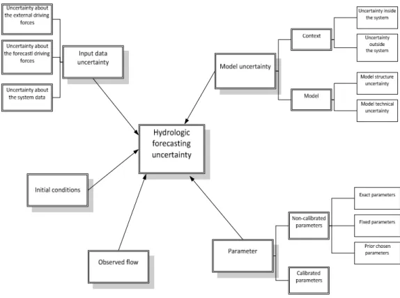
There are different sources of uncertainty that might affect flow forecasting. In the context of flood forecasting, Maskey et al. (2004) classified the sources of uncertainty as model uncertainty, input uncertainty, model parameter uncertainty, natural and operational uncertainty. Except the last source of uncertainty, which originates from the nature and the operation and is not related to the forecasting model, others come from the different components of the flow forecasting model as illustrated in Figure 1. The input data for a flow forecasting model have two kinds, input for flow simulation and forecasting; uncertainty of the input data can arise from both of these sources. Other source of uncertainty that is not mentioned by Maskey et al. (2004) is initial condition uncertainty which comes from the inappropriate estimation of the initial state for flow forecasting. All of these sources of uncertainty can propagate into the forecast outcome and cause the uncertainty of the flow forecasting. In addition, the forecasts are often verified against a reference which is often taken as the observed discharge. However, as the measurement of discharge is not error free, uncertainty can also stem from this component.
Figure 1: Main components of a typical hydrological forecasting chain
CemOA
: archive
ouverte
d'Irstea
1.2.1
Quantification of uncertainties in flow forecasting
Many studies can be found in the literature that study one or some of the uncertainty sources mentioned above. Most of them show that taking into consideration the uncertainties would improve the reliability of the forecast.
Using the ensemble prediction systems (EPS) is a popular approach to assess the uncertainty in flow forecasting due to precipitation forecast uncertainty. Many published literature, which have used EPS, are listed in Cloke and Pappenberger (2009). The authors also showed the attractiveness and potential of using ensemble prediction systems (EPS) to account for uncertainty from the forecast of precipitation in flow forecasting. Ensemble forecasts of precipitation take into account the uncertainties in the atmospheric state and initial conditions, as well as the limitation of the representation of the physical process in weather forecasting. As a result, a set of possible future states of the atmosphere is provided. This uncertainty can be then propagated through flood forecasting system to produce an ensemble prediction of flow as shown in Figure 2. By reviewing published literature and based on their results, the authors demonstrated that using the precipitation ensembles in flood prediction can increase the capability of issuing the successful flood warnings. Moreover, the ensemble predictions help to add additional useful information to the deterministic forecast which is the best estimation of the future event.
Figure 2: Ensemble hydrographs for a flood event predicted for each ensemble forecast of precipitation (Cloke and Pappenberger, 2009) CemOA : archive ouverte d'Irstea / Cemagref
Pappenberger et al. (2005) cascaded the uncertainty of rainfall from medium range weather forecasts into flow forecasts using the ensemble prediction system from the European Centre of Medium Range Weather Forecasting (ECMWF). The authors also concluded that the errors in rainfall forecasts had a strong influence on the forecast flows.
He et al. (2009) used not only one, but multiple ensemble weather predictions from various weather centres to cascade the uncertainty of precipitation forecast through a flow forecasting model. The best six sets of model parameters were selected, to account for parameter uncertainty, and combined with 216 forecasts members to form 6*216 ensemble forecast discharges. The paper shows that forecast precipitation uncertainty dominates and propagates through the forecast chain, implying the importance of accounting for this precipitation uncertainty in flow forecasting.
Mascaro et al. (2010) also admitted the important contribution of evaluating the propagation of errors associated with ensemble precipitation forecasts into the ensemble streamflow to uncertainty reduction in flow forecasting. In their paper, the authors generated and verified three different sets of ensemble streamflow forecasts by using three ensembles of precipitation forecasts.
Concerning uncertainty from input data, in Renard et al. (2010), the authors stated that the traditional calibration methods in hydrological modelling assume all observed inputs are error free, and therefore there is no input uncertainty which is obviously not realistic. For that reason, in their papers, the Bayesian total error analysis (BATEA) framework was used to assess the uncertainty of input data. The outcome of their work proves that ignoring input uncertainty can significantly degrade the inference of flow prediction, and hence, this source of uncertainty should be considered in hydrologic prediction.
Berthet et al. (2009) focused on investigating the impact of soil moisture initial conditions on the performance of flood forecasting models and finding the level of importance of accounting for the initial condition uncertainty in flood forecasting. They applied different methods of forecast initialization (updating) and compared the prediction errors obtained from those tests to find the best approach to deal with the initial condition in a flood forecasting model. Their study shows that different methods of initialization have different impacts on the forecast outcome and there is an optimum mode for initializing. Because of the large and varied data that were used, the authors stated that the results were probably not catchment-dependent. It is also suggested in the paper that the same results achieved for the model studied could be found for many other forecasting models.
Many studies on hydrological simulation and prediction quantify parameter uncertainty using the Generalized Likelihood Uncertainty Estimator (GLUE) proposed by Beven and Binley (1992) (see Pappenberger et al. (2004), Pappenberger et al. (2005), Larsbo and Jarvis (2005), Xiong and O’Connor (2008), Jin et al. (2010), etc.). The main idea of the GLUE method is rejecting the concept of an optimum model and parameter set, and assuming that prior to input of data into a model, all model structures and parameter sets have an equal likelihood of being acceptable. By using a number of parameter sets or model structure, series of equally
CemOA
: archive
ouverte
d'Irstea
likely simulations can be obtained. After the data for a particular case being considered, the model structures or parameter sets can be attributed as non-behavioural or behavioural depending on the likelihood threshold that is defined by the user. Confidence intervals can be defined for the flow simulations or forecasts using the cumulative distribution function of discharge weighted by the likelihood value. Larsbo and Jarvis (2005) recommended GLUE a suitable method of parameter uncertainty estimation for prediction. Pappenberger et al. (2004) did a study in the Meuse river basin in the Netherlands and Belgium using the GLUE method. A large number of 6632 runs were performed but none of the simulations was found as behavioural. It is concluded in the paper that "uncertainty analysis should be compulsory for every model exercise even when the changes in the modelling domain are considered as controllable or minor".
Not exactly on forecasting, Carpenter and Georgakakos (2004) studied the impacts of parametric uncertainty on ensemble streamflow simulations. Ensemble flow simulations were obtained by introducing perturbations in model parameters through random sampling from prescribed probability distributions within a Monte Carlo simulation framework. The results show a significant reduction in simulation uncertainty when considering the discharge ensembles from a number of perturbed parameters.
Uhlenbrook et al. (1999) estimated the prediction uncertainty of a rainfall-runoff model caused by limitations in the identification of model parameters and structure. Different parameter sets were randomly generated with a Monte Carlo procedure to account for the parameter uncertainty and several variants of the conceptual rainfall-runoff HBV model were considered. The outcome of their study on parameter and model structure uncertainty comes to a conclusion that uncertainties of the model structure and the model parameters, and their impacts on model predictions have to be considered when applying a conceptual hydrological model. Also concerning the model structure uncertainty, Butt et al. (2009) did their research on a physically based forecasting model. The authors also came to a conclusion that model structural uncertainty should be considered in assessing model uncertainties and the use of a combination of several model structures can be a means of improving hydrological simulations.
Mc Milan et al. (2010) investigated the errors in discharge measurements, used to calibrate a rainfall runoff model, that caused by the rating curve uncertainty. By looking at the errors in individual gauging station and rating curve fits, the authors concluded that considering the uncertainty in discharge data resulted in significant improvement in flow prediction.
Considering the rainfall forecast uncertainty and the discharge observation uncertainty but more focusing on the discharge observation errors, Pappenberger et al. (2009), by using the observations for verifying the forecasts, recognized the effect of uncertainty in observations. The results show the flatten histogram and the reduced number of outliers in the hydrographs due to the effect of observation uncertainty. The authors recommended that this uncertainty coming from observation should be taken into account when evaluating the forecast skill. CemOA : archive ouverte d'Irstea / Cemagref
In summary, quantifying different uncertainty sources is acknowledged in the literature that may improve the forecast reliability. However, it can also be seen that, normally, the studies focused on one or two uncertainty sources; and the entire flow forecasting model domain, as shown in Figure 1, is not often studied in the literature.
1.2.2
Propagation of uncertainties in flow forecasting
The assessment of uncertainty in a model output requires the propagation of different sources of uncertainty through the modelling system. Different approaches to propagate the uncertainties through a flood forecasting system can be found in the literature.
Hostache et al. (2011) proposed a stochastic method to assess the uncertainty in hydro-meteorological forecasting systems. The focus of the paper is to evaluate the total uncertainty propagated into flood forecasts through a conceptual hydrologic model. But the authors recognized the difficulty in isolating the errors that stem from the individual model components. Therefore, to evaluate the predictive uncertainty of the forecasting system, instead of computing the uncertainties generated by individual model components, their approach focused on the analysis of the statistical properties of the discharge forecast errors. The results of this approach were the confidence limits computed for various lead times of prediction. These confidence limits were then compared with observations of the river discharge. The drawback of this approach is that it cannot differentiate between each individual uncertainty source that arises from each component of the forecasting system. In addition, when comparing the outcome confidence limits of the forecasts with the observations, the observed discharges were assumed to be error free, which might lead to errors in the interpretation of the results.
The Bayesian approach may overcome those limitations by directly addressing both input and output errors in hydrological modelling through the distribution model of the errors of each source. Kavetski et al. (2006) applied the BATEA methodology to two North American catchments in which the precipitation errors showed considerable effects on the forecast hydrographs and the calibrated parameters. The authors concluded that this was a promising approach to deal with uncertainty in hydrological modelling. However, the authors also recognized the shortcoming of the proposed approach, since the error models are often poorly known and it is required further work on the distribution of the input and output errors. Besides, it is also computationally challenging and, technically, an expensive method. The combination of different uncertainties, each coming from a different component of the forecasting system, can be experimentally propagated through the model by multiplying the simulations, every time a different source of uncertainty is taken into account. For instance, Pappenberger et al. (2005) propagated the uncertainties from forecast precipitation and model parameters by taking 52 ensemble precipitation forecasts and 6 different parameter sets within the modelling framework, resulting in 52*6 simulations of runoff. This approach can explicitly quantify the uncertainties, and makes it possible to assess the impact of each uncertainty source and that of the combination of those uncertainties on the model outcome in a step-by-step propagation analysis.
CemOA
: archive
ouverte
d'Irstea
The entire uncertainty analysis for a system is necessarily done through three steps: uncertainty identification, uncertainty quantification and uncertainty propagation (Magnusson, 1997). First of all, the sources of uncertainty that might play an important role in the study system should be identified, and then those recognized sources need to be quantified and propagated through the system. However, as can be seen in the reviewed literature above, the whole process of uncertainty analysis is not often done. Normally, the studies focused on some specific sources of uncertainty and propagated those uncertainties through the system of interest (Mc Milan et al. (2010), Uhlenbrook et al. (1999), Carpenter and Georgakakos (2004), Mascaro et al. (2010), etc.). This work can result in the impact of some specific sources of uncertainty in hydrological modelling, but the overall uncertainty of the model output cannot be seen. Going through the whole process is, therefore, necessary to understand the total possible uncertainty that might exist in the model output.
1.2.3
Evaluation of forecast uncertainty
The result of propagating the uncertainty through a forecasting model is a set of ensemble forecasts of the model output of interest, then the issue comes in how to evaluate those forecasts. In WMO (2011), three properties of an accurate probabilistic forecast are defined:
• Reliability: the agreement between forecast probability of an event and the mean observed frequency of that event.
• Sharpness: the tendency of forecast probabilities of an event occurring being near 0 or 1. Forecast system that are capable of predicting high probability are said to have sharpness and vice versa.
• Resolution: the ability of the forecast to resolve the set of sample events into subsets with characteristically different outcomes.
To assess these properties, over a long series of pairs of "probabilistic forecasts-observation", several statistical measures have been proposed in the literature, such as Brier (Skill) Score and the Ranked Probability (Skill) Score, as well as the reliability diagram and the rank histogram.
All of those probabilistic measures deal with the probability of forecast and observed frequency but Brier score considers the whole domain of probability; it is calculated for a specific threshold of exceedance by summing all of the square difference between the forecast probabilities and observed frequencies. Reliability Diagram looks also at the distribution of the probability while considering the event with different bins of probability. In a reliability diagram, the forecast probability and observed frequency are plotted as a pair for each probability bin; the assessment is based on the distance of the pair points to the diagonal which represents the perfection of forecast. This will be explained in more detailed later. Ranked Probability (Skill) Score also categorizes the probability to cover all possible outcomes, but it is more sensitive to the distance as the further distance between observation and forecast will be punished more. The rank histogram is used to check if the future state of the predictant is consistent with the distribution of the ensemble.
CemOA
: archive
ouverte
d'Irstea
Evaluation measures have been applied in flood forecasting by several authors, see, for instance, Renner et al. (2009), Thirel et al. (2010), Olsson and Lindstrom (2008), etc. Renner et al. (2009) employed these verification tools in their papers. The results show that different forecast ensembles can be compared and improvements in the forecasting systems can be identified and measured with the help of skill scores and the reliability diagram. In addition, the verification information also provides useful information of the forecasts as it gives an expectation of uncertainty existed. This information can be used effectively in establishing the confidence in a forecast.
1.3
Problem definition
From the previous sections, it can be clearly seen that flood forecasting always contains uncertainties which can originate from many different sources. It is of importance to quantify those uncertainties as a forecast should be issued in company with its uncertainty. Accounting for the uncertainty in flood forecasting can help to improve the quality of the forecasts. However, since the uncertainty in flow forecasts comes from various sources, it is necessary to know which sources of uncertainty play a crucial role in the forecasting system and which do not. By doing this, information can be obtained about which sources of uncertainty should be primarily propagated to the forecast output, since accounting for all kinds of uncertainty might not be feasible and, if uncertainty is wrongly quantified, might lead to an overestimation of the total predictive uncertainty of the output.
The major challenges in uncertainty quantification in flood forecasting can be summarized as following:
- The entire uncertainty analysis process in flood forecasting, including uncertainty identification, quantification and propagation needs to be done.
- The uncertainties should be properly propagated into the forecast output to improve the forecast reliability.
- The impact of different uncertainty sources needs to be evaluated.
- Methods to assess different sources of uncertainty and proper evaluation measures to assess if the uncertainty quantification is correctly described the total predictive uncertainty need to be considered.
1.4
Objective and research questions
The objectives of this research are to identify the sources of uncertainty which may play a significant role in flood forecasting; to quantify and propagate the main sources of uncertainty identified through a flow forecasting system; to evaluate, individually and together, the impact of uncertainty quantification on the forecast outcome.
Based on the results of uncertainty quantification evaluation, this research will suggest the main sources of uncertainty that should be propagated into flood forecasts to improve forecast quality. CemOA : archive ouverte d'Irstea / Cemagref
The objectives are presented in terms of four research questions: 1. Which sources of uncertainty significantly affect flood forecasts?
2. How to quantify the important uncertainty sources that affect flood forecasts? 3. How to efficiently propagate those uncertainties through a forecasting model? 4. What is the impact of different sources of uncertainty on the quality of flood
forecasts?
Three catchments in France, namely Allier (code number K2330810), Ardèche (V5064010), and Arc (Y4122020), are chosen as study areas; details about the study areas are given in Section 2.1. The GRPE forecasting system (Ramos et al., 2008) is used to forecast river discharges. It is an adaptation of the hourly GRP rainfall-runoff model (Tangara, 2005; Berthet et al., 2009) to daily ensemble flow forecasting. The GRP model is a lumped hydrological model developed at Cemagref, France, which is used to forecast river flows in real time on several catchments in France.
1.5
Report outline
In the second chapter of this report, the study materials used in this research are introduced, including study areas, data and the forecasting system. The methods for uncertainty identification, quantification, propagation and evaluation are presented in chapter 3. The results on uncertainty identification from the literature review are shown after the description of uncertainty identification method. The results of uncertainty propagation and evaluation are shown and discussed in chapter 4. Finally, chapter 5 gives the conclusion and recommendation of the research.
CemOA
: archive
ouverte
d'Irstea
2
Study materials
In this chapter, the study areas and their observed hydro-meteorological data are presented. Then the hydrological forecasting system used in this research is described.
2.1
Study areas
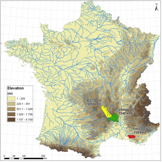
Three catchments in France, Allier (K2330810, 2269 km2), Ardèche (V5064010, 2240 km2), Arc (Y4122020, 728 km2) are selected for this study. Figure 3 shows the location of three study catchments in France. These catchments are selected because they have available data necessary for uncertainty quantification performed in this study, such as spatially averaged precipitation and ensemble discharges from rating curve are available in these areas. Besides, these catchments are part of a wider study on uncertainty quantification and propagation conducted at Cemagref. Some characteristics of the catchments are summarized in Table 1. Two catchments Allier and Ardèche, which are medium sized catchments with area of more than 2000 km2, are located in the mountainous area while Arc, the small catchment with only 728 km2, is in a lower area.
Figure 3: Location of the three study catchments with indication of their codes and surface areas
CemOA
: archive
ouverte
d'Irstea
Table 1: Study areas and data availability
2.2
Observed precipitation and discharge data
The observed precipitation is used as input for the GRP model in the calibration period. In the forecast period, observed precipitation is used to simulate the discharge until the day of issuing the forecast. Observed discharges are used to calibrate and validate the model, as well as update the state of the model at each time step during the forecast period. Observed precipitation data come from the meteorological analysis system of Météo-France (SAFRAN) and observed streamflow data come from the French database Banque HYDRO. The data used in this research is daily data.
The observation period of precipitation is from 1/8/1958 to 31/7/2009 (about 51 years). During this period, availability of discharge data varies with catchments, as shown in Table 1; catchments Allier and Ardèche have long series of discharge while catchment Arc has only about 14 years. With GRP calculation algorithm, when no data of discharge are found, the model still simulates in the days with no data but the objective functions are calculated without those days. Hence, it will not affect too much the calibration and validation if the number of missing values is small and scattered in the whole period. For catchment Arc, the data are still available for about 14 years so it is still acceptable for calibrating and validating the model. Besides, it would be also interesting to look at catchment Arc because it is a small catchment (728 km2) compared with the other two with quite similar size (2269 km2 and 2240 km2). CemOA : archive ouverte d'Irstea / Cemagref
2.3
Forecasting system and GRP model
2.3.1
Forecasting system
A forecasting system contains many different components as shown in Figure 1. Forecasting ensemble river discharge with a hydrological model requires defining a particular model structure, with its parameters, input data and, usually, an updating procedure to start the forecasts from initial conditions as close as possible to observed conditions. This composes a forecasting model.
To implement a hydrological forecasting model, it is thus necessary to provide the input meteorological data (precipitation, temperature, etc.) for flow simulation and weather forecast (precipitation, temperature, etc.) to predict the river flow. The initial state of the system needs also to be defined so that the forecast can start from a certain, properly defined point. This initial state can be defined without a specific updating routine based only on the simulated discharge at the end of the previous time step, which already takes into account observed meteorological conditions. However, as the model flow output contains errors due to the limited representation of the real system, the simulated discharges are also subject to some errors, which might be exacerbated in time during the continuous simulation of the hydrological model. Therefore, in order to avoid such errors, other kinds of observed data, for example observed discharges can be used to update the forecasting model and bring its output closer to real time conditions before issuing a forecast. It should be kept in mind, however, that the observed discharges are not error free, as observation is still far from being perfect due to the instrumental errors and the difficulties of capturing the natural space-time variability of stream flows. As the model represents the real system through a set of parameters that characterizes that system, the parameters need to be defined before using the model to forecast. In order to define the model parameters, the model is calibrated using a long period of historic data (called calibration period); after calibration, the model can be used for forecasting. Calibration and forecasting period need to be independent.
Finally, after issuing a forecast, the output of the model, the forecast discharge, should be compared with a reference value to evaluate the forecast performance. This reference discharge can be the observed discharge. Here again, as the observed discharge is also subject to measurement errors, using it as reference might lead to a wrong interpretation of forecast outcome.
2.3.2
GRP model structure and parameters
The hydrological model used in this research is the GRP model, integrated in the GRPE forecasting system to forecast discharges from an ensemble of forecast precipitation scenarios at each forecast time step. Weeink (2010) and Berthet et al. (2009) provided a detailed description of the model structure. Here, a summarized description is presented. More detailed information about the model can be found in the above papers.
The GRP model is a daily lumped hydrological forecasting model developed in Cemagref, France (Figure 4). CemOA : archive ouverte d'Irstea / Cemagref
Model inputs are the areal rainfall P, either observed or forecast for stream flow simulating and forecasting respectively; and the potential evapo-transpiration PE. In practice, the climatological value for the potential evapo-transpiration is used (for example, the same seasonally variable evapo-transpiration, identically repeated each year), as previous studies have shown that, for the family of GR models, there were no systematic improvements in the rainfall-runoff model efficiencies when using temporally varying evapo-transpiration (Oudin
et al., 2005). Figure 4: Model structure of the GRP hydrological forecasting model (Berthet et al., 2009)
The GRP model consists of a production function and a routing function as shown in Figure 4. The model describes the hydrologic process from rainfall to runoff as a sequence of processes in one time step. The time step used in this study is daily time step.
The GRP model consists of three calibrated parameters: the volume adjustment factor which controls the volume of effective rainfall X1; the level of the routing store X2 and the base time
of the unit hydrograph X3.
Besides, a number of fixed parameter is defined for the forecasting model running at daily time steps:
• Production reservoir capacity: A=350mm • Percolation function coefficient: B=2.25 • Unit hydrograph exponent: α=2.5
• Outflow routing reservoir exponent: β=2.0
2.3.3
Calibration, validation and forecast in the GRPE forecasting system
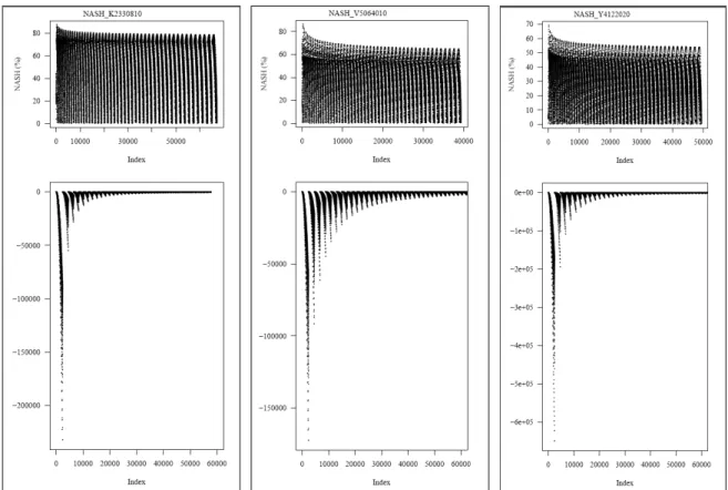
The GRP parameters are calibrated using the historic data of discharge. The calibration and validation are done automatically. Optimization searches for the global optimum of a given objective functions. Four performance criteria are automatically computed by the calibration-validation routine:
Root Mean Square Error:
ˆ 2 Q - Qt+L t+Lt t RMSE(L) =
n
[1] CemOA : archive ouverte d'Irstea / CemagrefPersistence index:
(
)
ˆ 2 Q - Qt+L t+L t t PI(L) = 1 - 2 Q - Qt t+L t .100% [2] Nash-Sutcliffe: ˆ ˆ 2 Q - Qt+L t+L t t NASH(L) = 1 -2 Q - Q t+L t t .100% [3]Transformation of Persistence Index:
PI(L) C2MP(L) = 100. PI(L)
100
2
-100
[4] where L is the lead time, Qt and Qt+L are the observed discharges at time step t and t+Lrespectively; Q is the average of observed discharges; while Qˆ
t +L t is the forecast issued at
time step t for time step t+L; n is the number of time steps.
The model uses all observed data previously to the start of forecast period to calibrate its parameters. The optimization searches to maximize the PI values. When forecasting, the model simulates stream flow until the day of issuing the forecast, and then forecast the flows for the L days after depending on the length of lead times.
CemOA
: archive
ouverte
d'Irstea
3
Methods
In this chapter, literature is reviewed to identify the possible uncertainty sources that might propagate into the forecasting system of interest; as well as to determine which sources play a crucial role in this system. Based on that, methods for quantifying each of those “important” sources of uncertainty is described together with the corresponding data that are used. After that the method for experimental uncertainty propagation is introduced. At the end, the evaluation measures for assessing the uncertainty quantification are described.
3.1
Identifying uncertainty sources
3.1.1
Initial identification of uncertainty sources
A large number of researches on uncertainty of hydrological modelling or flow forecasting can be found in the literature, for example, Uhlenbrook et al. (1999), Carpenter and Georgakakos (2004), Mc Milan et al. (2010), Kuczera et al. (2010), etc. Therefore, it is useful to make use of the existing knowledge to study possible sources of uncertainty in a system. Besides, there are also different methods for doing this work; for instance, one might use the expert opinion method proposed by Warmink et al. (2010). Whatever method is applied to identify the sources of uncertainty, literature study is definitely an inevitable step. Here this method is used for identifying the uncertainty sources that play a role in hydrological forecasting in general and GRPE flow forecasting system in particular.
In the hydrological modelling context, Walker et al. (2003) categorized five uncertainty sources (or "location" as the authors used in their papers) which are context, model, inputs, model parameter, model outcome uncertainty. The model outcome uncertainty is the result of propagating the other uncertainty sources through the model; so basically there are four sources that might cause the uncertainty in hydrological modelling.
Context is an identification of the boundaries of the system to be modelled, and thus the portions of the real world that are inside the system, the portions that are outside, and the completeness of its representation. Because it is related to the limitation of the model by which the real world cannot be fully described, here the context is classified in the uncertainty source arose from the model.
In addition, the model uncertainty has two other categories, model structure uncertainty and model technical uncertainty. The model technical uncertainty is generated by the software or hardware errors. In case of GRP model, this is a lump, conceptual model with a simple code which is written in FORTRAN language; therefore, the model is expected to be not subject to the model technical uncertainty. The model structure uncertainty arises from a lack of sufficient understanding of the system, including the behaviour of the system and the interrelationships among its elements. Model structure uncertainty also involves the mathematical algorithm, equations and assumptions of the model. In GRP model structure, the uncertainty can come from the representation of rainfall-runoff process using the production and routing reservoirs, or the definition of a threshold level according to that the
CemOA
: archive
ouverte
d'Irstea
amount of evapo-transpiration is decided, or the hydrological routing process which is described by the unit hydrograph.
The input data uncertainty is divided by Walker et al. (2003) into uncertainty about the external driving force and uncertainty about the system data. The external driving force that produces changes within the hydrological process is the meteorological force; in the case of GRP forecasting model, it is the input precipitation data used for the flow simulation mode of the system. The uncertainty about the system data including land use map, data on water-related infrastructure, which is often the result of the lack of knowledge on the system’s properties, is not applicable to the GRP model, so it is not considered in this research. Finally, it should be noted that in their paper, the authors considered the uncertainty in hydrological modelling, not forecasting; in a hydrological forecasting system, there is another uncertainty which can be also classified as uncertainty about the input data. This is the uncertainty from the forecast driving force or the forecast precipitation which is used for flow forecasting in the GRPE system.
Concerning the model parameter uncertainty, there are four different types of parameters suggested by Walker et al. (2003), divided into two sub-categories: non-calibrated parameters and calibrated parameters. Non-calibrated parameters include: (1) Exact parameters (universal constants); (2) Fixed parameters (well defined parameters like gravity acceleration g); and (3) Prior chosen parameters (which are parameters that may be difficult to identify by calibration and are chosen to be fixed to a certain value that is considered invariant). In the GRP model, as mentioned in Section 2.3.2, there are four main parameters whose values are fixed. The uncertainty of non-calibrated parameters can come from the fact that these parameters are chosen and fixed at some values. The calibrated parameters are unknown with previous experience and need to be determined by minimizing the difference between model outcomes and measured data of the same period and location. Here these are the three calibrated parameters of GRP. The choice of these parameters when forecasting river flow can affect the forecast outcome and cause uncertainties.
In Walker et al. (2003), the uncertainty coming from the initialization of the model is not mentioned. However, this source of uncertainty was investigated by other authors (for example, Berthet et al. (2009)). For the GRP model, at each forecast day, the state of the system is updated with the observed discharge at the end of the previous time step. However, this choice of initial condition might also lead to uncertainties in the discharge forecasts as the observed discharge might contain errors and might not be a good start for the simulation at the forecast time step. Another uncertainty source which is also not mentioned in Walker et al. (2003) but was studied in the literature is uncertainty of the observed discharge (See Mc Milan et al. (2010)). As the outcome of the forecasting model is compared with the observed discharges, which is an uncertain reference, this action might cause a misinterpretation of the results if the uncertainties are not considered.
The uncertainty in hydrological forecasting is the accumulated uncertainty of the above uncertainties. All sources of uncertainty in hydrological forecasting are summarized Figure 5 below: CemOA : archive ouverte d'Irstea / Cemagref
Figure 5: Different uncertainty sources that can propagate into hydrological forecasting
In the context of GRPE forecasting system, the uncertainty sources are shown in Figure 6.
Figure 6: Identification of uncertainty sources for GRPE forecasting system
CemOA
: archive
ouverte
d'Irstea
3.1.2
Determination of uncertainty source importance
As discussed above, there are different sources of uncertainty in hydrological modelling and forecasting; and the literature shows that those uncertainties do not have the same influence on the outcome flows; some might have very large influence and others might have
impact. For example, the uncertainty about the non-calibrated parameters is not mentioned in the literature as an important source of uncertainty that should be considered in uncertainty propagation. In this step, previous researches are considered to determine the most important uncertainty sources to set the focus for uncertainty quantification and propagation in the next steps.
Among all of those uncertainties, meteorological input uncertainty is usually assumed to be the largest source of uncertainty in the prediction of floods, at least for lead times of 2-3 days (Rossa et al., 2010). He et al. (2009) also showed that forecast precipitation uncertainties dominate and propagate through the cascade chain. The input uncertainty is significant because of the high spatial and temporal variability of precipitation (Kavetski et al., 2006). Hence, attention should be paid on this sort of uncertainty when assessing the flood forecast uncertainty.
The initial moisture conditions at the beginning of a rainfall event have a major influence on a catchment’s hydrological response and therefore have a crucial impact on flood forecasting. Berthet et al. (2009) analyzed the influence of initialization on flood forecasting for 178 catchments in France. They found that different methods of initialization could result in very large differences in the flood forecasts. A persistence index was used to evaluate the discharge forecasts; and the result of their research shows that at the 1-hour lead time, the persistence differences for different (arbitrary) initial values are greater than 0.03 (which is a significant difference) on more than 75% of the catchments; for the 48-h lead time, this difference is greater than 0.14 for more than 90% of the catchments. Schaake et al. (2006) also emphasized that one of the most important source of hydrological model uncertainty is the uncertainty in initial conditions.
Beside the uncertainty caused by the selection of initial condition, the model structure and parameterization uncertainties are also significantly pronounced in flow forecasting. A study done by Butt et al. (2009) shows that the sensitivity of streamflow simulations to variations in acceptable model structure was at least as large as uncertainties arising from parameter and observation uncertainty. The authors stated that model performance was strongly dependent on model structure.
Hughes et al. (2010) also reported on relatively large uncertainties of the hydrological model they used related to parameter values even when the input data uncertainty was not taken into account. Authors suggested that the forecast uncertainty will be probably larger when the input uncertainty is considered.
The examples in their research suggest that there are differences in the degree of parameter value uncertainty for sub-basins that have different physiographic, climate and runoff response characteristics. CemOA : archive ouverte d'Irstea / Cemagref
Uhlenbrook et al. (1999) studied the prediction uncertainty of conceptual rainfall-runoff models caused by problems in identifying model parameters and structure. The authors also reported the importance of accounting for model structure and parameter uncertainty when evaluating the forecasting uncertainty. They noted that the difficult identifiability of the model structure caused uncertainties in the flow predictions but they were slightly smaller than the implications caused by the parameter uncertainty. However, perhaps this conclusion comes from the rather similar HBV model variants tested in this study. The variations of simulation results would probably increase for predictions with totally different conceptual rainfall-runoff models.
Mc Milan et al. (2010) studied the errors in discharge measurements used to calibrate a rainfall runoff model, caused by the rating curve uncertainty. The authors recognized that serious considerations of uncertainties in discharge data can significantly improve the prediction ability of the model. This implies the importance of accounting for observed discharge data uncertainty in flow forecasting.
In summary, there are some uncertainty sources, which are found important in flow simulating and forecasting in the literature, namely uncertainty about the input data (external driving forces, forecasting driving force), initial conditions, model parameters, and model structure.
To be more specific to the case of the GRPE forecasting system used in this study, hereafter, the uncertainty of external driving forces is referred to as input precipitation uncertainty; and the uncertainty of forecast driving force is referred to as forecast precipitation uncertainty. These important uncertainty sources are listed in Table 2.
Table 2: Main sources of uncertainty in flood forecasting
Sources of uncertainty Importance References
Input data uncertainty
Uncertainty about input precipitation High Rossa et al. (2010) Uncertainty about the forecast
precipitation
High He et al. (2009)
Uncertainty about the system data Low
Model uncertainty
Context Low
Model structure uncertainty High Butt et al. (2009)
Uhlenbrook et al. (1999)
Model technical uncertainty High
Model parameter
Uncertainty about non-calibrated parameters
Low Uncertainty about calibrated
parameters
high Butt et al. (2009)
Hughes et al. (2010)
Initial conditions Uncertainty about the current state of
the system
high Berthet et al. (2009)
Observed discharge Uncertainty from the rating curve High Mc Milan et al. (2010)
CemOA
: archive
ouverte
d'Irstea
3.2
Quantifying the impact of individual uncertainty on flood forecast
In this research, there are five main sources of uncertainty are investigated, namely (1) input precipitation uncertainty, (2) forecast precipitation uncertainty, (3) initial condition uncertainty, (4) calibration period uncertainty, (5) parameterization uncertainty. The uncertainty about the model structure is not considered here due to time constrain as it would require using several other model structures, but could be another source of uncertainty to be considered for future research. The materials those are used to account for the uncertainties are described below; the individual uncertainty tests are explained at the end of this section.
3.2.1
Input precipitation uncertainty
The observed rainfall data that are often used for catchment studies are often not areal rainfall because rainfall cannot be quantitatively measured in space with sufficient precision for catchment modelling. Usually, rainfall is only observed at some stations (point rainfall), located either inside or outside the study catchment. In order to simulate rainfall-runoff process in the whole basin area, it is necessary to spatially interpolate point data. There are many methods used for interpolating and averaging rainfall, as, for example, the Thiessen polygon method, the arithmetic mean method, the isohyetal method (Shaw, 1994). It is a fact that none of these methods can properly produce an areal rainfall; and the uncertainty from the methods combined with uncertainties from the instruments used to measure precipitation, leads to errors in observed rainfall data used in hydrological modelling.
In this research, to account for the uncertainty of observed rainfall, precisely the uncertainty of transforming point rainfall to areal rainfall (errors from rain gauge instruments are neglected), the areal rainfall generator developed at Cemagref is used. This generator is based on the geo-statistical Turning-Bands-Method (TBM) for the simulation of random field and has been applied for characterisation of rainfall intensities (Ramos, et al., 2006). The version used in this research comes from recent developments made at Cemagref (Lepioufle, 2009). It first applies the conditional simulation method to hourly rainfall observed data and then aggregates the different simulated fields to daily time steps. Conditional simulation is a geo-statistical method that generates multiple geo-statistical realizations of the spatial rainfall field over a specific area, while preserving the information measured by the individual rain gauges. Spatial and temporal structures are also preserved in the simulations. The rainfall generator is built from the analysis of variograms and the evolution of spatial structure with time. Besides, rainfall fields are generated according to different successive rain types, defined by using a Kohonen algorithm and statistical properties of non-zero precipitation and total coverage area.
For this research, the rainfall generator is set up for one of the study catchments, catchment Ardèche. We then ran the simulator for the period from 2000 to 2008. Ten realisations (members) are generated at each hourly time step. Figure 7 Illustrates 4 generated fields of spatially distributed rainfall over catchment Ardèche for the day 12/01/2004 at 13:00.
CemOA
: archive
ouverte
d'Irstea
Figure 7: Four out of ten simulations of spatially distributed rainfall over catchment Ardèche on 12/01/2004 at 13:00. Rain gauges are presented by squares. Each realisation preserves the observed data at the rain gauges
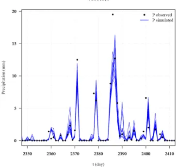
Figure 8: Ten simulated areal precipitation values for catchment Ardèche from 07/06/2006 to 06/08/2006 (blue lines). Observed precipitation given by the SAFRAN Météo-France data analysis system is also indicated (black dots). CemOA : archive ouverte d'Irstea / Cemagref
From the geo-statistical conditional simulation, every simulation is a possible realization of the rainfall over the catchment. Because the hydrological model applied in this research is a lumped model running at daily time steps, the distributed hourly rainfall fields were aggregated in space (average precipitation over the catchment area) and in time at daily time steps. As a result, 10 values of areal rainfall are available at each day of the forecast period. They represent observed rainfall uncertainty at the catchment scale, as illustrated on Figure 8, 10 series of spatial averaged rainfall are plotted in a period of 2 months together with the observed rainfall data from SAFRAN. These members of spatially averaged rainfall are used as input rainfall for the GRP model to assess the impact of input data (observed precipitation) uncertainty.
3.2.2
Forecast precipitation uncertainty
The weather observation is no way perfect or complete because of the chaotic atmosphere system which causes the difficulties in predicting. In addition, because of the limitation in numerical computer modelling, the weather system is inevitably an approximation of the exact solutions of the equations describing the system. Therefore, every weather forecast contains, to some extent, uncertainty. This uncertainty is unfortunately not constant but varies from day to day, depending on the stability of the atmospheric condition at the start of the forecast. The major uncertainty of weather forecasts comes from the estimation of the initial state of the atmosphere and from unavoidable simplifications in the representation of the complex nature in weather numerical models (European Centre for Medium-Range Weather Forecasts, 2011). For that reason, deterministic forecasts, which produce only one forecast based on the best estimate of the future event, are no longer suitable for many applications in practice, as uncertainty is not attached to the forecasts.
In order to deal with the problem of the weather forecast uncertainty, Ensemble Prediction Systems (EPS) were developed by several meteorological forecast centres. It is a kind of probabilistic forecast that represents the uncertainty in both initial conditions of the atmosphere and the numerical model used. Instead of using only one best estimate of the initial condition, slightly different states of the atmosphere, which are close but not identical to the best estimate, are used. Additionally, each forecast is based on a model (or on a different parameterization of a model), which is close but not identical, to the best estimate model equations. The result is not only one, but a number of forecasts spreading around the “control member”, which is based on the best estimate of initial state. This technique provides an estimate of the uncertainty associated with predictions from a given set of initial conditions compatible with observation errors. If the atmosphere is in a predictable state, the spread will remain small; if the atmosphere is less predictable, the spread will be larger. In a reliable ensemble prediction system, reality will fall somewhere in the predicted range. This means that users get information on the actual predictability of the atmosphere, for example, whether a particular forecast can be expected to be certain or less certain. In addition, they also get information on the range within which they can expect reality to fall.
In this research, two EPS products are used, one from the European Centre for Medium-Range Weather Forecasts (ECMWF) and the other from the forecast ensemble system
CemOA
: archive
ouverte
d'Irstea
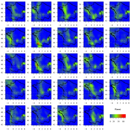
developed at Météo-France (PEARP). An example of an ECMWF EPS forecast over France is given in Figure 9.
Figure 9: Maps of 24 (out of 51) members of EPS forecasts from ECMWF in France on 24 May 2008 at lead time of 4 days
ECMWF EPS data are archived forecasts and consist of one control member and 50 perturbed members, making a total of 51 forecasts at each day of the forecast period. The system focuses on medium-range forecasts (from 3 days onwards). Data was provided at a spatial resolution of 0.5° x 0.5° latitude-longitude (equivalent to spatial grid of approximately 50 km in France) and at variable time step, up to a lead time of 14 days. For this study, areal forecast precipitation was available for each catchment at daily time steps for the period from 11/03/2005 to 30/09/2008.
The Météo-France PEARP is focused on short-term forecast (less than 3-4 days of lead time) (Nicolau, 2002), and its application to hydrology has been recently reported in the literature (Thirel et al., 2008; Randrianasolo et al., 2010). Data for this study is available at spatial grid of 8 x 8 km over France and 3-hourly time steps. The number of members is limited to 11 members including one control member, and the maximum lead time is two days. For this
CemOA
: archive
ouverte
d'Irstea
study, areal forecast precipitation data are available for each catchment at daily time steps for the period from 11/03/2005 to 31/07/2009.
Because of its higher resolution, PEARP is used for the 1- and 2- day forecast lead times, while ECMWF EPS is used for lead times from 3 to 9 days. The predictions from ECMWF EPS for longer lead times are not used because after 9 days the resolution reduces, as well as the skill of the forecasts.
3.2.3
Initial condition uncertainty
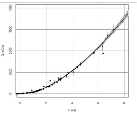
The discharge data that are often used in hydrologic studies are not direct observed flows but they are usually retrieved from the rating curve – a relation curve between discharge and water level. Normally, the rating curve is constructed with a series of historic measured river flows and water levels. After that, water levels are measured continuously and, based on the value on the rating curve, discharge values are estimated. The values of discharge are regularly checked with the measurement but not for every time. Details about discharge measurement and rating curve construction can be reached at Shaw (1994).
Discharge data are subject to three kinds of errors: errors from discharge measurement, errors from rating curve fitting, and errors from water level measurement.
The errors in the discharge measurements can come from the operational condition during gauging or from insufficient number of verticals, from insufficient number of point velocity measurements per vertical or from the flow variation during the measurement period, etc. The rating curve fitting error is caused by the imperfection of the relationship curve, even if the true water stage and discharge were known. Water levels are usually assumed to be error free, although errors associated to the measurements device can exist. Therefore, uncertainty always exists when the rating curve is used to estimate the flow values.
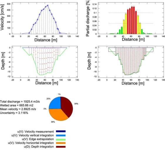
In this research, initial condition uncertainty is assessed through the rating curve uncertainty, which is estimated for each catchment using a Bayesian approach (Renard et al., 2011). In the first step, the uncertainty in each individual gauging is quantified. It depends on the gauging method (e.g. velocity-area method, tracer dilution, ADCP, surface velocity measurements, etc.) and the operational characteristics of the gauging (e.g. spatial sampling of velocity and depth throughout the cross-section, unsteadiness of the flow, etc.). A set of standard deviations representing the measurement uncertainty affecting each gauge is withdrawn after this step. The output is illustrated on Figure 10.
CemOA
: archive
ouverte
d'Irstea