HAL Id: hal-01622564
https://hal.inria.fr/hal-01622564v2
Submitted on 27 Nov 2017
HAL is a multi-disciplinary open access
archive for the deposit and dissemination of
sci-entific research documents, whether they are
pub-lished or not. The documents may come from
teaching and research institutions in France or
abroad, or from public or private research centers.
L’archive ouverte pluridisciplinaire HAL, est
destinée au dépôt et à la diffusion de documents
scientifiques de niveau recherche, publiés ou non,
émanant des établissements d’enseignement et de
recherche français ou étrangers, des laboratoires
publics ou privés.
Grouping Answers in Ontology-Based Query Answering
Maxime Buron
To cite this version:
Maxime Buron. Grouping Answers in Ontology-Based Query Answering. Logic in Computer Science
[cs.LO]. 2017. �hal-01622564v2�
Grouping Answers in Ontology-Based Query Answering
Maxime Buron
Supervised by Michaël ThomazoNovember 27, 2017
Contents
1 Introduction 1
1.1 Context and Motivation . . . 1
2 Recall of OBQA Problem & Approches 2 2.1 Basic Logical Notations . . . 3
2.2 Ontology-Based Query Answering Problem . . . 3
2.3 Rewriting Approach with Existential Rules . . . 4
3 Problem Statement 5 4 Rewritings Graphs 6 4.1 Definition & Properties . . . 6
4.1.1 Definition of the Rewriting Graph . . . 6
4.1.2 Construction of the Rewriting Graph . . . 7
4.2 RDFS rewriting . . . 10
4.3 Product of Graph . . . 10
5 Labellisation 12 6 Implementation & Experiment 15 6.1 Resources . . . 15
6.1.1 Datasets . . . 15
6.1.2 Implementation . . . 16
6.2 Computation of the Rewriting Graph . . . 16
6.3 Building Labellisations . . . 16
7 Future Work 17
Abstract
We aim at easing the use of semantic and structured data by improving the restitution of answers. Instead of providing a set/ ranked list of answers, we devise techniques to group answers and to semantically label the group in an informative way, easing further exploration of the answers.
1
Introduction
1.1
Context and Motivation
Among the wealth of resources that are currently available on the Internet, there exist some that have very interesting features for an automatized processing: those that are both structured and endowed with a semantics. Structured data allows for formal querying, whose precision is much higher than that of an intuitive but rather vague keyword querying. Semantics ease the formulation of queries, allowing the user to use a vocabulary with which he/she may be familiar with, ignoring the implementation details.
Such semantic and structured data has been widely made available, often under open licenses. Some of the flagship so-called knowledge base include DBPedia [LIJ+15], Wikidata [VK14] or YAGO [MBS15]. While the potential use cases of such knowledge bases are far reaching, their exploitation is still only starting. We believe that such is the case for several reasons, two of which we shortly elaborate on. First, writing queries in a structured query language, allowing to fully exploit the potential of structured data,
is a task that requires some training. Second, while semantic querying may theoretically provide more complete answers, this is hardly the case with current knowledge base, as it is still usually faster to fulfill an information need with classical keyword search on well-known web search engines than through a SPARQL query. The payoff for learning to write structured queries is thus too small to motivate a large number of users to spend the time learning a new way to query knowledge bases.
In this paper, we propose a novel way to exploit structured and semantic querying, providing an added value that is not only completeness of the results, but also an enhanced restitution of them. To illustrate our contribution, let us consider the case of a user willing to know more about sport leagues around the world. A first approach would be to make a keyword query on a web search engine. Current engines typically refer to Wikipedia pages, providing a list of sport leagues, manually curated. An alternative approach would be to issue a query on a knowledge base, say DBPedia. Such a query would get an unordered list of more than 3000 results. This already provides more data than the similar keyword search, but more answers alone does not mean that it fulfills in a better way the information need of the user: a few thousands answers is already too much to be efficiently grasped by a human user.
To alleviate this problem, several methods have been introduced. First, a list of answers may be returned not in a random order, but in an order that may reflect the user interest, and potentially only return the top-k answers [IBS08]. This assumes however a prior knowledge (or estimation) or the user interest, and hides (in practice) a very large part of the results. Another method is based on clustering method [DHS00]: using some features, answers are clustered and an element of each cluster is returned to the user. A shortcoming of such methods is that clusters built in such way are not easily described in a human understandable way, making the identification of interesting subparts of the result harder.
In this paper, we propose novel methods to organize the set of answers in such a way that the user get a full overview of the result set, while having sufficiently few results to consider not to be overwhelmed. In the case of sport leagues, we may decide to group the answers by region of the world, by sport, by average revenue of players within the sports leagues, or by any other criterion that the knowledge base and/or the query may allow us to use.
Figure 1: Answers of the query to sports leagues group by type of sport.
In the remaining of this paper, we first recall the necessary background about semantic and structured querying (Section 2), formally state the problem (Section 3), introduce the notion of a rewriting graph which is at the core of our approach and of its own interest (Section 4), define a novel notion of labellisation (Section 5), and experimentally evaluate our approach (Section 6). We conclude by presenting possible future work.
2
Recall of OBQA Problem & Approches
We assume the reader to be familiar with first-order logic, and recall some basic notions that will be used to describe queries and knowledge, re-using the notations from [MT14]. The interested reader can consult [vHLP07].
2.1
Basic Logical Notations
We consider a vocabulary as a pair V = (P, C ), where C is a (possibly infinite) set of constants and P is a finite set of predicates. Each predicate has an arity, which is a natural integer. Unary predicates (with arity of 1) are named classes and binary predicates (with arity of 2) are named properties. A term on V is either a constant of C or a variable. An atom on V is of form p(t1, t2, . . . , tk) where p is a predicate of P of arity k and each ti is a term.
We consider the restriction of first-order logic F OL(∧, ∃), which contains exactly the formulas built with atoms, the "and" connector ∧ and the existential quantifier ∃. We denote the set of variables of a formula F by vars(F ). In a formula, a variable which is not in the scope of a quantifier is called a free variable. A formula is closed if it has no free variable.
Example 2.1. We consider two properties p and r, a class A and a constant c. With this vocabulary, we can build the following formula:
F = ∃y∃z, p(x, y) ∧ r(c, z) ∧ A(z). The variable x is the free variable of the formula F .
In the following lines, we will just consider closed formulas. So without loss of generality, we can take all formulas of F OL(∧, ∃) in prenex form (all quantifier ∃ are at the beginning of the formula) and consider it as a set of atoms. Our approach heavily rely on the notion of homomorphism.
Definition 2.2. Given two closed formulas F and G considered as sets of atoms, a homomorphism h from F to G is a substitution from the variables of F to terms of G (and which acts as identity on constants of F ) such as for all atoms p(t1, t2, . . . , tn) ∈ F, it holds that p(h(t1), h(t2), . . . , h(tn)) ∈ G; in others words h(F ) ⊂ G.
Example 2.3. If we consider the two closed formulas F = {p(x1, y1), r(y1, z1), A(z1)} and G = {p(x2, y2), r(y2, x2), A(x2)}, the substitution h = {x1 7→ x2, y1 7→ y2, z1 7→ x2} is a homomorphism from F to G.
An important notion in logic is the notion of entailment, which is classicaly denoted by the symbol |=. The following results states the link between entailment in F OL(∧, ∃) and homomorphisms.
Theorem 2.4 ([BLMS11]). Let F and G two formulas of F OL(∧, ∃). It holds that F |= G if and only if there exists a homomorphism from G to F .
2.2
Ontology-Based Query Answering Problem
We call fact a closed conjunction of atoms. A conjunctive query is a formula of F OL(∧, ∃), in case the formula is closed, we called it Boolean conjunctive query. Free variables of the query are called the answer variables.
Example 2.5. If we consider the classes P rofessor, T eacher and Reviewer, the property reviews and the constant alice, we can define the following fact D and queries q1 and q2:
• D = P rofessor(alice) ∧ Reviewer(alice) • q1= ∃v∃wT eacher(v) ∧ reviews(v, w) • q2(x) = P rof essor(x)
q1 is a Boolean conjunctive query and q2 conjunctive query, which has a single answer variable x. Given a fact D, an answer to a query q with free variables {x1, x2, . . . , xn} is the restriction to {x1, x2, . . . , xn}of a homomorphism h from q to D. In particular, we have D |= h(q).
The behavior in this example is not fully satisfying, as it does not take the additional knowledge that we have on professors and teachers into account: indeed, we know that all professors are actually teachers. We tackle this by introducing existential rules [BLMS11], which are a formalism to represent formal definitions of domain knowledge, also known ontologies. Note that we could have alternatively used Description Logics [BCM+03].
Definition 2.6(Existential Rule). An existential rule R is a first-order formula with the following form: R = ∀x∀y B[x, y] → ∃zH[y, z]
where x, y, z are sets of variables and B, H are conjunctions of atoms whose variables belong to respectively x ∪ yand y ∪ z. We call B the body of the rule R, denoted body(R), H the head of R, denoted head(R). The frontier of R, denoted fr(R), is the set of variables y and z are call the existential variables of R.
Example 2.7 (Existential Rules). Using the same vocabulary as in Example 2.5, we can define the following existential rules:
• R1= ∀x Reviewer(x) ⇒ ∃y reviews(x, y), • R2= ∀x P rof essor(x) ⇒ T eacher(x).
R1 says that each reviewer reviews something. R2 says that each professor is also a teacher. We notice that in rule R1 there are no existential variables.
We call a set of rules R an ontology. A pair (D, R), where D is a fact and R is an ontology, is called a knowledge base, also denoted by K . Ontology-based query answering is the problem of finding the answers of a query on a knowledge base. Given a knowledge base and a (Boolean) query, an important reasoning task is to determine whether the query is entailed by the knowledge base. Several methods have been designed to this purpose. To ease the understanding, we first introduce saturation, which intuitively adds atoms that are entailed by the knowledge base to the data. We focus in the next section on an alternative approach called query rewriting, which is at the core of our approach.
Definition 2.8 (Rule Application). A rule R is applicable to a fact D if there exists a homomorphism h from the body of R to D. The result of the application of R with respect to h is π(D, R, hsaf e) = F ∪ hsaf e(head(R)), where hsaf e is a substitution on variables of head(R) that replaces a variable x by h(x)if x ∈ fr(R) and by a fresh variable otherwise.
One can apply a rule on a fact that results from a rule application, hence leading to the notion of derivation sequence.
Definition 2.9 (Derivation Sequence). Let K = (D, R) be a knowledge base. An R -derivation se-quence of D is a finite sese-quence (D0 = D), D1, . . . , Dn such as for 0 ≤ i ≤ n, there is Ri ∈ R and a homomorphism hi from body(Ri) to Di such as Fi+1= π(Di, Ri, hi).
Example 2.10. We can apply the rule R1 = ∀x Reviewer(x) ⇒ ∃y reviews(x, y) to D = P rof essor(alice) ∧ Reviewer(alice) and get the fact D1 = P rof essor(alice) ∧ Reviewer(alice) ∧ ∃x reviews(alice, x). We can apply the rule R2= ∀x P rof essor(x) ⇒ T eacher(x)to D1 and we get the fact D2= P rof essor(alice)∧Reviewer(alice)∧∃x reviews(alice, x)∧T eacher(alice). Let R = {R1, R2}, the sequence D, D1, D2 is an R-derivation sequence of D. We notice that D2 satifies q2, when D does not.
The following result states that entailment can be characterized through derivation sequences. Theorem 2.11 ([BLMS11]). Let K = (D, R) be a knowledge base and q a Boolean conjunctive query, we know that K |= q if and only if there exists an R -derivation (D0= D), D1, . . . , Dk such that Dk|= q.
2.3
Rewriting Approach with Existential Rules
While saturation is a very intuitive approach to OBQA, an alternative approach that we will exploit in our approach is the so-called query rewriting approach. Instead of modifying the data in such a way that queries can be evaluated directly over the modified data, the query is modified in such a way that the modified query can be evaluated directly over the original data. We need a few technical tools to define this approach. For the ease of understanding, we only present the rewriting method on Boolean conjunctive queries, but it can be generalised for conjunctive queries.
Definition 2.12 (Separating Variables). Let q be a Boolean conjunctive query and be q0 a subset of q, the set of separating variables of q0 is denoted by sepq(q0)and is defined as:
sepq(q0) = vars(q \ q0) ∩ vars(q0)
Definition 2.13 (Piece Unifier). Let q be a Boolean conjunctive query and R be an existential rule. A piece unifier µ = (q0, u) of q with R is such as q0 ⊂ q and u is a function from vars(q0) ∪ fr(R) to const(q0) ∪ terms(head(R))such as:
• for all y ∈ fr(R), u(y) ∈ fr(R) or u(y) is a constant; • for all x ∈ sepq(q0), u(x) ∈ fr(R) or u(x) is a constant; • u(q0) ⊂ u(head(R)).
Definition 2.14 (Direct Rewriting). Given q a Boolean conjunctive query, R an existential rule and a piece unifier µ = (q0, u)of q with R, the direct rewriting of q with µ, denoted β(q, R, µ) is u(body(R) ∪ (q \ q0)).
Example 2.15 (Direct Rewriting). If we use the notation from Example 2.5 and 2.7, we can find two direct rewritings of q1 by applying either R1 or R2. Considering R1, we find the following piece unifier µ1 = (q1, u1) where q10 = {T eacher(v)}, u1 = {v 7→ x} and the direct rewriting of q1 with µ is q3 = ∃x∃w P rof essor(x) ∧ reviews(x, w). Considering R2 on q3, we find the following piece unifier µ2 = (q03, u2), where q03 = {reviews(x, w)}, this time the separing variables is not the empty set, but contains x. The direct rewriting of q3 by µ2 is the query q4 = ∃x∃y, P rof essor(x) ∧ Reviewer(x). We notice that D entails q4 from the Example 2.5 – hence this is an example of how rewriting the query enables to find more results than the original query.
As in the saturation case, it is possible to apply a rewriting step on a query that has been generated by a first rewriting step. This leads to the notion of rewriting sequence.
Definition 2.16 (Rewriting Sequence). A sequence of queries q0, q1, . . . , qk is a R-rewriting sequence of q0 if for each 1 ≤ i ≤ k, it exists a rule Ri ∈ R and a piece of unifier µi of qi−1 with R such as qi= β(qi−1, Ri, µi).
Definition 2.17 (R-rewriting). Let q be a Boolean conjunctive query and R be a set of existential rules, qk is a R-rewriting of q if there exists q0= q, q1, . . . , qk a R-rewriting sequence of q.
We recall the following theorem, proving that the above notion of query rewriting is adequate. Theorem 2.18([BLMS11]). Let D be a fact, R a set of existential rules and q be a Boolean conjunctive query, D, R |= q if and only if there exists q0 a R-rewriting of q such that D |= q0.
In our approach, we will often exploit the following corollary of Theorem 2.18.
Corollary 2.19. Let q be a Boolean conjunctive query, R a set of existential rules and q0 a R-rewriting of q, then q0, R |= q.
Proof. We knows that q0 is a R-rewriting of q such as q0 |= q0, using Theorem 2.18 and since q0 can be seen as a fact, we know that q0, R |= q.
Let us notice that the set of rewritings of a query with respect to a set of rules R is not necessarily finite, as witnessed by the following example.
Example 2.20. Let us consider the query q = r(a, b) and the rule ∀x ∀y r(x, y) ∧ r(y, z) → r(x, z). Any query of the shape r(a, x1) ∧ r(x1, x2) ∧ . . . ∧ r(xn, b), for any n, is a rewriting of q. There exists thus an infinity of (non-equivalent) R-rewriting of q.
Of special interest to our approach are sets of rules whose set of rewritings admits a finite covering. In other words, there exists a finite set of query Q such that for any fact D, it holds that D, R |= q if and only if there exists q0 ∈ Q such that D |= q0. Sets of rules ensuring that there exists such Q are called finite unification sets [BLMS11], and prominent exemple of such sets of rules are aGRD, linear [CGK13] or sticky rules [CGP10].
3
Problem Statement
Given a query q and a knowledge base (D, R), we want to find interesting semantically defined subsets of the answers of q. We formalize this through the notion of labellisation of a query. For the sake of generality, we define this notion for first-order queries and not only formulas of F OL(∧, ∃).
Definition 3.1. A labellisation L of a query q with respect to a set of rules R is a set of queries such as each q0 ∈L semantically implies q, formally:
q0, R |= q
We expect that a labellisation of a query has at least two properties: covering and simplicity. Covering states that any answer of the original query is an answer of some query of the labellisation. Simplicity states that the labellisation does not contain redundant queries.
Definition 3.2 (Covering). A labellisation L of a query q with respect to a set of rules R is called covering if :
q, R |= _ q0∈L
Definition 3.3 (Simplicity). A labellisation L of a query q with respect to a set of rules R is called simple if :
∀q1, q2∈L , q1, R 6|= q2.
Let us notice that this notion of labellisation defines a set acceptable objects. However, there exists trivial labellisations, such as {q}. Our goal is to find more interesting ones – and we will especially consider the cardinality of answers of the queries appearing in the labellisation.
4
Rewritings Graphs
As we will from now on exclusively consider conjunctive queries, we simplify the terminology and use the term “query” for conjunctive queries. We introduce the notion of a rewriting graph, which is at the core of the method presented in the next section, which returns a labellisation. The main idea behind the rewriting graph is to have a graph such as its vertices are the rewritings of the original query q and the edges contain semantic structure (entailment) relations between rewriting queries. We choose to find a labellisation in the set of rewriting queries of q, because they naturally are more precise queries than q by Proposition 2.19. We also use the way rewriting queries are build using rules which provide their semantic structure. The first Subsection 4.1 defines the general notion of the rewriting graph for existential rules. After a quick recall of RDFS and of a simpler rewriting procedure for that ontology language, Subsection 4.3 defines product graphs which can be viewed as an approximation of the rewriting graph for RDFS rules.
4.1
Definition & Properties
In this part, we define a graph of rewritings of the initial query q which contains in its edges information about entailments which exist between rewritings. In the first part, we define theoretically this graph and some of this properties. We then define the same graph using a more constructive approach. 4.1.1 Definition of the Rewriting Graph
In order to get a semantic definition of subset of answers, we define the set of all the rewritings of a query. Notation 1. Let q be a query and R a set of existential rules, we denote the set of R-rewritings of q by Nq,R. Whenever there is no ambiguity, we will abusively simplify this notation in Nq.
As it is convenient to abstract away from the syntax of rewritings, we will consider classes of queries up to semantic equivalence, as formalized in the next definition.
Definition 4.1(Class of Semantic Equivalence). Let R be a set of existential rules and S a set of q, the set of classes of semantic equivalence of S with is:
{˜qR,S/q ∈ S}, where ˜qR,S = {q0 ∈ S/q0, R |= qand q0, R |= q}.
Whenever there is no ambiguity, we will denote ˜qR,S by ˜q. We define a graph that contains all rewritings of a query with the respect of a set of existential rules and also all implication links between rewritings.
Definition 4.2 (Saturated Graph). The saturated graph of R-rewriting classes of q is the graph Gq = (V, E)defined by:
• V is the set of classes of semantic equivalence of Nq;
• E is the set of edges ( ˜q1, ˜q2) such as ˜q1 6= ˜q2 and the class ˜q2 semantically implies the class ˜q1, which means there exists q1∈ ˜q1 and q2∈ ˜q2 such as q2, R |= q1.
Proposition 4.3. Let q be a query and R be a set of existential rules, the saturated graph G of R-rewriting classes of q is an acyclic graph.
Proof. Suppose there is a cycle ˜q0, ˜q2, . . . , ˜qk in G, we know that for 1 ≤ i ≤ k, qi−1, R |= qiand ˜q0= ˜qk, So finally for 1 ≤ i, j ≤ k, ˜qi= ˜qj and there is not cycle.
Let us notice that the saturated graph of R-rewriting classes of q may be infinite, but is finite whenever Ris a finite unification set. In the remaining of this paper, we assume R to be a finite unification set. We can now define the rewriting graph of a query q, which is the version of the graph we use to extract from a labellisation. Note that this notion is well-defined, as the transitive reduction of an acyclic graph is uniquely defined. We define also this graph as a transitive reduction, because we want that all oriented paths in this graph are as detailed as possible. In other words, by definition of the transitive reduction, if we have the path ˜q0, ˜q1, . . . , ˜qk in the rewriting graph, we know that for all 1 ≤ i ≤ k, there is no rewriting q0
i of q such as q0i∈ ˜/qi−1∩ ˜qi and such as qi−1, R |= q0i and q0i, R |= qi.
Definition 4.4 (Rewriting Graph). The rewriting graph of a query q with respect to a set of existential rules R is the transitive reduction of the saturated graph of R-rewriting classes of q.
4.1.2 Construction of the Rewriting Graph
In this subsection, we prove that Algorithm 1 builds the rewriting graph of a query q with respect to a set of existential rules R. Algorithm 1 works as follows: Lines 4 to 14, the graph of rewriting process is built. Lines 15 to 18, all homomorphisms links are added to the edges of the graph. Strongly connected components are then merged (Line 21, by MergeStronglyConnectedComponents(G)) and the transitive reduction is computed by TransitiveReduction(G) and output. We do not provide more details about the done by TransitiveReduction and MergeStronglyConnectedComponents, as these operations are rather classical.
Input: A conjunctive query q, a finite unification set R Output: The rewriting graph of q w.r.t. R
1 V = {q} 2 E = ∅ 3 N = {q}
4 while N 6= ∅ do 5 Pick q0 ∈ N
6 forany direct R-rewriting q00 of q0 do 7 if there is no ˆq ∈ V s.t. ˆq |= q00 then 8 V = V ∪ {q00} 9 E = E ∪ {(q0, q00)} 10 N = N ∪ {q00} 11 end 12 end 13 N = N \ {q0} 14 end 15 for (q, q0) ∈ V × V do 16 if q |= q0 then 17 E = E ∪ {(q0, q)} 18 end 19 end 20 G = (V, E) 21 G = MergeStronglyConnectedComponents(G) 22 G = TransitiveReduction(G) 23 returnG Algorithm 1: ComputeRewritingGraph(q, R)
First we use the process of rewriting to build a graph of queries that contains the rewritings of a initial query.
Definition 4.5 (Graph of Rewriting Process). The graph of rewriting process of a query q with respect to a set of existential rules R is the graph G = (V, E) where V = ∪+∞
k=1Vk and E = ∪+∞k=1Ek such as V1= {q}, E1 = {} and for strict positive integer k sets Vk+1 and Ek+1 are defined by(the function β is defined in Definition 2.14):
• Vk+1= Vk∪ {β(q1, R, µ)|∃q1∈ Vk, ∃R ∈ R, µis a piece of unifier of q1 with R}, • Ek+1= Ek∪ {(q1, β(q1, R, µ))|∃q1∈ Vk, ∃R ∈ R, µ is a piece of unifier of q1 with R}.
Proposition 4.6. The vertices of the graph of rewriting process of a query q with respect to a set of existential rules R is the set of rewriting of q with the respect of R.
Proof. We prove by induction that for all strict positive integer k the graph Gk = (Vk, Ek)where Vk and Ek are defined as in Definition 4.5, Vk is the set of queries of the R-rewriting sequences of q of length at most k.
The initial case where k = 1 is trivial.
We suppose that the property is true for a strict positive integer k. Let q0 be such as it exists an R-rewriting sequence of q of length at most k + 1 ended by q0. If the length is k + 1, then we will prove that q0∈ Vk+1, else it is trivial. The subsequence from q to q1 the predecessor of q0 is of length k and is also an R-rewriting sequence of q, so q1is in Vk. By definition of a rewriting sequence, there exists R ∈ R and µ a piece of unifier of q1with R such as q0 is the rewriting of q1by µ, in other words q0 = β(q1, R, µ). Hence q0∈ Vk+1.
Let q0 ∈ Vk+1\ Vk, it exists q1 ∈ Vk, R ∈ R and µ a piece of unifier such of q1 with R such as q0= β(q1, R, µ). Since q1 ∈ Vk, there exists by hypothesis an R-rewriting sequence of q ended by q1, so adding q0 to the end of this sequence give us a new R-rewriting sequence of q while last element is q0, which concludes the proof.
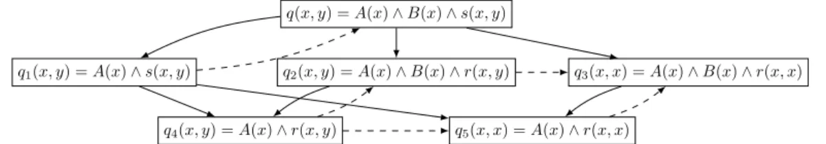
Example 4.7. Suppose that we define A and B as classes and r and s as properties. With this vocabulary, we consider the rules R1 = ∀x A(x) ⇒ B(x) and R2 = ∀x r(x, y) ⇒ s(x, y). With these rules, we can build the process rewriting graph of the query q(x, y) = A(x) ∧ B(x) ∧ s(x, y) represented by Figure 2.
q(x, y) = A(x) ∧ B(x) ∧ s(x, y)
q1(x, y) = A(x) ∧ s(x, y) q2(x, y) = A(x) ∧ B(x) ∧ r(x, y) q3(x, x) = A(x) ∧ B(x) ∧ r(x, x)
q4(x, y) = A(x) ∧ r(x, y) q5(x, x) = A(x) ∧ r(x, x)
Figure 2: The process rewriting graph of the query q(x, y) = A(x) ∧ B(x) ∧ s(x, y). The next step is to saturate the graph of rewriting process with all existing homomorphism.
Definition 4.8 (Homomorphical Saturation). The homomorphical saturation of a graph G = (V, E) whose vertices are queries, is the graph G0= (V0, E0)defined by:
• V0= V • E0= E ∪ {(q
1, q2) ∈ V2|q16= q2 and there exists a homomorphism from q1 to q2}
Example 4.9. Figure 3 represents the graph of classes of the homomorphical saturation of rewriting process graph of q(x, y) = A(x) ∧ B(x) ∧ s(x, y).
q(x, y) = A(x) ∧ B(x) ∧ s(x, y)
q1(x, y) = A(x) ∧ s(x, y) q2(x, y) = A(x) ∧ B(x) ∧ r(x, y) q3(x, x) = A(x) ∧ B(x) ∧ r(x, x)
q4(x, y) = A(x) ∧ r(x, y) q5(x, x) = A(x) ∧ r(x, x)
Figure 3: The homomorphical saturation of process rewriting graph of the query q(x, y) = A(x) ∧ B(x) ∧ s(x, y). Here, homorphisms are represented by dashed edges.
The important property of this saturation is that is allows to directly read on the obtained graph entailment (with respect to R) through reachability. This is the topic of Lemma 4.10.
Lemma 4.10. Let be G = (V, E) the homomorphical saturation of the graph of rewriting process of a conjunctive query q w.r.t. a set of existential rules R and let q1, q2 two queries in V , if q2, R |= q1, then there exists an oriented path in G from q1 to q2.
Proof. We know that q2, R |= q1, so using the Theorem 2.18 there exists q0
1 ∈ V an R-rewriting of q1 such that q2 |= q01. By definition since q0
1 is an R-rewriting of q1, there exists an R-rewriting sequence q10 = q1, q11, . . . , q
k−1 1 , q
k
1 = q10 and this sequence is an oriented path from q1 to q10 in the graph of rewriting process of q. Moreover, because q2 |= q01, there exists an edge from q0
1 to q2 in G, since G is homomorphically saturated. This proves that there is a path from q1 to q2 in G.
We now want to simplify as much as possible the obtained graph. Especially, we do not want two distinct queries of the graph to be semantically equivalent.
Definition 4.11 (Graph of Classes). Let G = (V, E) be a graph whose vertices are a subset of rewritings of the query q, ˜G = ( ˜V , ˜E)the graph of classes of G is defined by :
• ˜V is the set of semantic equivalence classes of V ; • ˜E = {(˜q1, ˜q2) ∈ ˜V2/∃(q1, q2) ∈ E2, q1∈ ˜q1, q2∈ ˜q2}
Computing the graph of classes on the homomorphical saturation amounts to merge strongly connected components, as state by the following proposition.
Proposition 4.12. Let be G = (V, E) the homorphical saturation of the graph of rewriting process of a conjunctive query q w.r.t. a set of existential rules R, the semantic equivalence class of a query q1∈ V is the strong connected component of q1 in the graph G.
Proof. We have to prove the equality between Sq1 the strong connected component of a query q1and ˜q1
the semantic equivalence class of q1in V w.r.t. R.
Let be q2 ∈ Sq1, so there is an oriented path from q1 to q2 and an oriented path from q2 to q1 in
G. By definition of edges of G and using the Corollary 2.19, we know respectively that q2, R |= q1 and q1, R |= q2, so q2∈ ˜q1.
Let be q2∈ ˜q1, so using two times Lemma 4.10 we know that there is an oriented path from q1 to q2 and the inverse path, therefore q2∈ Sq1.
Example 4.13. Using the preceding Property 4.12, we find the graph of classes of the homomorphical saturated graph from Example 4.9 reprented in Figure 4.
{q(x, y) = A(x) ∧ B(x) ∧ s(x, y), q1(x, y) = A(x) ∧ s(x, y)}
{q2(x, y) = A(x) ∧ B(x) ∧ r(x, y), q4(x, y) = A(x) ∧ r(x, y)} {q3(x, x) = A(x) ∧ B(x) ∧ r(x, x), q5(x, x) = A(x) ∧ r(x, x)}
Figure 4: The graph of classes of the homomorphical saturation of rewriting process graph of q(x, y) = A(x) ∧ B(x) ∧ s(x, y)
Last, we show that the saturated graph of R-rewriting of q can be obtained by taking the transitive reduction of the graph constructed so far. For technical simplicity, we first show that their transitive saturation are equal.
Proposition 4.14. The transitive saturation of the graph of classes of the homomorphical saturation of graph of rewriting process of a query q and of a set of existential rules R is the saturated graph of R -rewriting classes of q.
Proof. Let q be a query and R be a set of existential rules. We denote the transitive saturation of the graph of classes of the homomorphical saturation of graph of rewriting process of the query q and a set of existential rules R by GP = (VP, EP)and we denote the saturated graph of R-rewriting classes of q by GS = (VS, ES).
We only need to prove that sets of edges EP and ES are equal, because by Proposition 4.6 VP and VS are equal to the semantic classes of the set of classes of the rewritings of q with the respect of R.
First, we prove that EP ⊂ ES. As we have (C1, C2) ∈ EP, there exists an oriented path in GP from C1 to C2such as for each consecutive vertices Ca, Cb of this path, there exists qa∈ Ca and qb∈ Cb such that either:
1. qb is a R -rewriting of qa;
2. or there exists a homomorphism from qa to qb.
In both cases, we know that qb, R |= qa, so by definition of GS, we know that (Ca, Cb) ∈ ES. So the same path from C1to C2 also exists in GS and prove that C1|= C2, then (C1, C2) ∈ ES.
We want to prove the inclusion in the other way. Let (C1, C2) ∈ ES. There exists q1∈ C1and q2∈ C2 such as q2, R |= q1, so using Lemma 4.10, there is an oriented path from q1 to q2 in the homomorphical saturation of the rewriting process graph of q. So by definition of edges of GP, there is also an oriented path from C1to C2in GP. Finally, GP is a transitive saturated graph, hence (C1, C2) ∈ EP, so we prove that ES ⊂ EP.
Corollary 4.15. The transitive reduction of graph of classes of the homomorphical saturation of graph of rewriting process of a query q and of a set of existential rules R is the rewriting graph of R -rewriting classes of q.
Example 4.16. We conclude the first part of this running example by presenting the transitive reduction of Figure 4 in Figure 5. One edge has been deleted.
{q(x, y) = A(x) ∧ B(x) ∧ s(x, y), q1(x, y) = A(x) ∧ s(x, y)}
{q2(x, y) = A(x) ∧ B(x) ∧ r(x, y), q4(x, y) = A(x) ∧ r(x, y)}
{q3(x, x) = A(x) ∧ B(x) ∧ r(x, x), q5(x, x) = A(x) ∧ r(x, x)}
Figure 5: The rewriting graph of q(x, y) = A(x) ∧ B(x) ∧ s(x, y) w.r.t. rules R1= ∀x, A(x) ⇒ B(x) and R2= ∀x, r(x, y) ⇒ s(x, y).
4.2
RDFS rewriting
As the case of RDFS ontologies is especially important from a practical point of view, we introduce a method that is specifically tailored towards knowledge bases having this ontology. After a quick recall of what kind of rules are allowed within an RDFS ontology, we introduce an alterative rewriting mechanism that will be used to speed up the computation.
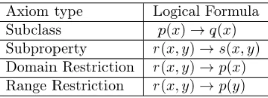
RDFS is a W3C standard [BG14] that provides a data-modelling vocabulary for RDF. More specifi-cally, it provides axioms to describe subclass, subproperty, domain and range restrictions. Expressed in a logical way, ontologies expressible in RDFS contains rules of the shape described in Table 1.
Axiom type Logical Formula Subclass p(x) → q(x) Subproperty r(x, y) → s(x, y) Domain Restriction r(x, y) → p(x) Range Restriction r(x, y) → p(y) Table 1: Axioms appearing in RDFS ontologies
The specificity of RDFS rules allows for a more simple rewriting algorithm, such as the one presented in [GMR13]. A similar rewriting method could be used as long as rules do not contain existential variables, and no variable is repeated within the head. Under these conditions, the query can be rewritten atom by atom. The algorithm for RDFS performs as well a breadth-first traversal of rewritings, but considers only unifiers µ = (q0, u)such that q0 is a single atom and where u is injective. Moreover, one can choose the names of variables introduced by the rewriting in such a way that if µ1 is applied on some atom, then µ2 on another atom, then the rewritings generated by this sequence of rewritings is syntactically the same as the one generated when rewriting first through µ2 then µ1. This can be done by assigning to each atom an integer i, and whenever an atom is rewritten, the generated atom is assigned the same integer1and if a fresh variable is introduced in that atom, one can name it F Vi, where {F Vi}
i∈Nis a set of variables disjoint from the query variables.
Example 4.17. Note that the above rewriting algorithm, despite being classically equivalent to the general rewriting algorithm, does not generate syntactically equal rewriting sets. For instance, the query q(x, y) = s(x, y), which can be rewritten by the rule r(x, y) ⇒ s(x, y), leads to different queries from a rewriting system to another:
• RDFS rewriting system allows one rewriting q0(x, y) = r(x, y),
• existential rewriting system allows two rewriting q1(x, y) = r(x, y)and q2(x, x) = r(x, x).
4.3
Product of Graph
The algorithm presented in the previous section can also be seen as follows: one compute rewritings atom by atom and then perform a cartesian product to get a rewriting of the original query. We exploit this
fact in order to compute a graph that we will use as the rewriting graph of q with respect to R. In this section, we explain Algorithm 2: we first define the output of the subroutine ComputeProductGraph (Definition 4.20), and the relationships that exist between the output of Algorithm 2 and the rewriting graph of q with respect to R. Without loss of generality, we will consider in this section that vertices of rewriting graph of a atom are queries instead of classes of queries, for simplifying notations.
Input: A conjunctive query q, a finite unification set R Output: The rewriting graph of q w.r.t. R
1 forall atom ai∈ q do
2 Gi = ComputeRewritingGraph(ai, R) 3 end
4 return Πi(Gi)
Algorithm 2: ComputeProductGraph(q, R)
Let us first introduce a generic notion of product graph.
Definition 4.18(Product Graph). Let G1, G2, . . . , Gn be graphs with Vi is the set of vertices of Gi and Ei the set of edges of Gi, G = (V, E) the product graph of G1, G2, . . . , Gn is defined by :
• V = Qn i=1Vi;
• E = {((t1, t2, . . . , tn), (u1, u2, . . . , un))/∃1 ≤ k ≤ n, (tk, uk) ∈ Ek and ∀i 6= k, ti= ui}
We directly apply this notion to the rewriting graph of atomic queries to define the product graph of a query.
Definition 4.19 (Product Graph of a Query). Let q a RDFS query defined by the atoms : a1, a2, . . . , an and G1, G2, . . . , Gn be graphs such as Gi is the rewriting graphs of ai. We define the product graph of q as the product graph of G1, G2, . . . , Gn.
With each node of the product graph of a query, we naturally associate a query.
Definition 4.20. Let G = (V, E) a product graph of a query q and (a1, a2, . . . , an) ∈ V a vertex of G, we define a query interpretation of this vertex defined as the query composed by {a1, a2, . . . , an} and the answers variables of q.
Example 4.21. Suppose that we define A and B as classes and r and s as properties. With this vocabulary, we consider the rules R1 = ∀x A(x) ⇒ B(x) and R2 = ∀x r(x, y) ⇒ s(x, y). With these rules, we want to build the product graph of the query q(x, y) = A(x) ∧ B(x) ∧ s(x, y). We first build the three rewriting graphs of the atoms of q, as shown in Figures 6, 7 and 8.
qA(x) = A(x)
Figure 6: Rewriting graph of the atomic query qA(x) = A(x)
qB(x) = B(x)
q0
B(x) = A(x)
Figure 7: Rewriting graph of the atomic query qB(x) = B(x)
qs(x, y) = s(x, y)
q0
s(x, y) = r(x, y)
Figure 8: Rewriting graph of the atomic query qs(x, y) = s(x, y) Using these rewriting graphs, we build the product graph of q and keep the repetition of atoms in vertices labels for a better understanding, in Figure 9. We notice that q and q1 are equivalentes with respect to the rules as q2 and q4.
q(x, y) = A(x) ∧ B(x) ∧ s(x, y)
q1(x, y) = A(x) ∧ A(x) ∧ s(x, y) q2(x, y) = A(x) ∧ B(x) ∧ r(x, y)
q4(x, y) = A(x) ∧ A(x) ∧ r(x, y)
Figure 9: The product graph of the query q(x, y) = A(x) ∧ B(x) ∧ s(x, y). We expect some properties of the product graph of rewriting graph of queries.
Proposition 4.22. If G1, G2, . . . , Gn are acyclic, transitively rewriting graphs, then the product graph Gof G1, G2, . . . , Gn is also acyclic and transitively reduced.
Proof. First, let v1, v2, . . . , vlbe an oriented path in G, we denote each vi= (vi
1, v2i, . . . , vin)for 1 ≤ i ≤ l. We define a projection of this path on Gk for 1 ≤ k ≤ n as the oriented path in Gk defined by the sequence of edges of Gkwhich is the maximum sub-sequence of (v1
k, v 2 k), (v 2 k, v 3 k), . . . , (v n−1 k , v n k)containing only edges of Gk. In other words, we keep from the sequence (v1
k, v 2 k), (v 2 k, v 3 k), . . . , (v n−1 k , v n k)only couples (vi k, v i+1 k )such as v i k 6= v i+1
k . We notice that the projection of the path v1, v2, . . . , vl on Gk is an empty path if and only if for all 1 ≤ i, j ≤ l we have vi
k= v j k.
We want to prove that the product graph G is acyclic. Suppose that v1, v2, . . . , vl is a cycle of G. The projection of this path on Gk for 1 ≤ k ≤ n is not empty if and only if it is a cycle in Gk. Since for all 1 ≤ k ≤ n, there is no cycle in each Gk, we know that for all 1 ≤ i, j ≤ l, we have vi
k = v j k. So v1, v2, . . . , vlis a constant sequence, but G does not contain loop by definition of these edges, absurd.
We want to prove that G is transitively reduced. We suppose the contrary by assuming the existence of an oriented path v1, v2, . . . , vl in G containing at least two edges such as (v1, vl)is an edge of G. We use the following notations v1 = (v1
1, v 1 2, . . . , v 1 n)and v l= (vl 1, v l 2, . . . , v l
n). By definition of the edges of G, there exists 1 ≤ k ≤ n such as (v1k, vlk) is an edge of Gk and ∀1 ≤ h ≤ n and i 6= k, vh1 = vlh. With this last property, we know that ∀1 ≤ h ≤ n and h 6= k, the projection of the path v1, v2, . . . , vl on Gh is empty, because otherwise there is a cycle in Gh. So for all 1 ≤ i, j ≤ l we have vi
h = v j
h. Since the path v1, v2, . . . , vl contains at least two edges, the projection of this path has to contain also at least two edges. But this projection is an oriented path in Gk from v1
k to v l
k and Gk contains the edge (v 1 k, v
l k), then Gk is not transitively reduced, absurd.
Corollary 4.23. The product graph of a query with respect to an RDFS ontology is acyclic and transitive reduced.
Proof. It follows directly from the definition of the product graph of a query.
Let us notice that the product graph thus generated is not always equal to the rewriting graph of R-rewriting classes of q, as witnessed by the Figure 10, which queries q and q1 are equivalente.
We conjecture the following proposition, which intuitively states the graph output by our optimized algorithm for RDFS is “not too far” from being the R-rewriting graph of queries of the original query. Conjecture 4.24. Let G1, G2, . . . , Gn be R-rewriting graph of queries of one atom and let G be the product graph of G1, G2, . . . , Gn. If there is t, u two vertices of G such as t, R |= u, then it exists an oriented path in the graphs of classes of G from the class of u to the class of t.
Example 4.25. A simple way to prove way to prove the Conjecture 4.24 could have to prove the following proposition. We could expect that in the product graph when there is a homomorphism from a query q1 to another q2, then there exists a homomorphism from q2 to q1. Unfortunately, this proposition is false and Figure 10 is a counter-example:
q(x) = A(x) ∧ s(x, x)
q1(x) = ∃y, s(x, y) ∧ s(x, x) q2(x) = B(x) ∧ s(x, x)
Figure 10: The product graph of the query q(x, y) = A(x)∧s(x, x) w.r.t. rules R1= ∀x, y r(x, y) ⇒ A(x) and R2= ∀x, B(x) ⇒ A(x). Dashed arrow represents an homomorphism from q1 to q2
In this example, there is a homomorphism from q1 to q2, but there is not homomorphism in the other direction.
5
Labellisation
We want to use the structure of the rewriting graph of a query q to extract from its rewritings, an interesting labellisation of q.
First we define set graphs, which extend rewriting graphs, which have the property that for a query q, each answer of q is contained in at least one leaf of the graph. We also replace semantic classes of equivalence from the vertices by one representative picked from a given function Repr which chooses a reprensentative from a class and such as if q is the original query, we have Repr(˜q) = q.
Definition 5.1(Set Graph). Let Gr= (Vr, Er)the rewriting graph of a conjunctive query q with respect to a set of existential rules R, the set graph of q with respect of R is the graph GS= (VS, ES)defined by the following equalities, where Pr is the set of vertices of Gr which have at least one child:
• VS = {Repr(C)| C ∈ Vr} ∪ {selfLeaf(C)| C ∈ Pr}
• ES= {(Repr(C1), Repr(C2))| (C1, C2) ∈ Er} ∪ {(Repr(C),selfLeaf(C))| C ∈ Pr}. where for a vertex C of Gr, we define selfLeaf(C) by:
selfLeaf(C) = Repr(C) ∧ ^ Cichild of C
¬Repr(Ci).
Proposition 5.2. Let G = (V, E) be a set graph of a conjunctive query q w.r.t. a set of existential rules Rand q1, q2two queries in V . We know that q2, R |= q1 if and only if there exists an oriented path from q1 to q2 in the set graph G.
Proof. Actually, the proposition is trivial when q1 and q2 are not selfLeaves of the set graph G. We just need to use Definition 4.2 of saturated graph and check the correctness of the proposition after each transformation of graph.
Otherwise, if there exists an oriented path from q1to q2in G, then q2is a selfLeaf and have a unique parent q2. By definition of selfLeaf, q20 |= q2, so by using the proposition for the restricted path from q10 to q2, we get the result.0
We admit that a selfLeaf does not entail using rules (which doesn’t contains negation) other queries in the set graph than queries entailed using rules by its parent. We can prove the proposition using this result.
We use the set graph to reduce the problem of finding a covering labellisation to the problem of finding a set of nodes such as each leaf has an ancestor or is itself into this set.
Proposition 5.3. Let G = (V, E) be the set graph of a conjunctive query q with respect to a set of rules R. If F is a subset of vertices of G such as for each l leaves of G it exists oriented path in G from a element of F to l, then we have the following equivalence:
q, R |= _ qf∈F
qf
Proof. We denote the set of leaves of G by LG. We have the following equations where we use Prop-erty 2.19 to go from the first to the second line and the last is obtained by applying the reasoning of the first two lines to each child of q in G.
q ≡R _ (q,q0)∈E (q ∧ q0) ∨ q ∧ ^ (q,q0)∈E ¬q0 ≡R _ (q,q0)∈E q0∨selfLeaf(q) . . . ≡R _ ql∈LG ql∨ _ qp∈V \LG selfLeaf(qp) And because LG already contains the self leaves, we have q ≡RW
ql∈LGql.
Now, for all ql ∈ LG, there exists qf ∈ F such as there is an oriented path from qf to ql. Two consecutive queries q1, q2 of this path are such as q2, R |= q1, by definition of set graph. Finally, we know that ql, R |= qf, so: _ ql∈LG ql, R |= _ qf∈F qf q, R |= _ qf∈F qf
Let D be a fact, and let R be a set of existential rules. We denote by K = (D, R) the knowledge base built out of both. We use the fact through the function answerD,R(). Let q be a non Boolean conjunctive query, answerK(q)returns the set of answers of q on D using R. In order to find a labellisation different from the set containing the initial query, we decide to set a goal t for the number of answers for labellisation queries. We want to find a labellisation which contains queries which have a number of answers as close as possible to t.
Definition 5.4 (Small Query). Let G = (V, E) a set graph of a conjunctive query q w.r.t. a set of rules Rof a knowledge base K and let be t a positive integer. The small queries St
q,K of q and K with respect to an integer t is the subset of queries of V defined by:
Sq,tK = {q0 ∈ V |#answerK(q0) < t}.
Proposition 5.5. Let G = (V, E) a set graph of a conjunctive query q w.r.t. a set of rules R of a knowledge base K and let be t a positive integer. If a vertex of G, qsis in St
q,K (resp. qbis not in S t q,K), then all descendants of qs (resp. all predecessors of qb) in G are in St
G (resp. not in S t G). Proof. Suppose that qs∈ St
q,K and qk ∈ V is a descendant of qssuch as q0= qs, q1, . . . , qk is an oriented path in G. According to Property 5.2, we know that qk, R |= qs. So we have the following implications:
qk, R |= qs ⇒ answerK(qk) ⊂ answerK(qs) ⇒ #answerK(qk) ≤ #answerK(qs) ⇒ #answerK(qk) < t
⇒ qk∈ St q,K The proof is similar for qb∈ S/ t
q,K.
We define the notion of border in a set graph in order to get a such labellisation.
Definition 5.6 (Frontier). Let G = (V, E) a set graph of a conjunctive query q w.r.t. a set of rules R of a knowledge base K and be a positive integer such as t ≤ #answerK(q). The frontier Fq,tK of q and K with respect to t is the set of queries defined by:
Fq,tK = Vs∪ Vb, where Vs= {qs|qs∈ St q,K and ∀(q 0, qs) ∈ E, q0∈ S/ t q,K} and Vb= {qb|qb∈ S/ tq,K and ∀(qs, q0) ∈ E, q0∈ S t q,K}
Definition 5.7 (Big Frontier). Let G = (V, E) a set graph of a conjunctive query q w.r.t. a set of rules R of a knowledge base K and be a positive integer such as t ≤ #answerK(q). The big frontier BFt
q,K of q and K w.r.t. t is the set defined by:
BFq,tK = Fq,tK \ {qs|(qs, qb) ∈ (Ft q,K)
2∩ E}
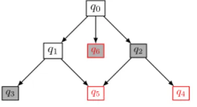
Example 5.8. We illustrate the big frontier on the set graph drawn on Figure 11. In this figure, red vertices are representing small vertices, black vertices the rest of them. Vertices that are gray filled are the vertices of the big frontier.
q0
q1 q2
q3 q5 q4
q6
Figure 11: Example of big frontier defined vertices filled in grey, where small queries are in red and others queries in black.
Definition 5.9 (Small Frontier). Let G = (V, E) a set graph of a conjunctive query q w.r.t. a set of rules R of a knowledge base K and be a positive integer such as t ≤ #answerK(q). The small frontier of q and K with respect to a integer t is the set defined by:
Fq,tK \ {qb|(qs, qb) ∈ (Fq,tK) 2
Proposition 5.10. Let G = (V, E) a set graph of a conjunctive query q w.r.t. a set of rules R of a knowledge base K and be a positive integer such as t ≤ #answerK(q). The small frontier and big frontier BFt
q,K of q and K with respect to t is a simple labellisation of G.
Proof. Suppose that we have q1and q2two vertices of the big (or small) frontier of G, such as q2, R |= q1. According to Property 5.2, we know that there exists an oriented path from q1 to q2 in G. If q1∈ St
q,K, then we know that all descendants of q1 in G are in St
q,K by Property 5.5, in particular q2∈ Sq,tK. Also if q1∈ S/ t
q,K, then since q1∈ F t
q,K, all children of q1are in S t
q,K, by extension all descendants of q1 and in particular q2 ∈ St
q,K. In all cases q2 ∈ S t
q,K, since q2 is also in q2 ∈ F t
q,K, so for same reasons as preceding, all predecessors of q2 are not in St
q,K and q2∈ S/ q,tK. We know that all descendants of q1 are in St
q,K and all predecessors of q2are not in Sq,tK, so (q1, q2) ∈ E ∩ (Fq,tK)2. By definition of the big (or small) frontier, it is impossible.
Proposition 5.11. Let G = (V, E) a set graph of a conjunctive query q and t be an integer such as t ≤ #answerK(q). The small frontier and the big frontier of q and K with respect to t are covering labellisations of G.
Proof. We expose a proof for the big frontier denoted by Ft
q,K, which is also correct for the small frontier, until we distinguish both cases.
According to the Proposition 5.3, we just need to prove that for each leaf qlof the set of leaves LG of G, there exists an ancestor of ql in Ft
q,K. It implies that F t
q,K is a covering labellisation of G. Let ql be a leaf of G, we know that if ql ∈ S/ t
q,K, then ql ∈ Fq,tK, because ql has no child. In the other case ql∈ St
q,K then it exists an ancestor qa ∈ S t
q,K of qlsuch as qa has no parent in S t
q,K, because q /∈ St
q,K and G is acyclic. By definition, we know that qa is in the border of G w.r.t t. If Ft
q,K is the small frontier, then qa ∈ Fq,tK, else Fq,tK is the big frontier and we know that either: • qa has no parent in the frontier, hence qa∈ Ft
q,K
• or qa has a parent in the frontier, hence this parent is in Ft q,K. In all cases, we have found a ancestor of ql in Ft
q,K.
The building of the set graph from a product graph can be done by reuse Definition 5.1. With a set graph based on a product graph each result of this section holds, if Conjecture 4.24 is true. But the fact that the big (or small) frontier is covering holds anyway in both cases.
6
Implementation & Experiment
We describe in this section the implementation and experiments that have been led to validate our approach. We first tried a direct implementation of Algorithm 1, on which we intented to run our labellisation technique. As will be clear from the experiments, this approach proved to be too slow to be relevant. This motivated the optimization we developed for RDFS, as our test ontologies are expressed in this ontology language. The first set of experiments we present is thus focused on the computation of the rewriting graph of R-rewritings, showing that the product graph approach leads to improved performance. Evaluating the quality of the output labellisations is a task that is much more complicated, and out of the scope of this paper (more on this in the future work section). We still performed a “soundness check”, by running our algorithm on several queries on DBPedia and checking the output seemed “reasonable”.
6.1
Resources
6.1.1 Datasets
We conducted experiments on two datasets:
• LUBM, which is classically used in the evaluation of ontology-based query answering. LUBM is a synthetic dataset, that is equipped with an ontology. The ontology exists in several flavors, and we consider here the RDFS version. A set of queries is also provided.
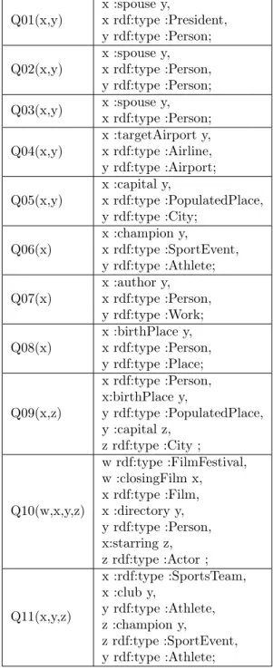
• DBPedia 2 is a knowledge base which is built from the information created in the Wikipedia project. The ontology is much richer than the LUBM one, while being still expressible in RDFS. We handcrafted a set of queries, presented in Annex A.
While LUBM is the classical experiment dataset in our setting, we judged it was not very interesting from a point of view of query answers exploration, as the ontology is rather flat and the data is synthetic. DBPedia avoids these two shortcomings, and will allow for better future integration with other semantic web resources.
6.1.2 Implementation
Our prototype relies on RDF-Commons3, which is a library that has been developed within the Cedar (and previously OAK) team. More specifically, this library provides us with data storage, query repre-sentation, query reformulation and query evaluation capabilities.
6.2
Computation of the Rewriting Graph
In this experiment, we aim at comparing the time needed to compute the rewriting graph with Algorithm 1, or its approximation with the optimization for RDFS. We also evaluate the quality of the approximation. We define dedicated a set of queries on DBPedia accessible in Table 2 in annex.
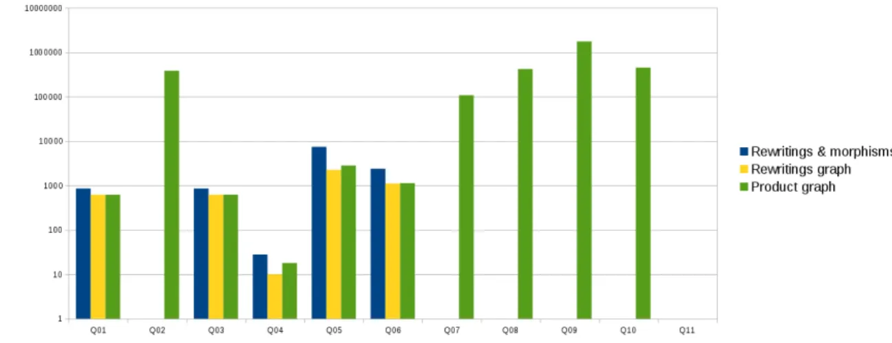
First, we want to evaluate and compare the effectiveness of the two methods we propose for building a graph containing the rewritings. Figure 12 shows that the execution time to build rewriting graph is slower than product graph, except for query Q04. For some queries like Q02, Q07, Q08, Q09, Q10, Q11, rewriting graph building is not finished after 30 minutes. The execution of the both methods on query Q11 fails to finish before this timeout. Times of executions for rewriting graph building is splited into times of the three following operations:
1. Rewritings & morphisms corresponds to Lines 4 to 18 of Algorithm 1 and to the building of homo-morphical saturation of the process graph,
2. Graph of classes corresponds strongly connected components merging at Line 21, by Merge-StronglyConnectedComponents of Algorithm 1,
3. Transitive reduction corresponds to transitive reduction computed by TransitiveReduction function of the same algorithm.
Figure 12: Comparaison of building times of the rewriting graph and product graph. Rewriting graph times are splited into each of step of the algorithm.
In order to compare also the quality of the output of the product graph approximation with the exact rewriting graph, we show the number of vertices in Figure 13 and the number of edges in Figure 14 of both methods. We also add to each figure the output value after each steps of the rewriting graph method, if the value changes during this step. We notice that when the both end before the timeout, the number of vertices and edges of product graph is quite comparable with those of the rewriting graph. The small size of the output for query Q04 may explain the fact that product graph building is slower than that of the rewriting graph.
6.3
Building Labellisations
In this part, we aim to illustrate the output of the labellisation algorithm. We choose to implement a method to build the big frontier from a set graph or rewriting graph.
Figure 13: Comparaison of number of vertices of rewriting graph and product graph.
Figure 14: Comparaison of number of vertices of rewriting graph and product graph.
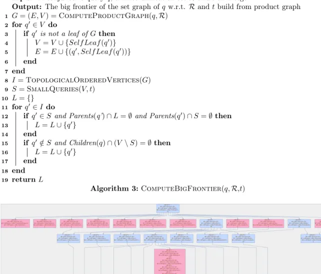
Algorithm 3 defines how we build the set graph from the product graph of a query and a set of rules and how we extract of it the big frontier w.r.t. of an integer. From Line 2 to 6, we increase the product graph with selfLeaf to construct a set graph. We build a topological ordered list of the vertices of set graph at Line 8. Then we browse vertices of set graph to extract the big frontier between Line 11 to Line 17.
We also run labellisation algorithm with a parameter t = 9 on the query q(x, y) = x rdf:type :Politician, x :spouse y, y rdf:type :Artist. There are 47 answers for q into DBpedia. Its product graph contains 945 vertices and 1812 edges. The labellisation contains 12 queries, including one selfLeaf, including:
• q1(x, y) = ∃z, xrdf:type :President, x :spouse y, z :starring y; • q2(x, y) = ∃z, xrdf:type :Politician, x :spouse y, y :field z;
• q3(x, y) = xrdf:type :Congressman, x :spouse y, y rdf:type :Artist; • q4(x, y) = xrdf:type :Politician, x :spouse y, y rdf:type :MusicalArtist; • q5(x, y) = ∃z, xrdf:type :Politician, x :spouse y, y :movement z.
We display at Figure 15 the explored part of set graph of q during the labellisation process. The selfLeaf of the labellisation has a long label and 13 answers. It has both an important cardinality (for this example) and a label which is diffcult to apprehend.
7
Future Work
Input: A conjunctive query q, a finite unification set R and t an integer
Output: The big frontier of the set graph of q w.r.t. R and t build from product graph 1 G = (E, V ) = ComputeProductGraph(q, R)
2 for q0∈ V do
3 if q0 is not a leaf of G then 4 V = V ∪ {Self Leaf (q0)} 5 E = E ∪ {(q0, Self Leaf (q0))} 6 end 7 end 8 I = TopologicalOrderedVertices(G) 9 S = SmallQueries(V, t) 10 L = {} 11 for q0∈ I do
12 if q0∈ S and Parents(q’) ∩ L = ∅ and Parents(q0) ∩ S = ∅ then 13 L = L ∪ {q0}
14 end
15 if q0∈ S/ and Children(q) ∩ (V \ S) = ∅ then 16 L = L ∪ {q0}
17 end 18 end 19 return L
Algorithm 3: ComputeBigFrontier(q, R,t)
Figure 15: Explored part of set graph of query q(x, y) = x rdf:type :Politician, x :spouse y, y rdf:type :Artist during the labellisation process, except ver-tices have a not empty answers set. The verver-tices of the labellisation appear in pink.
Evaluation As already mentioned, evaluating the quality of the labellisation algorithm is an important and non-trivial task, as the aim is to ease the grasp of answer sets by human users. Setting such an experiment is a non-trivial task and was out of the scope of this internship. A lighter way of evaluating the interest of such an approach would be to disseminate (an upgraded version) of the tool developed in the internship to get feedback on the interest of the proposed labellisations.
Exploring the Space of Labellisation Strategies The algorithm that we propose is in some sense data oblivious: data is only used to chose labels among queries that are generated, but it has no influence on the set of labels that are considered. While this has some advantages with respect to the running time of the algorithm, it significantly reduces the insights that such a technique can provide. A systematic description of labellisation strategies together with algorithms illustrating each strategy would be very beneficial.
Control of the labellisation size The initial idea behind the labellisation was to sum up the answers by using semantics labels defining interesting subsets of answers. But our method has no way to control the number of labels contained in the labellisation. In order to return an apprehendable labellisation, it could be relevant to control or limit the number of labels. One way to achieve this is to consider a
distance on the labels for clustering the actual labellisation.
Optimization A substantial part of the presented work consists in optimizing the creation of the rewriting graph of R-rewritings, exploiting the fact that there are interesting ontologies available whose expressivity is rather weak. As seen in the experiments, even optimized some realistic queries do not allow for a quick computation of that graph. A way to avoid that problem would be to compute only parts of the graph, refining only the parts that are necessary when considering the query answers. The second step is also prone to optimization, as queries that are evaluated usually share high commonalities, leaving the space for the use multi query optimization techniques.
Rules Generalization We define a method to get a labellisation from a set of rules and a query, such as we know that the set of rewriting queries is finite. Some sets of rules are such as for each queries there exists a finite subset of its rewritings satisfying Theorem 2.18 as the all set of its rewritings. Even if a covering and simple labellisation can be extracted from rewritings in this context, the building of the rewriting graph can be infinite. It will be interesting to generalize the rewriting graph in order to cope with this context.
References
[BCM+03] F. Baader, D. Calvanese, D. L. McGuiness, D. Nardi, and P. Patel-Schneider, editors. The Description Logic Handbook. Cambridge University Press, 2003.
[BG14] D. Brickley and R.V. Guha. RDF Schema 1.1. Technical report, W3C, Feb 2014.
[BLMS11] Jean-François Baget, Michel Leclère, Marie-Laure Mugnier, and Eric Salvat. On rules with existential variables: Walking the decidability line. Artif. Intell., 175(9-10):1620–1654, 2011. [CGK13] Andrea Calì, Georg Gottlob, and Michael Kifer. Taming the infinite chase: Query answering
under expressive relational constraints. J. Artif. Intell. Res., 48:115–174, 2013.
[CGP10] Andrea Calì, Georg Gottlob, and Andreas Pieris. Query answering under non-guarded rules in datalog+/-. In Web Reasoning and Rule Systems - Fourth International Conference, RR 2010, Bressanone/Brixen, Italy, September 22-24, 2010. Proceedings, pages 1–17, 2010. [DHS00] R. O. Duda, P. E. Hart, and D. G. Stork. Pattern Classification (2Nd Edition).
Wiley-Interscience, 2000.
[GMR13] François Goasdoué, Ioana Manolescu, and Alexandra Roatis. Efficient query answering against dynamic RDF databases. In Joint 2013 EDBT/ICDT Conferences, EDBT ’13 Proceedings, Genoa, Italy, March 18-22, 2013, pages 299–310, 2013.
[IBS08] I. F. Ilyas, G. Beskales, and M. A. Soliman. A survey of top-k query processing techniques in relational database systems. ACM Comput. Surv., 40(4), 2008.
[LIJ+15] J. Lehmann, R. Isele, M. Jakob, A. Jentzsch, D. Kontokostas, P. N. Mendes, S. Hellmann, M. Morsey, P. van Kleef, S. Auer, and C. Bizer. Dbpedia - A large-scale, multilingual knowl-edge base extracted from wikipedia. Semantic Web, 6(2):167–195, 2015.
[MBS15] F. Mahdisoltani, J. Biega, and F. M. Suchanek. YAGO3: A knowledge base from multilin-gual wikipedias. In CIDR 2015, Seventh Biennial Conference on Innovative Data Systems Research, Asilomar, CA, USA, January 4-7, 2015, Online Proceedings, 2015.
[MT14] Marie-Laure Mugnier and Michaël Thomazo. An introduction to ontology-based query an-swering with existential rules. In Reasoning Web, pages 245–278, 2014.
[vHLP07] Frank van Harmelen, Vladimir Lifschitz, and Bruce Porter. Handbook of Knowledge Repre-sentation. Elsevier Science, San Diego, USA, 2007.
[VK14] Denny Vrandečić and Markus Krötzsch. Wikidata: A free collaborative knowledgebase. Com-mun. ACM, 57(10):78–85, September 2014.
Annex A
Q01(x,y) x :spouse y,x rdf:type :President, y rdf:type :Person; Q02(x,y) x :spouse y,x rdf:type :Person, y rdf:type :Person; Q03(x,y) x :spouse y,x rdf:type :Person; Q04(x,y) x :targetAirport y,x rdf:type :Airline, y rdf:type :Airport;
Q05(x,y) x :capital y,x rdf:type :PopulatedPlace, y rdf:type :City;
Q06(x) x :champion y,x rdf:type :SportEvent, y rdf:type :Athlete; Q07(x) x :author y,x rdf:type :Person,
y rdf:type :Work; Q08(x) x :birthPlace y,x rdf:type :Person,
y rdf:type :Place; Q09(x,z) x rdf:type :Person, x:birthPlace y, y rdf:type :PopulatedPlace, y :capital z, z rdf:type :City ; Q10(w,x,y,z) w rdf:type :FilmFestival, w :closingFilm x, x rdf:type :Film, x :directory y, y rdf:type :Person, x:starring z, z rdf:type :Actor ; Q11(x,y,z) x :rdf:type :SportsTeam, x :club y, y rdf:type :Athlete, z :champion y, z rdf:type :SportEvent, y rdf:type :Athlete;