HAL Id: tel-03215837
https://tel.archives-ouvertes.fr/tel-03215837
Submitted on 3 May 2021HAL is a multi-disciplinary open access archive for the deposit and dissemination of sci-entific research documents, whether they are pub-lished or not. The documents may come from teaching and research institutions in France or abroad, or from public or private research centers.
L’archive ouverte pluridisciplinaire HAL, est destinée au dépôt et à la diffusion de documents scientifiques de niveau recherche, publiés ou non, émanant des établissements d’enseignement et de recherche français ou étrangers, des laboratoires publics ou privés.
du mercure dans l’hémisphère Sud
Chuxian Li
To cite this version:
Chuxian Li. Variabilité Holocène des poussières atmosphériques et du mercure dans l’hémisphère Sud. Océan, Atmosphère. Université Paul Sabatier - Toulouse III, 2019. Français. �NNT : 2019TOU30277�. �tel-03215837�
THÈSE
En vue de l’obtention du
DOCTORAT DE L’UNIVERSITÉ DE TOULOUSE
Délivré par l'Université Toulouse 3 - Paul Sabatier
Présentée et soutenue par
Chuxian LI
Le 17 septembre 2019
Variabilité Holocène des poussières atmosphériques et du
mercure dans l'hémisphère Sud
Ecole doctorale : SDU2E - Sciences de l'Univers, de l'Environnement et de l'Espace
Spécialité : Surfaces et interfaces continentales, Hydrologie Unité de recherche :
ECOLAB - Laboratoire d'Ecologie Fonctionnelle et Environnement Thèse dirigée par
François De Vleeschouwer et Jeroen SONKE Jury
M.Dominic Hodgson, Rapporteur
M.Jiubin Chen, Rapporteur
Mme Mattielli Nadine, Examinatrice M. Gaël Le Roux, Examinateur Mme Catherine Jeandel, Invitée
M.De Vleeschouwer François, Directeur de thèse
221
Abstract
The Southern westerly winds (SWW) play an important role in regulating Southern Ocean carbon budget by enhancing the absorbance of atmospheric CO2 or resurfacing deep ocean
carbon. Changes in SWW intensity are thought to determine whether Southern Ocean acts as a net CO2 sink or source, thereby affecting atmospheric CO2 concentration and then global
climate. SWW also affect Southern Hemisphere (SH) dust trajectory and mercury biogeochemical cycling, which in turn can be used to trace SWW dynamics. Less is known about the past SWW variabilities and historical mercury cycle. The aim of this PhD study is to improve our understanding of the SWW trend and mercury deposition in the Holocene at remote SH sites by using geochemical and isotopic proxies in peat archives. We investigated Amsterdam Island (AMS) peat record coupled with three other peatlands in the SH mid latitudes as long-term archives of atmospheric dust and/or mercury deposition. At the northern edge of SWW and free from anthropogenic disturbance, AMS is a key site to study SWW dynamics. We find that during the Holocene, dust and mercury deposition at AMS oscillated on millennial time scales. Mercury isotope signatures, which are sensitive to rainfall inputs, indicate that high dust, high mercury events correspond to low rainfall. We suggest that these events were caused by a poleward shift of the SWW at AMS. The peat mercury records also inform on recent, human perturbation of the natural mercury cycle in the SH. We find however that the 4-fold anthropogenic mercury enrichment we observe in the SH since 1450AD, is smaller than the 16-fold enrichment in the northern hemisphere. These scientific contributions should help improve global climate models and international environmental policy under the Minamata convention on mercury.
4
Résumé
Les vents de sud-ouest (VSO) de l'hémisphère sud (HS) régularisent les cycles biogéochimiques du carbone de l'océan Austral en augmentant l'absorption du CO2
atmosphérique ou en faisant remonter les éléments nutritifs et le carbone des profondeurs de l'océan. Les changements d'intensité des VSO déterminent si l'océan Austral agit comme un puits ou une source nette de CO2, affectant ainsi la concentration de CO2 atmosphérique et donc
le climat. Les VSO régularisent également la trajectoire des poussières dans l’HS et le cycle biogéochimique du mercure, ces deux paramètres pouvant donc être utilisés en retour pour suivre la dynamique des VSO. Or, les variabilités des VSO passées et sur le cycle historique du mercure sont mal connus. L'objectif de cette étude doctorale est d'améliorer la compréhension de la dynamique des VSO et du Hg atmosphérique d’abord dans un contexte de variabilité climatique naturelle puis sur une période affectée par le changement global en HS. Nous avons étudié l'enregistrement de la tourbe de l'île d'Amsterdam (AMS) ainsi que de trois autres tourbières situéesaux latitudes moyennes de l'SH, comme archives à long terme de la poussière atmosphérique et/ou du dépôt de mercure. A la limite nord des VSO et libre de perturbation anthropique, AMS est un site clé pour l'étude de la dynamique des VSO. Nous avons révélé qu’au cours de l'holocène, les dépôts de poussières et de Hg à AMS ont oscillé sur des échelles de temps millénaires. Les signatures isotopiques du Hg, sensibles aux précipitations, indiquent que des épisodes de fortes concentrations de poussières et de Hg correspondent à de faibles précipitations. Nous suggérons que ces événements ont été causés par un transfert polaire du VSO à AMS. Les dépôts de Hg reconstruits montrent également que le quadruplement du Hg anthropique observé dans l’HS depuis 1450 reste inférieur à l'enrichissement dans l'hémisphère nord, multiplié par 16 pendant la même période. Ces contributions scientifiques permettront d’améliorer les modèles climatiques et la politique environnementale internationale dans le cadre de la convention de Minamata sur le Hg.
5
Extended abstract
The Southern westerly winds (SWW) are one of the main Southern Hemisphere (SH) climatic features, which regulate the Southern ocean carbon sink, mercury (Hg) biogeochemical cycles and dust trajectories from Southern South America, Southern Africa and Australia. Changes in SWW intensity are thought to determine whether Southern Ocean acts as a sink or source of CO2, therefore affecting atmospheric CO2 concentration and then
global climate. Less is known about the long-term SWW variabilities, which hampers a thoroughful assessment on the relationship between SWW dynamics and atmospheric CO2.
Atmospheric dust deposition to mid-latitude SH records information of SWW dynamics. Atmospheric Hg mainly exists as gaseous elemental Hg (Hg0, >95%), which has a long
atmospheric lifetime (months), allowing its hemispheric dispersion before deposition to the Earth’s surface, including remote areas. Hg has seven stable isotopes that fractionate both mass dependently (MDF) and mass independently (MIF) during source mixing and Hg transformation. Hg even-isotope MIF (reported as Δ200Hg) is conservative in the Earth’s surface environment, with distinct signatures in different Hg deposition end-members (rainfall HgII and gaseous Hg0). This gives an insight to investigate the SH mid-latitude Hg rainfall HgII deposition and subsequently the principal climate driver, SWW. Hg is a toxic element. The extent of anthropogenic Hg enrichment in the SH relative to the natural background period (<1450AD, before large-scale Spanish mining) remains unclear.
This PhD research focuses on the SWW variabilities in the Holocene and historical Hg deposition by studying the time-series variations of two atmospheric proxies, dust and Hg, both of which can derive from natural and anthropogenic emissions. Natural peat deposits can be used as archives of past atmospheric dust and Hg deposition. Peat bogs are exclusively fed by atmospheric input and therefore ideal atmospheric recorders. We principally use a peat bog profile from Amsterdam Island (AMS) as a main historical archive, coupled with three other bogs from the Falkland Islands (Islas Malvinas), and Tierra del Fuego (Argentina). AMS, located at the northern edge of SWW, is sensitive to the change in wind intensity.
In this thesis, Chapter 1 estabilishes a robust chronology for the AMS peat core and shows distal dust input to AMS peatland. Chapter 2 quantifies the amount of dust input to AMS peat from different potential sources and shows oscillated SWW at the northern edge of the wind belts in the Holocene. Chapter 3 attemps to develop a new SWW proxy by using mercury
6
isotopes. Chapter 4 focuses on historical mercury deposition, which highlights that atmospheric background Hg levels in the NH and SH are different.
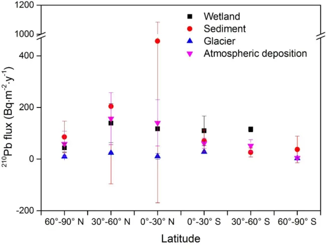
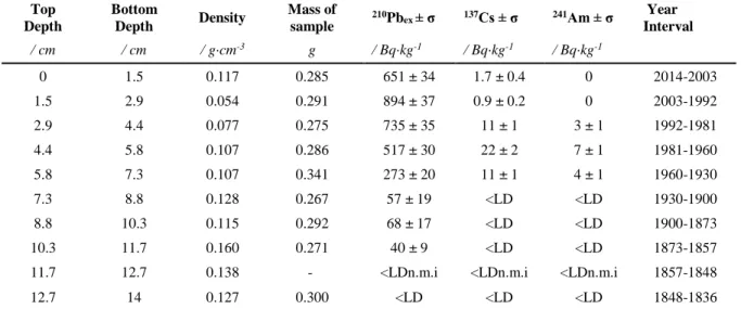
AMS recent peat chronology is established by the 210Pb Constant Rate of Supply (CRS) model, which is validated by peaks of artificial radionuclides (137Cs and 241Am) that are related to nuclear weapon tests. The AMS 210Pb flux results coupled with an updated global 210Pb data compilation show that an important quantity of continental dust is deposited over this island (Chapter 1). Using REE and Nd isotope mass balance calculations, we find Southern South America as a dominant atmospheric dust contributor (~45%) to AMS over the past 6.6 kyr. Local AMS dust sources contribute 40%, while Southern Africa contributes the remaining 15% (Chapter 2). Two mineral dust flux minima occur during 6.2-4.9 cal. kyr BP and 3.9-2.7 cal. kyr BP, interpreted as periods with equatorward-shifted and/or strengthened SWW at its northern edge. These interpretations are based on higher wind speeds leading to removal of distal dust on the way to AMS, by turbulence and enhanced wet deposition. We find that AMS peat Δ200Hg, a proxy for rainfall Hg, covaries with low dust and low Hg deposition and is in
agreement with the dust-based SWW variability (Chapter 3). Our results, therefore, give the first insight to use Hg isotopes as a climatic rainfall paleoproxy.
Recent peat layers show larger, 1.0‰, Δ199Hg variability from mid-19th to mid-20th
centuries that could reflect changes in the isotopic composition of the SH atmospheric Hg pool in response to growing industrial emissions and/or changes in Hg photochemistry (Chapter 3). Our study also shows a doubling of the Southern African dust contribution to AMS in the last 100 years relative to the long past (Chapter 2). This recent shift in dust provenance is not accompanied by enhanced dust deposition at AMS. We therefore suggest that land degradation, agriculture and dryer climate conditions in Southern Africa have led to enhanced dust mobilization in the last 100 years.
Four SH peat Hg profiles have contributed to the under-represented SH Hg dataset, showing a x3 increase in atmospheric Hg deposition since pre-industrial times (1450-1880AD). After reviewing 18 other SH sediment and 3 peat core, and updating the NH historical Hg peat and sediment database, we find that the all-time Hg increase (from pre-1450AD to 20th century) is x16 in the NH and x4 in the SH (Chapter 4). We attribute this difference to a combination of lower anthropogenic Hg emissions in the SH, and higher marine SH Hg emissions, supported by x2 higher natural background Hg accumulation in the SH peat. Our findings suggest that background Hg levels in both hemispheres are different and should be taken into account in international Hg assessment reports and environmental policy objectives.
7
Résumé étendu
Les vents du Sud-Ouest (VSO) sont l'une des principales caractéristiques climatiques de L’hémisphère Sud (HS). Ils régulent le puits de carbone de l'océan Austral, les précipitations et les trajectoires de poussières des latitudes moyennes du Sud de l'Amérique du Sud, de l'Afrique australe et de l'Australie. Les dépôts de poussières atmosphériques sur les continents et les îles de l’HS incorporent à leur tour des informations sur la dynamique des VSO. Le mercure atmosphérique existe principalement sous forme de Hg élémentaire gazeux (Hg0,> 95%), d’une durée de vie suffisamment longue (6-12 mois) dans l’atmosphère pour permettre sa dispersion hémisphérique avant son dépôt à la surface terrestre, y compris dans des régions éloignées. L'ampleur de l'enrichissement anthropique en Hg dans l’HS par rapport à la période naturelle de référence reste incertaine (<1450AD, avant l'extraction minière à grande échelle en Espagne). Le Hg est caractérisé par sept isotopes stables dont les masses fractionnent de façon dépendante (MDF) et indépendante (MIF) lors des transformations du Hg. Le MIF du Hg à isotopes pairs (rapporté par Δ200Hg), qui résulte de réactions photochimiques en haute
atmosphère, présente des signatures distinctes selon le mode de dépôt (précipitations HgII et Hg0 gazeux). Les dépôts de tourbe peuvent être utilisés comme archives des dépôts de poussières atmosphériques et du mercure (Hg) au cours de l’Holocène.
Cette thèse de doctorat porte sur les variations de deux variables atmosphériques au cours de l’Holocène et dans l’Hemisphéère Sud: les poussières et le Hg, pouvant toutes deux provenir d'émissions naturelles et anthropiques. Les tourbières sont exclusivement alimentées par les apports atmosphériques et sont donc des enregistreurs atmosphériques idéaux. Nous avons principalement étudié un profil de tourbière bien daté de 6.6 kyr de l'île d'Amsterdam (AMS, Océan Indien, extrémité nord-ouest de VSO), ainsi que de trois tourbières des îles Malouines et de Terre de Feu (Argentine).
Nos résultats de 210Pb à AMS, associés à une compilation de données 210Pb globale actualisée, montrent qu'une quantité importante de poussières continentales se dépose sur cette île (Chapter 1). En utilisant les calculs du bilan de masse à partir des données des terres rares (REE) et des isotopes du Nd, nous trouvons que l’Amérique du Sud contribue pour environ 45% à ces dépôts de poussière atmosphérique sur l’AMS au cours des derniers 6,6 kyr (Chapter 2). La contribution de l’Afrique Australe s’élève à 15%, tandis que les sources de poussières
8
locales d’AMS représentent 40%. Deux périodes de flux minimal de poussières minérales sont enregistrées entre 6.2 et 4.9 kyr BP et 3.9-2.7 cal. kyr BP, et interprétées comme des périodes de mouvement équatorial et/ou de renforcement des VSO à leur limite nord. Ces interprétations sont basées sur des vitesses de vent plus élevées conduisant à l’élimination de la poussière distale sur son trajet menant à AMS, par turbulence et augmentation du dépôt humide. Nous constatons que le Δ200Hg (témoin de dépôt humides du Hg) enregistré à dans la tourbe de AMS correspond à un faible dépôt de poussières et de Hg (Chapter 3). Ceci est en accord avec la variabilité des VSO basée sur les poussières. Nos résultats offrent donc un premier aperçu de l’utilisation des isotopes du Hg en tant que paléoproxy des précipitations climatiques. Notre étude montre un doublement de la contribution de la poussière d’Afrique Australe à AMS au cours des 100 dernières années. Cette augmentation récente ne s'accompagne pas d'un accroissement du dépôt de poussière global. Nous suggérons donc que la dégradation des sols, l'agriculture et les conditions climatiques plus sèches en Afrique Australe ont conduit à une augmentation de la taille des zones sources mobilité accrue de la poussière.
Les profils de Hg des quatre tourbières de cette étude contribuent à la base de données globale du mercure en apportant un nombre conséquent de nouvelles données pour l’HS. Nos données montrent un triplement des dépôts atmosphériques de Hg depuis l’ère préindustrielle (1450-1880AD). Après avoir examiné 18 sondages sédimentaires et 5 de tourbe de l’HS, et mis à jour la base de données historique de l’HN, nous pouvons montrer que l'augmentation absolue du Hg (d'avant 1450AD au 20ème siècle) est d’un facteur 16 dans l’HN et 4 dans l’HS (Chapter 4). Nous attribuons cette différence à une combinaison d'émissions anthropiques de Hg plus faibles dans le SH, et d'émissions marines de Hg plus élevées dans le SH, soutenues par une accumulation de Hg de fond naturel x2 plus élevée dans la tourbe du SH. Nos conclusions suggèrent que les niveaux atmosphériques de Hg dans les deux hémisphères sont différents et doivent être pris en compte dans les rapports internationaux d'évaluation du Hg et la politique environnementale internationale en appuie de la Conventions de Minamata sur le Hg.
9
Acknowledgements
Looking back for the past four years, I am so grateful for what I have had and who I have met. I am just lucky, lucky to have two excellent supervisors, an amazing mentor, two great committee members, two good teams and many nice friends! My PhD life is, awesome!
Before I started my PhD life, a little bird told me that it was more difficult to have nice supervisors than to win a lottery. When I met François and Jeroen, I knew I hit the jackpot. Both of them are brilliant and patient. They are often there to supervise me in lab work, presentation, scientific writing and of course how to conduct good scientific research. In the first half of my PhD, I mainly stayed in Ecolab and worked with François. Apart from academic teaching in science, Francois also shows me how to enjoy life. When we travelled together to Poland, Argentina, Chile, China and Spain for field trips and conferences, he never stopped exploring the local cuisine when we finished work. François is also an excellent cook, from which I have benefited a lot in the first two years of my PhD! Once François told me, “Take it seriously for science, but take it easy for life.” I think I will never forget about it.
I moved my office to GET to work with Jeroen when François was on secondment to Argentina last year. I still remember the frequency that I went to knock at the door of Jeroen’s office for discussions on my work (at least 4 times per week). Jeroen is a super busy researcher with plenty of scientific and administrative responsibility. But he always spares his time for me, helping me better understand how science works and guiding me to think about science in a different but exciting way. For example, the first draft of my abstract to ICMGP 2019 was pale and boring. It was Jeoren’s suggestions and comments that inspired me to improve it to a very interesting version. In addition, Jeoren’s way of expression is always straight to the point and enlightening. The discussions with him can always give me deeper insights about my work and other science. Both Jeroen and François are easy going and open minded. It is so comfortable and exciting to work with them!
So far, I have known some part of French culture pretty well, especially about the wine, fromage and magret de canard. Most of my French knowledge are gained from Catherine and her family (Hugo, Jane and Rémi). Catherine is my mentor for life and science. She is the best mentor I have ever had by far. When I think about Catherine at this moment, the song “You raise me up” just come to my mind. There are countless times that my soul was weary during my PhD period and Catherine was always there for me, giving me courage and love, like a parent. “She is so wise, intelligent and kind”, said my parents after they met in my hometown
10
in Guangdong province, China. I cannot agree more. I have openly and secretly learned so many things from her. For example, she always respects people regardless of their backgrounds. I have seen so many times that she helped refugees and uneducated persons to make a better life. She is very good at conducting public science, such as, le train du climat. To do public science is part of my future projects. I think I have gained some inspirations and ideas from her these years.
The luckiest thing during my PhD life is that I have lived with Catherine and her family in a super cozy house since my arrival in France four years ago. They keep teaching me French all the time, especially Rémi, who speaks French so elegantly. One of the most exciting and interesting things to live in this house is that they cook various type of cuisine every day, which is absolutely delicious. Like Francois, Hugo and Catherine are also fantastic cooks. Hugo can not only make the dishes excellent in taste but also in looks. Jane excels in making desserts, especially chocolate cake and Tiramisu! It is a shame that I still don’t know how to cook good French cuisine because I always prefer washing the dishes than cooking. But I guess I will follow the family’s recipes during my post-doc. All these good times with the family support me to work efficiently for my research in science.
I have travelled to many countries for conferences and meetings by far. One fourths of the trips are funded by Gaël Le Roux, the head of BIZ team in Ecolab. Gaël is very smart and contributes a lot to improve my PhD study. He often guides me to think in a global scale in research. I had no clue how he was capable of possessing a global view of various scientific fields even including the ones out of his specialized areas, until we attended the conference SIL 2018 in Nanjing, China together. I found out that he liked attending the keynote talks from different disciplines. He told me that those big names who gave keynotes would always give you an expert’s view from a different field, from which we could learn many other sciences. What a good point! Gael is like an unofficial supervisor to me because of his great efforts on my work.
When I just arrived in France, my French was quite bad since I had only learned it for 40 days in China. In Ecolab, especially in the Clean Room, most of the experiment guidelines are presented in French. But I don’t think I have a bad time working in Ecolab, mainly because of Marie-Jo, the technician with whom I work with a lot. She only speaks French but she is so patient with me and tries to explain to me all the requirements related to experiments in a clear way, even though I could not understand her instantly. I still remember one French phrase I
11
said often at the beginning when we worked together, “Répétez, SVP, Marie-Jo”. She is so nice and often brings me one of my favorite cookies from Corsica.
It is always nice to have peer colleagues to discuss our research freely. I am lucky to have Max to discuss Hg and Clemens to talk about dust during my PhD. Both of them are very nice and smart. Max has spent much time with me on my Hg experiments and data analysis when Jeroen was not there. He also shared with me lots of his comments on the classical and new published Hg papers, which made me realize that we should hold a critical view for science even though we were just PhD students. With Clemens, I can always have fun on the discussions about the Clean Room, field trips and peat dust studies etc.
Sometimes the French administrative paper works can drive me crazy because they are cumbersome and time-consuming. What makes it more difficult is that I have to do it in French. But with Annick, the secretary of Ecolab, those administrative work became much easier. She is patient and always smiling, which make it really pleasant to work with her! This is the same to Franck Gilbert (head of Ecolab), Mme Soucail (head of Doctoral School), and Mme Cathala and Sheila Artigau (secretaries of doctoral school). There are two other persons related to the paper works I would like to thank, Cecile and Cyril. Both of them are Gestionnaire Financiers, who work so efficiently for the mission orders and refunds. With all these managers in the lab and doctoral school, I have saved a lot of precious time from administrative work to focus on my study.
I think I should stop blablabla here, just like Jeroen’s suggestion for my study --“try to make it concise”. Ok. Here I would like to show my gratitude to those who helped me a lot for the field work and logistic support: Svante Björck, Bart Klink and Elisabeth Michel, Alain Quivoron and Hubert Launay, Nina Marchand, Cédric Marteau, Olivier Magand and Isabelle Jouvie, Jan-Berend Stuut, Andorea, Coronato; Ramiro López and Verónica Pancotto. To those who aided me for the analysis: David Baqué, Camille Duquenoy, Aurélie Marquet, Jérôme Chmeleff, Stéphanie Mounic, Virginie Payre, Frédéric Julien, Laure Laffont, Martin Jiskra, Jean-Yves Charcosset, and Corinne Pautot. To the Liberian at OMP who helped me access many valuable literatures and books: Williams Ebrayat. To the lab informaticians: Hugues Alexandre, Julien Correge and Yann. To other administrative staff: Régine, Vincent and Christelle. To my co-authors and those who helped improve my papers: Pieter van Beek, Marc Souhaut, Nathalie Van der Putten, Natalia Piotrowska, Nadine Mattielli, Mathieu Benoit, Giles F.S. Wiggs, Stephen J. Roberts, Tim Daley, Roland Gehrels, Dmitri Mauquoy, Dominic Hodgson.
12
Many thanks to my lovely friends for backing me up during my PhD: Lulu, Tengteng, Hengjun, Xi, Bea, Marina, Paty, Alvaro, Gaël L.C., Laura, Hongmei, Yi, Roxeland, Vivian, Steve A., Dee A., Xinda, Thomas, Marilen, Pila, Laure G., Alex. To those who gave me a lot of fun: Theo, Amine B, Amine Z, Anom, Steve P, Clement, Columba, Pankya, Sophia H, Francesco, Alpha, Phillipe, Anne, Maritxu, Marine, Eva R., Anne P., Jean-luc P., Anna-Belle, Nicolas, Xiaojun, Wei, Xu, Buyun, Xin, Le, Ariane, Simon, Benjamin, Sabine, Jeremy, Eva, Clarisse, Diana, Juan, Amina, Roman, Thierry, David P., Cristina, Segolene, Sophia, Fausto, Joelle, Merlin, Anatole, Johana, Christelle L., Jean, Felix, Camille, Jessica, Arua, Romulo, Natalia, Dmitri, and Stefan.
A big Thank-you to Chinese Scholarship Council which funded my four years’ PhD study. Many thanks for Prof. Dominic Hodgson and Prof. Jiubin Chen as my thesis reviewers. Their nice and constructive comments give me the green light to defense on 17th Sep, 2019.
Finally, I would like to extend my gratitude to my beloved Family, who is always there to support me. I really appreciate that Dad and Mom have taught us to be grateful and cherish what we have had since we were little. My adorable two brothers, sister (Weiheng, Ruoxian and Zhengheng) and sister-in-law (Huaxian) share the responsibility to take care of the whole family and always support each other. Because of them, I do not have to worry anything about the household and can focus on my study. I am, so lucky, to have a wonderful family.
Words are beyond my gratitude to all the persons mentioned above. Why not use some champagne? You are all warmly welcomed to my defense pot in the afternoon of 17th September 2019 at 14 Avenue Berlin, Toulouse.
13
Contents
Abstract ... 3 Résumé ... 4 Extended abstract ... 5 Résumé étendu ... 7 Acknowledgements ... 9 Contents ... 13 List of abbreviations ... 15 General introduction ... 171. Southern Hemisphere atmospheric circulations ... 17
2. Amsterdam Island peat as an archive of Southern Westerly Winds dynamics ... 20
2.1 Peatlands as archives of atmospheric deposition ... 20
2.2 Reconstructions of peat chronology ... 22
3. Wind proxies based on the transport and provenance of dust ... 24
3.1 Atmospheric dust distribution and transport in the Southern Hemisphere ... 24
3.2 Identification of dust origins... 26
4. Wind proxies based on precipitations using mercury stable isotopes ... 28
4.1 Global biogeochemical mercury cycle ... 28
4.2 Hg isotope signatures in the environment ... 29
4.3 The potential of Hg stable isotopes as rainfall proxies ... 31
5. Anthropogenic Hg deposition and background atmospheric Hg levels ... 32
6. Role of atmospheric dust on Hg deposition ... 34
7. Peat dust and Hg studies in the Southern Hemisphere ... 35
8. Objectives of this thesis ... 36
Method ... 59
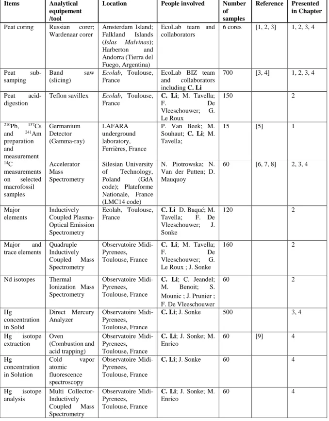
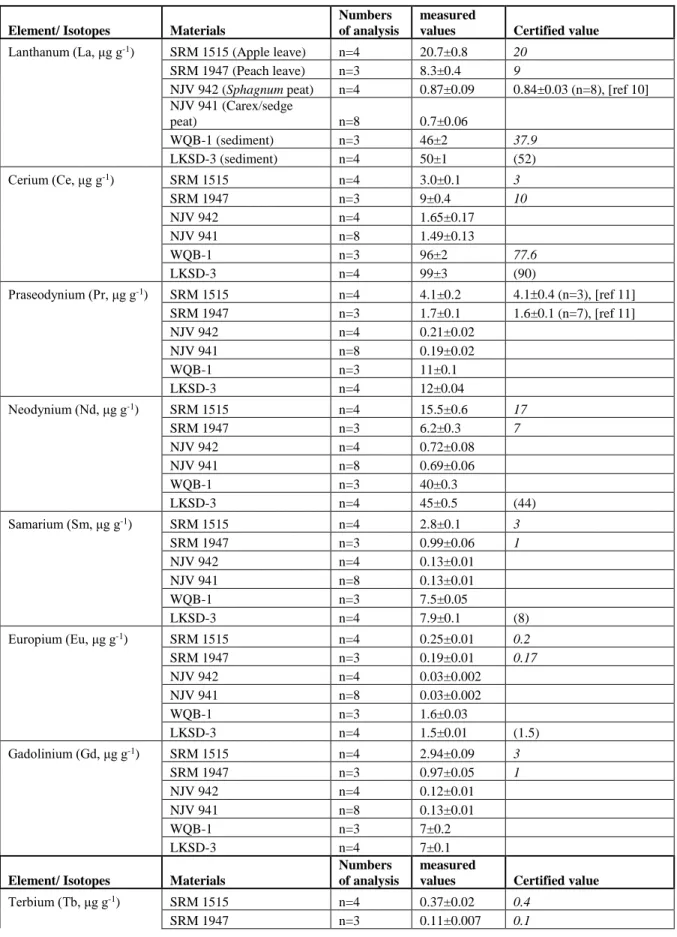
Chapter 1.Recent 210Pb, 137Cs and 241Am accumulation in an ombrotrophic peatland from Amsterdam Island (Southern Indian Ocean) ... 66
Objectifs et résumé ... 67
Research article ... 69
Supporting information ... 91
Chapter 2.Holocene dynamics of the Southern Hemisphere westerly winds over the Indian Ocean inferred from a peat dust deposition record ... 93
Objectifs et résumé ... 94
14
Supporting information ... 135
Chapter 3.Holocene Hg isotope variability in a peat core from the northern edge of Southern Hemisphere westerly winds ... 145
Objectifs et résumé ... 146
Research article ... 148
Supporting formation ... 171
Chapter 4.Unequal anthropogenic enrichment of mercury in Earth’s northern and southern hemispheres ... 172
Objectifs et résumé ... 173
Research article ... 176
Supporting information ... 198
Conclusions and perspectives... 211
1. Peat 210Pb signatures and its function of recent age reconstruction ... 212
2. Atmospheric dust and Hg isotopes: indicators of the Holocene SWW dynamics ... 212
3. Anthropogenic perturbations on atmospheric dust and Hg0 ... 215
4. Perspectives ... 216
15
List of abbreviations
137Cs Cesium isotope with an atom mass of 137 14C Carbon isotope with an atom mass of 14 210Pb Lead isotope with an atom mass of 210 222Rn Radon isotope with an atom mass of 222 241Am Americium isotope with an atom mass of 241
AD Anno Domini
AFS Atomic Fluorescence Spectroscopy
AMS Amsterdam Island
AND Andorra
AUS Australia
BC Before Christ
BP Before Present (1950AD)
CRS Constant Rate of Supply
CV Cold Vapor
DMA Direct Mercury Analyzer
EFalltime Mercury Accumulation Rate Enrichment Factor from Background
periods (pre-1450AD) to 20th century. The periods are defined based on a compilation of global data set.
EFp/b Mercury Accumulation Rate Enrichment Factor from Background
periods (pre-1450AD) to Pre-industrial times (1450-1880AD). The periods are defined based on a compilation of global data set.
EFpreind Mercury Accumulation Rate Enrichment Factor from Pre-industrial
times (1450AD-1880AD) to 20th century. The periods are defined based on a compilation of global data set.
ɛNd Epsilon Neodymium
GEM Gaseous Elemental Mercury (Hg0)
GOM Gaseous oxidized mercury
HAR Harberton
Hg Mercury
16
ICP-OES Inductively Coupled Plasma-Optical Emission Spectrometry
MC-ICPMS Multi Collector-Inductively Coupled Mass Spectrometry
MDF Mass Dependent Fractionation
MIF Mass-Independent Fractionation
NH Northern Hemisphere
PCA Principal Component Analysis
PHg Paticulate-Bound Mercury
PP Primary Productivity
Q-ICPMS Quadruple Inductively Coupled Mass Spectrometry
REE Rare Earth Element
SAF Southern Africa
SCB San Carlos Bog (from the Falkland Islands, Islas Malvinas)
SH Southern Hemisphere
SSA Southern South America
SWW Southern Westerly Winds
17
General introduction
1. Southern Hemisphere atmospheric circulationsMore than ¼ of the CO2 released from anthropogenic activities is absorbed by the global oceans,
which substanstially slows down the rate of climate change (Sabine et al., 2004). The capacity of oceans to absorb CO2 depends on the main processes of sequestration of carbon at the ocean
surface (e.g., diffusion and biological carbon pump) and the subsequent transport from surface to the deep ocean and sediments. Conversely, oceans can also emit CO2 to the atmosphere from
deep ocean by the processes, such as, upwelling and outgassing. The balance between these two sets of processes determines whether oceans act as a net source or sink of CO2. The
Southern Hemisphere (SH) consists of 81% ocean areas, marking the importance of ocean circulation on SH biogeochemistry, ecology and climate. Ocean currents, which convey ocean carbon, are principally driven by atmospheric circulations (Munk and Palmen, 1951). Atmospheric circulations are key control factors of SH climate in the past (Menviel et al., 2018; Saunders et al., 2018), the present (Ogawa and Spengler, 2019) and the future (Swart and Fyfe, 2012; Bell et al., 2019).
One of the main SH atmospheric circulation features is the easterly winds within its corresponding Hadley cell (0-30°S, Hadley, 1735), which controls the spatial distribution of both the tropical rainfall and atmospheric meridional heat transport (Donohoe et al., 2013). The tropical rainfall maximum area, named intertropical convergence zone (ITCZ, Figure 1), lies in the near-equatorial trough and constitutes the ascending branch of the Hadley circulation (Waliser and Gautier, 1993). The ITCZ is formed by the encounter of maritime moist-hot air and continental dry-hot air, leading to high convection, cloudiness and precipitation within the trade wind zone. The ITCZ plays an important role in regulating the atmospheric energy balance by releasing heat during convection and via the planetary albedo by increasing cloud formation (Waliser and Gautier, 1993). The migration and structure of the ITCZ depend on the seasons and the interhemispheric thermal gradient (Donohoe et al., 2013). ITCZ dynamics can affect the shifts in the eddy-driven westerlies and subsequently the global warming in the context of anthropogenic climate change (Ceppi et al., 2013).
18
Figure 1. Positions of
Intertropical Convergence Zone (ITCZ) and Southern Westerly
Winds (SWW) (Toggweiler,
2009).
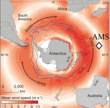
Another important SH climate features is the southern westerly winds (SWW), which prevail between 30 and 60°S with its core belt at ca. 50 - 55°S (Saunders et al., 2018, Figure 2). The position and intensity of SWW vary seasonally due to changes in the sea surface temperature. During the austral winter, SWW shift equatorward and expand, while during the austral summer, SWW move poleward and contract. The SWW dynamics regulate Southern Ocean carbon sink, SH mid-latitude climate, and Southern African, Australian and Southern American aeolian dust trajectories. The displacement of SWW affects the volume of precipitation in SH mid-latitude (e.g., Central Chile, Jenny et al., 2003). SWW are the main driving force of the Antarctica Circumpolar Current - the world’s largest current flowing from the west to the east, connecting the Atlantic, Indian and Pacific oceans. SWW can transport the surface waters to the northern side of the wind belt, leading to upwelling to the south of the wind stress maximum (resurfacing waters from 2-3 km deep) and downwelling to the north (Rintoul, 2010). SWW can also carry dust over long distance from continental sources to remote sites (e.g., Antarctic, Gili et al., 2017).
The Southern Ocean south of 30°S, accounts for approximately 43% of the global oceanic uptake of anthropogenic CO2 over the historical period (Frölicher et al., 2013). By resurfacing
more deep ocean carbon or enhancing more CO2 sequestration at the ocean surface, changes in
the SWW intensity through time are thought to determine whether the Southern Ocean acts as a net source, or sink, of CO2 (Menviel et al., 2018; Landschützer et al., 2015; Hodgson and
Sime, 2010; Toggweiler and Russell, 2008; Thompson and Solomon, 2006; Hodgson, personal communication). This affects atmospheric CO2 concentration and then global climate.
Some models and observations have suggested that the capacity of Southern Ocean to absorb CO2 has weakened under the scenario of increased atmospheric CO2 and strengthened
19
SWW (Le Quéré et al., 2007; Saunders et al., 2018). In this scenario, SWW enhance ocean mixing drawing deep waters with high concentrations of dissolved inorganic carbon to the surface, limiting its capacity to obsorb atmospheric CO2 (Hodgson and Sime, 2010). This
means that Southern Ocean may no longer function as a net sink of CO2. As a result, there
might be a higher level of stabilization of atmospheric CO2 (Le Quéré et al., 2007), which will
enhance global warming. In contast, observations coupled with biogeochemistry models have indicated a strengthened Southern Ocean CO2 sinks since 2002 resulting from an increased
zonal asymmetry in SH atmospheric circulation (Landschützer et al., 2015). Similarly, a model study suggests that poleward-intensified SWW have strengthened the Southern Ocean carbon sink (Russell et al., 2006). Poleward-intensified SWW are suggested to reduce oceanic stratification and allow Southern Ocean to remove anthropogenic CO2 from the atmosphere
(Russell et al., 2006).
Paleoclimate science offers a unique opportunity to investigate the SWW dynamics by providing long-term reconstructions of changes in their strength and position. The reconstructions can be achieved by investigating the wind proxies within different natural archives (ice, sediment and peat) in different SH regions. Numerous archive-based studies have attempted to reconstruct past SWW variability in three different sectors (northern edge with ~35-45°S, core section at ~50-55°S and southern edge below-55°S). The wind variabilities at the northern edge, the core belt and the southern edge of the SWW can be dependent or independent from one another, which highlights the complexity of the SWW dynamics (e.g., Lamy et al., 2001; 2010; Moreno et al., 2010; Lindvall et al., 2011; Van der Putten et al., 2012; Voigt et al., 2015; Saunders et al., 2018). Even though at similar latitude but different longitude, SWW may be recorded with distinct behaviors. For example, during 3-1 cal. kyr BP, Moreno et al., (2010) suggests a poleward-shifted SWW based on pollen signatures from lake sediment at 41°S in Southern Chile, while Voigt et al., (2015) indicates an equatorward-shifted SWW derived from oxygen isotope composition in marine sediment at 38°S in Western South Atlantic. So far, most field studies related to the past SWW dynamics have been conducted in Southern South America (e.g., Lamy et al., 2010; Xia et al., 2018), Southern Africa (e.g., Humphries et al., 2017; Chase et al., 2017) and Australia (e.g., Shulmeister et al., 2004; Marx et al., 2011). By comparison, less attention has been given to SWW records from oceanic islands (e.g., Amsterdam Island, Diego Ramirez Island, Macquarie Island, Saunders et al., 2018), which have minimal continental complex orographic effects and regional climatic effects (e.g., monsoon climate in Australia), and able to directly record SWW variations.
20
Figure 2. Southern Westerly Winds (SWW) and wind speeds. White diamond is the location of Amsterdam Island (AMS), which is the main study site of this PhD. The core SWW belt is between 50-55°S. Arrows show wind direction. (Modified from Saunders et al., 2018)
2. Amsterdam Island peat as an archive of Southern Westerly Winds dynamics
Amsterdam Island (AMS, 55 km2), is located at the northern edge of SWW and halfway between Southern African continent and Australia (Figure 2). This island is sensitive to the changes in the SWW and free from anthropogenic influence. It is an ideal site to study the past SWW variabilities. Ombrotophic peatlands, archives of atmospheric deposition, are widespread in AMS. Details on AMS see the description on “study site” in Chapter 1, 2 and 3.
2.1 Peatlands as archives of atmospheric deposition
A peatland is an ecosystem characterized by organic soils from the accumulation of decomposed plant materials. The organic matter is produced and deposited at a greater rate than it is decomposed, which leads to the formation of peat. Peat net mass accumulation (g m
-2 yr-1) is the balance between annual net primary production and annual decomposition,
regardless of geographic location (Wieder and Lang, 1983). Peat mass is added at the surface and the material will decay after death. The decomposition processes, which cause the collapse of the peat, mainly occur in aerobic conditions (Clymo, 1984) and above the water table. This part of the peat column is referred as the acrotelm (Ingram, 1978). Below the water table, conditions are anaerobic with low oxygen diffusion in water (Clymo, 1984) and this part of the
21
profile is referred as the catotelm (Ingram, 1978). In this section, the decay rate of most materials by anaerobic microflora is much lower than that in aerobic conditions.
Peatlands are estimated to occupy 3.5 million km2, covering 3% of the Earth’s land surface (Gorham, 1991; Lappalainen et al., 1996, Figure 3). More than 85% of the peatlands are distributed in the Northern Hemisphere, under cold temperate climates and high humidity, covering Europe, Russia and North America. Only a small proportion of peatlands (<10%) exists in Southern America, Southern Africa, Australia, New Zealand and small oceanic islands in the Southern Hemisphere (e.g., Amsterdam Island, The Falkland Islands (Islas Malvinas)).
Figure 3. Global Peat Ressources. (Redrawn after Lappalainen 1996).
Peatlands are sensitive to changes in the local hydrological regime and mineral inputs under both climate change and basin geomorphology alternation (e.g., Charman et al., 2009; Mitsch and Gosselink, 2015). Peat cores as environmental archives have the advantages of: 1/ being easy to access due to its worldwide-spread status, especially in the mid-latitudes; 2/ covering Holocene or beyond and 3/ well preserving climatic/atmospheric signals (e.g., macrofossils and chemical elements). Peat cores can be used to reconstruct paleoclimate variability under investigations on multi proxies from biological aspect (e.g., pollen, macrofossils, diatoms and testate amoebae) or from geochemical and isotopic perspectives (e.g., minerogenic input and gas uptake).
22
Ombrotrophic Peatland, one type of peatlands, exclusively receive nutrients, water and pollutants/chemicals from the atmosphere. They are unique to atmospheric deposition study and have been proven to be reliable archives for particle deposition (e.g., dust, Shotyk et al., 2001; De Vleeschouwer et al.,2014; Kylander et al., 2018) and gas deposition (e.g., Hg0, Enrico et al., 2016; 2017).
2.2 Reconstructions of peat chronology
Absolute age constraint plays a fundamental role in reconstructing past climate variability in the environmental archives. Methods by radiocarbon dating (conventional 14C and post-bomb
14C) and 210Pb are widely used in peat studies. Radiocarbon (14C) dating method was discovered
by W.F. Libby, (1949) 70 years ago, which is one of the most reliable dating approaches for the whole Holocene. 14C is the only radioactive form of three natural carbon isotopes (12C, 13C and 14C), with a half-life of 5730 ± 40 years (Godwin, 1962). 14C constitutes of a tiny amount of total carbon, e.g., ~1.2 * 10-10% in the troposphere (Olsson, 1968). 14C is continuously produced in the lower stratosphere and upper troposphere by the interaction of the secondary neutron flux from cosmic ray with atmospheric 14N (Hua, 2009; Gäggeler, 1995). Once
produced, 14C is oxidized to 14CO
2 and subsequently diffuses throughout the Earth Surface.
Terrestrial living organisms can take up CO2 from the atmosphere, with 14C/C ratio similar to
that in the atmosphere. Once the organisms die, they stop exchanging the 14CO2 with
atmosphere. Then 14CO2 decays gradually to 14N. Based on the remaining 14C content and the
decay rate, one can calculate the time (14C age) when the organism died. Peat is mainly formed by organic matters, rich in C content (Charman, 2002). Macrofossils (e.g., Sphagnum, moss) from the peat are generally selected for 14C dating.
210Pb, a natural radioactive isotope of lead, is a decay product of 222Rn. The decay
processes occur in both atmosphere and the soil. The 210Pb faction of atmospheric origin is called “unsupported 210Pb”, which is used to reconstruct the recent age by Constant Rate Supply
(CRS) and Constant Initial Concentration (CIC). CRS model assumes a constant rate of 210Pb supply irrespective of any variations which may have occurred in the sedimentation rate, while CIC model assumes a constant initial 210Pb concentration regardless of any changes in the sedimentation rate (Appleby and Oldfield, 1978). There are many cases that can lead to invalidity in both CRS and CIC models, such as, mixing of the surficial sediment by physical and biological processes (Appleby, 2001), and Pb mobility during the post-depositional stage. In this case, some independent dating proxies are needed to validate the CRS or CIC models. A widely application of chronomarkers are 137Cs and 241Am, which are mainly produced during
23
the nuclear test from 1950s to 1960s with peaking at 1963, and during Chernobyl accident at 1983. Ombrotrophic peatlands receive 210Pb fallout by atmospheric deposition. If CIC model is applicable, the unsupported 210Pb concentration in the peat colume must show a monotonic decline with depth (Appleby and Oldfiled, 1983). Considering the organic decay characteristic of peat, the CIC model may be inappropriate for dating peat accumulations (Appleby and Oldfield, 1992; Appleby et al., 1997). Numerous researches have successfully applied CRS models to the peat archives with validation by chronomarkers (e.g., 137Cs and 241Am, Olid et al., 2013) and/or comparison to post-bomb age (e.g., Davis et al., 2018).
Post-bomb 14C is different from the conventional 14C, with the former of anthropogenic origin and the latter from natural source. Post-bomb calibration curves can be applied to the age reconstruction over the last 70 years (Hua et al., 2013). The tropospheric bomb 14C start to rise in the mid-1950s with peaking in the 1960s due to the influences of aboveground nuclear explosions. At mid to high latitudes, the value of peaked bomb 14C at 1963-1964 almost doubles its pre-bomb level (e.g., Levin et al., 1985). The post-bomb era lasts up to very recent time with a decreasing trend of atmospheric 14C since 1964 (Hua et al., 2013). The decreased atmospheric
14C signature results from the cease of the nuclear detonations and exchange between
hemispheres. The bomb 14C from nuclear test in the atmosphere will die out at ca. 2030 AD
and cannot serve any longer as an age indicator for the periods after 2030.
Age-depth model can be generated with a sequence of 14C dates and/or calibrated calendar ages based on 210Pb or post bomb using classical age modelling (Clam, Blaauw, 2010) or Bayesian methods (Bacon, Blaauw and Christen, 2011). Clam can generate age-depth model in the forms of linear interpolation, linear/polynomial regression and smoothed/cubic splines with calibrated 14C dates (Blauuw, 2010). However, the outliers in the sequence of 14C dates can bias the age model leading to some unrealistic changes in the accumulation rate (Blaauw and Christen, 2005). Bacon is applied to Bayesian statistics and characterized by the assumed constant piecewise accumulation rate. This Bayesian method can be programed with prior knowledge, which allows the researchers adjust the model based on the core conditions. However, the simplified piecewise constant accumulation rate may smooth from a lesser to a greater extent some abrupt change in the deposits. For this case, some additional chronomarkers are needed to better reconstruct the age model, such as, tephra (Vandergoes et al., 2013). Both of Clam and Bacon methods have been widely applied to the global peat study (e.g., Martinez-Cortizas et al., 1999; Marx et al., 2009; Piotrowska et al., 2011; Van der Putten et al., 2015). The choice of methods should be site specific.
24
3. Wind proxies based on the transport and provenance of dust
There are three main groups of wind proxies that used in archive-based studies: 1/ dust provenance and flux (e.g., Vanneste et al., 2015; 2016); 2/ sea salt aerosol flux (directly through geochemical measurements, and indirectly through diatoms and testate amoebae, e.g., Saunders et al., 2018; Whittle et al., 2018); and 3/ rainfall indicators (inferred from macrofossil, pollen, lake levels, magnetic susceptibility, and isotopes, e.g., Van der Putten et al., 2015; Jenny et al., 2003; Lindvall et al., 2011). Below are the introdutions on dust and its potential as wind proxies.
3.1 Atmospheric dust distribution and transport in the Southern Hemisphere
Atmospheric Dust is one type of primary aerosol, while sea salt is another type (Raynaud et al., 2003; Kohfeld and Tegen, 2007). Primary aerosol originates from the dispersal of fine materials from the continental areas (so called dust) and ocean surface (so called sea salt). To be specific, dust is defined as small particles mostly generated by wind from solid materials in the continental regions. Secondary aerosols result from chemical reactions and condensation of atmospheric gases and vapors, e.g., sulfate aerosol droplets formed by oxidation of gaseous dimethylsulfide emitted from marine biogenic activity (Raynaud et al., 2003).
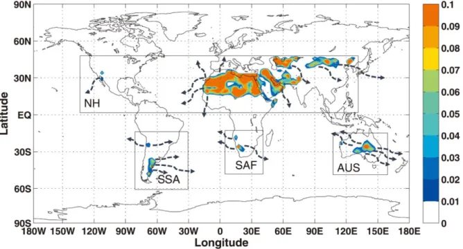
Dust emission and deposition are sporadic phenomena, especially in areas close to the main dust sources (Jickells and Spokes, 2001). There are four main dust source areas on Earth (Bryant et al., 2007; Engelstaedter and Washington, 2007; Prospero et al., 2002; Vickery et al., 2013; Li et al., 2008): (1) Sahara, Arabian and Gobi deserts in the Northern Hemisphere (NH); (2) Kalahari desert in Southern Africa (SAF); (3) Patagonian desert in Southern South America (SSA), and (4) the Great Artesian basin desert in Australia (AUS, Figure 4). Desert dust emissions from most dust sources have doubled over the 20th century due to anthropogenic activities (Mahowald et al., 2010). The current global dust emission is modelled as 2323 Tg yr
-1, with approximately 90% from the NH. AUS shares half of the remaining 10% global dust
emission with 120 ± 8.4 Tg yr-1. SSA plays a second important role in the SH annual dust emission with 50 ± 3.0 Tg yr-1, while SAF contributes 34 ± 2.1 Tg yr-1 (Li et al., 2008). These three SH continents (SSA, SAF and AUS) partially fall in the SWW. SWW can affect the SH dust emissions and depositions by regulating the wind speed and humidity.
25
Figure 4. Global distribution of averaged annual dust emission from 1979 to 1998 (kg m -2 yr-1). The four main dust sources NH, SSA, SAF and AUS represent Northern Hemisphere,
Southern South America. Southern Africa and Australia, respectively. Dark blue dashed arrows represent the main dust trajectories. (Modified from Li et al., 2008)
Atmospheric dust generally goes through three steps in one full cycle: emission, transport and deposition (e.g., Bergametti and Forêt, 2014). Dust generation is a highly complex process that is controlled by multiple environmental factors (e.g., wind, dryness and sparsely-covered vegetation in the soil surface, Mahowald et al., 2005). Dust can be lifted into the atmosphere when high winds pass over the erodible surfaces. When air currents drive the particles along the surface, these particles collide with other solids on the ground, breaking them into smaller pieces, which may easily become airborne and be entrained into the atmosphere (e.g., Van Loon and Duffy, 2017). Wet soil surface and vegetation can stabilize soil dust and limit its mobilization by consuming a proportion of the wind momentum (Mahowald et al., 2005). Thus, an increase in the non-erodible factors can lower the dust availability. Disturbance of the soil surface by anthropogenic activities (e.g., deforestation, agriculture) can facilitate the dust generation, by producing substantial amounts of relatively large particles (tens to hundreds μm diameter) on the soil surface. These large partciles can be “gripped” and transported by the wind (Mahowald et al., 2005). The extra-small particles (i.e., <0.4μm) are not available to wind erosion individually, probably due to agglomeration and adhesive binding with other soil particles (Tegen and Fung, 1994).
26
When being uplifted into the atmosphere, dust can be transported by prevailing winds over hundreds or even thousands of kilometers to remote locations. Saharan dust is carried over long distances and deposits over Europe (Le Roux et al., 2012; Conceição et al., 2018; Gobbi et al., 2019) and the Caribbean Sea (Groß et al., 2016; Velasco-Merino et al., 2018). Dust from the Gobi desert is transported over the Eastern Pacific Ocean (Tan et al., 2017; Dong et al., 2018). Patagonian dust is transported over thousands of kilometers reaching the west coast of South Africa and Australia (Johnson et al., 2011), the Southern Ocean (Neff and Betler, 2015) and East and West Antarctica (Gili et al., 2016; Delmonte et al., 2017). Australian dust is exported to New Zealand (Brahney et al., 2019) and Antarctica (Sudarchikova et al., 2015; Winton et al., 2016).
The loading of atmospheric mineral dust is controlled by dust sources (e.g., aridity, vegetation cover and geology) and climate (e.g., wind strength and airmass circulation) (Harrison et al., 2001; Marx et al., 2018; De Deckker, 2019). For example, higher surface wind speeds can uplift greater amounts of dust. Increased aridity has the potential to expand source areas and decreased atmospheric water content can reduce the washout of sub-micron aeolian dust (Mahowald et al., 2005). The current human-climate interaction (e.g., global warming), can alter dust mobilization by changing the local vegetation cover (Guan et al., 2016; Brahney et al., 2019), and the size of water bodies (Prospero et al., 2002). To study environmental and climatic variability, geochemical dust signatures can be used as wind proxies by assessing dust flux and origins.
3.2 Identification of dust origins
Reconstructions of dust deposition rates and provenances allow us to identify the changes in the source areas and transport pathway associated with climate variability and/or anthropogenic influence (Marx et al., 2018; De Vleeschouwer et al., 2014; Prospero et al., 2002; De Deckker, 2019). Proxies used for source fingerprint range from physical properties (e.g., grain size), to chemical signatures (e.g., rare earth elements), and to isotope compositions (e.g., Neodymium (Nd), Strontium (Sr), Lead (Pb)). Regardless of its nature (physical, chemical and isotopic signatures), dust serving as a tracer should have three characteristics, 1/ representative for a geographical region; 2/ distinctive for that region respect to other areas; 3/ conservative from the source to the sink (Delmonte, 2003).
Different origins of minerals may have different size distributions, which can enable us to distinguish the dust sources in the deposited archives (Stuut et al., 2002; Weltje and Prins, 2007;
27
Gaiero et al., 2013). For example, different dust events have specific fingerprints of particle mode (e.g., a median mode of 12-14 μm, Gaiero et al., 2013). Mineral particles over 20 μm are generally assumed to originate from local/regional areas, because they can rarely be transported over long distances (e.g., several thousands of km) (Lancaster, 2013), except some rare cases (>70μm Saharan dust travelling over 1000km, Betzer et al., 1988). Note that grain size distribution method should be carefully applied to natural archives. For example, in peat studies, a pre-treatment procedure of 550°C for the grain-size analysis, may induce the formation of larger-size salt, which can subsequently bias the results. Conservative chemical elements are less prone to be altered during weathering, transport and the preparation procedures for analysis, which can then well preserve the source information. The conservative properties of the chemical elements coupled with well-developed analytical methods allow us to reconstruct dust flux and identify source origins. The chemical-ratio approaches (e.g., Aluminum/Titanium, Lanthanum/Ytterbium) have been broadly applied to climate-related dust studies in ice cores (e.g., Thompson et al., 2002; Bohleber et al., 2018), sediment (e.g., Bertrand et al., 2014; Frugone-Álvarez et al., 2017; Saunders et al., 2018) and peat (e.g., Shotyk et al., 2001; Marx et al., 2014; Von Scheffer et al., 2019). Since the conservative chemical elements do not always have distinct signatures among different sources, it may be not sufficient to only apply chemical approaches to source identification.
Isotope applications have opened a promising avenue to investigate dust provenance. Isotopic signatures of Nd, Sr and Pb are conservative and may have a distinct geological distribution. For example, 143Nd/144Nd signature (denoted as ɛNd, DePaolo and Wasserburg, 1976) has a range of 15 to 2 in Australia (RevelRolland et al., 2006; De Deckker, 2019), of -25 to -8 in Southern Africa (Grousset et al., 1992; Delmonte et al., 2004; Wegner et al., 2012; Hahn et al., 2016), and of -10 to -3 in Puna-Altiplano Plateau, -6 to 0 in Central Argentina, and of-1 to 5 in Patagonia from Southern South America (Gili et al., 2017). Since targeted isotopes may be less abundant in samples and easily be interfered by other element/isotopes during analysis, isotopic approaches require careful chemical separation from the matrix and highly sensitive mass spectrometry. No dust tracer can be universally applied to every study. Each work should choose the optimum approaches to investigate the dust origin based on the archive itself, lab environment and budgets.
Combining isotope and element geochemistry are effective in identifying the dust sources and subsequently accessing the environmental changes (Kohfeld and Tegen, 2007; Cheng et al., 2018), provided that some conditions are satisfied (e.g., selecting the optimum tracers and
28
easily accessing the the signatures of relevant tracers from the potential source areas). Investigation on dust sources using isotope and elment geochemistry identifies Southern South America (Patagonia and Puna-Altipalno Plateau) as the most important dust source supply to Antarctica (Delmonte et al., 2004; Gili et al., 2017), and to the Atlantic sector of the Southern Ocean during glacial periods (Noble et al., 2012). It is found the supply of continental-sourced detritus to the Southern Ocean during the last glacial period (Noble et al., 2012; Franzese et al., 2006), and an enhanced influence of local Antarctic dust to a peripheral area of the East Antarctic ice sheet during interglacial periods (Baccolo et al., 2018). Isotope and element geochemistry have also been applied to identify the past SWW dynamics in Southern South America (Vanneste et al., 2015; 2016), Southern Africa (Humphries et al., 2017), Australia (Marx et al., 2011) and Macquarie Island (Saunders et al., 2018).
4. Wind proxies based on precipitations using mercury stable isotopes
This section will broadly introduce mercury, its isotopes and its potential as a rainfall proxy.
4.1 Global biogeochemical mercury cycle
The word mercury (Hg) is originally derived from Latin ‘Hydraryrum’ with the meaning of ‘liquid silver’. Compared to silver, Hg, however, can be toxic at low doses in the organic form, methyl-Hg (see section 5, UNEP-GMA, 2018). Hg is the only element which exists in the liquid form at room temperature (melting point, -38.9°C), with a low enthalpy of vaporization (ΔHvap= 59.15 kJ/mol). More than 95% of atmospheric Hg exists as gaseous elemental Hg
(Hg0), while smaller proportions exist as gaseous oxidized Hg (HgII) and particle-bound Hg (PHg) (Shia et al., 1999; Saiz-Lopez et al., 2018). Atmospheric Hg species can transform from one to another under certain conditions. For example, the presence of halogens under sunlight can oxidize emitted-Hg0 into HgII, which finally deposits over the ocean surface in the form of HgII and/or PHg (Vandal et al., 1993; Fu et al., 2016a; Saiz-Lopez et al., 2018). Conversely, HgII can be reduced back to Hg0 by photochemical reactions (Bergquist and Blum, 2007), biotic (Kritee et al., 2007; Demers et al., 2018) and abiotic conditions (Zheng et al., 2018). The speciation of Hg affects its lifespan at the atmosphere, with residence time ranging from days for PHg, to weeks for HgII, and to months for globally-distributed Hg0 (Horowitz et al., 2017; Saiz-Lopez et al., 2018). The long residence time of Hg0 in the troposphere allows it to travel over long distances and deposit to remote areas including Arctic (Korosi et al., 2018), Southern Ocean areas (Angot et al., 2014) and Antarctic (Zaferani et al., 2018).
29
Hg0 is emitted naturally by outgassing of the Earth’s crust and mantle (e.g., volcanism) as primary release, and by re-emission of geogenically-sourced Hg from soil, vegetation and water bodies (e.g., ocean, Amos et al., 2015). In addition to natural release, Hg0 has been substantially liberated from geological depositsby human industrial activities, such as mining, refining and energy production (Pirrone et al., 2010; Streets et al., 2017). When entering the aquatic and/or terrestrial environment, Hg from these two sources will have the same fate for the subsequent life cycle.
Atmospheric Hg deposition over Earth’s surface occurs by vegetation Hg0 uptake (dry deposition, Jiskra et al., 2018), HgII wet and dry deposition (Sprovieri et al., 2017), and Hg0 gas exchange with aqueous water bodies including the Oceans. A growing amount of evidences have highlighted the role of vegetation as Hg0 pump (Obrist et al., 2017; Jiskra et al., 2018; Olson et al., 2019). Vegetation cover constitutes 80% of Earth’s continental surface (Schulze, 1982) and provides substantial leaf surface area for pollutant exchange (Bush and McInerey, 2015). Previous observational studies have shown that leaf interior is the dominant pathway of Hg accumulation under plant growth period (Rutter et al., 2011). Foliar Hg accumulation rate may be species-dependent (Pokharel and Obrist, 2011; Rutter et al., 2011; Teixeira et al., 2018; Pérez-Rodríguez et al., 2018; Olson et al., 2019). Non-vascular vegetation (e.g., peat) accumulates x3 to x6 times more Hg than vascular vegetation (Olson et al., 2019). Hg sequestration by vegetation is controlled by primary productivity, which is related to climate variability (e.g., temperature, humidity, Sala et al., 2018; Wang et al., 2017). Gallego-Sala et al., (2018) suggests longer and warmer growing seasons under global warming will lead to enhanced primary productivity at mid to high latitudes in the future. Increased rainfall can also promote water-limited plant primary productivity (Wang et al., 2017). The influence of climate on plant Hg sequestration can lead to a question: Is it possible to use deposited Hg (e.g., vegetation uptake of Hg0 and input of rainfall HgII) as a proxy to reconstruct the prevailing climate?
4.2 Hg isotope signatures in the environment
Mercury has 7 stable isotopes with a relative mass range of 4% with approximate abundances of: 196Hg (0.16%), 198Hg (10%), 199Hg (17%), 200Hg (23%), 201Hg (13%), 202Hg (30%), 204Hg (6.8%) (Blum and Bergquist, 2007). Hg isotope geochemistry studies have been abundantly conducted since the appearance of high-precision analytical equipment (i.e., Multicollector inductively coupled plasma mass spectrometry). Since Hg stable isotopes have a volatile form (Hg0), redox-active properties and a tendency to form covalent bonds, they can undergo
30
isotopic fractionation (Bergquist and Blum, 2007). Nearly all incomplete, physico-chemical Hg transformations are accompanied by mass-dependent isotope fractionation (MDF, presented by δ202Hg (‰), see equation 1, XXX represents for the mass of isotope). MDF is the
fractionation of isotopes in proportion to the relative difference in the masses. In addition to MDF, Hg isotopes can also undergo mass-independent fractionation (MIF). MIF is the fractionation of isotopes nonlinear to their mass differences. Odd-MIF for odd mass number Hg isotopes is presented by Δ199Hg or Δ201Hg, while even-MIF for even mass number Hg isotopes is presented by Δ200Hg or Δ204Hg (Blum and Berquist, 2007; Young et al., 2002, See equations 2-5). δXXX Hg = {[(XXXHg/198Hg) sample/(XXXHg/198Hg)SRM3133]-1} X 1000 (Eq. 1) Δ199Hg = δ199Hg – (δ202Hg X 0.2520) (Eq. 2) Δ200Hg = δ200Hg – (δ202Hg X 0.5024) (Eq. 3) Δ201Hg = δ201Hg – (δ202Hg X 0.7520) (Eq. 4) Δ204Hg = δ204Hg – (δ202Hg X 1.493) (Eq. 5)
Hg isotope signatures can be used to better constrain on source, transport and transformations of Hg in the environment (e.g., Demers et al., 2018; Sonke, 2011). Two mechanisms relevant to Hg MIF are the magnetic isotope effect (MIE) and the nuclear volume effect (NVE). MIE primarily occurs during photochemical radical pair reactions. Odd-mass isotopes can have high MIF due to its magnetic spin, which can enhance triplet to singlet and singlet to triplet intersystem crossing (Blum, 2012). NVE occurs because nuclear volume and nuclear charge radius do not scale linearly with the number of neutrons. NVE in Hg transformation has not been fully understood. Only a few studies have observed NVE under laboratory environments (Estrade et al., 2009; Zheng and Hintelmann, 2010). Hg isotope mass independent fractionation caused by NVE (< ~0.5 ‰) is found to be smaller than by MIE (> 1‰) (Blum et al., 2014). Hg MIF leads to significant enrichments or depletions of odd mass number Hg isotopes relative to the even ones in environmental Hg pools. Different pathways of Hg transformation can result in different Hg MDF and MIF signatures in the products and reactants. Hg isotopic fractionation can therefore be applied to trace the transformation processes and/or sources. Bergquist and Blum, (2007) found that natural sunlight can lead to photochemical reduction of aqueous Hg species in the presence of organic matter, with a slope of 1.15 ± 0.07 (1σ) in the Δ199Hg/δ202Hg line of produced Hg0 and residual HgII, whereas a
slope of 2.43 ± 0.10 (1σ) in the Δ199Hg/δ202Hg line of produced Hg0 and residual methylmercury under photochemical degradation of methylmercury. After a compilation of Hg
31
isotope study up to 2014, Blum et al., (2014) found different reactions of producing Hg0 from HgII/ methylmercury lead to different Δ199Hg/δ202Hg signatures, with slopes ranging from -3.5 during photochemical reduction from snow (Sherman et al., 2010), to -0.8 during Xenon lamp reduction with thiol ligands (Zheng and Hintelmann, 2010), to 0.1 during equilibrium evaporation, to 1.2 during aqueous photochemical reduction and to 2.4 during aqueous photochemical demethylation. No odd MIF is found during microbial methylation/reduction/demethylation and Thiol-ligand binding/iron oxide in the absence of sunlight sorption (Kritee et al., 2007; 2009; Rodríguez-González et al., 2009).
The development of Hg isotope tools has enabled us to quantify the Hg depositions from different sources. During a long period (> 30 yrs), wet deposition was thought to be dominate Hg deposition over terrestrial environment and great efforts have been given in studying Hg flux in rainfall (e.g., Sorensen et al., 1994; Bullock et al., 2002; Lindberg et al., 2007; Selin et al., 2008; Prestbo and Gay, 2009; Huang et al., 2012; Sprovieri et al., 2017). Relative to wet deposition, Hg dry deposition (e.g., plant uptake of Hg0) is difficult to measure, leading to unclear contributions of Hg dry deposition to the Earth’s surface. Demers et al., (2013) was the first to apply Hg isotopic values (Δ199Hg and δ202Hg) from different sources (foliage,
underlying mineral soil and rainfall) to reconstruct the Hg sources in forest floor. The authors found that only ~16% of input is from rainfall, which is against the dominant role of Hg wet deposition. The authors attribute the lower Hg wet deposition to a greater throughfall input, assuming that the isotopically unconstrained throughfall has similar Hg isotopic signatures as foliage. Similarly, some other studies also suggest a dominant Hg dry deposition to the boreal forest floor, rather than HgII precipitation, by Hg isotope MIF and/or MDF mixing calculation (Jiskra et al., 2015; Zheng et al., 2016; Wang et al., 2017). These studies have broadly distinguished the contributions of Hg dry and wet deposition, even though their approach of using Δ199Hg and/or δ202Hg is not free from bias. MDF (δ202Hg) can fractionate during the
source mixing (e.g., preferential of light isotope uptake by plant) and Hg transformation, while MIF (Δ199Hg) can occur under photochemical reduction. Overall, δ202Hg and Δ199Hg might
have given unprecise output in source mass balance calculation.
4.3 The potential of Hg stable isotopes as rainfall proxies
MIF of even Hg isotopes (reported as Δ200Hg and Δ204Hg) is thought to be conservative at the Earth’s surface. Even MIF isn’t observed in anthropogenic Hg sources, but it is present in precipitation (Gratz et al., 2010; Chen et al., 2012; Demers et al., 2013; Enrico et al., 2016; Obrist et al., 2017) and in ambient atmospheric Hg0 (Enrico et al., 2016). In general, Hg0 is