HAL Id: tel-00701545
https://tel.archives-ouvertes.fr/tel-00701545
Submitted on 25 May 2012
HAL is a multi-disciplinary open access
archive for the deposit and dissemination of sci-entific research documents, whether they are pub-lished or not. The documents may come from teaching and research institutions in France or abroad, or from public or private research centers.
L’archive ouverte pluridisciplinaire HAL, est destinée au dépôt et à la diffusion de documents scientifiques de niveau recherche, publiés ou non, émanant des établissements d’enseignement et de recherche français ou étrangers, des laboratoires publics ou privés.
Feature selection based segmentation of multi-source
images : application to brain tumor segmentation in
multi-sequence MRI
Nan Zhang
To cite this version:
Nan Zhang. Feature selection based segmentation of multi-source images : application to brain tumor segmentation in multi-sequence MRI. Other. INSA de Lyon, 2011. English. �NNT : 2011ISAL0079�. �tel-00701545�
Numéro d’ordre: 2011-ISAL-0079 Année 2011
THÈSE
présentée devant
L’Institut National des Sciences Appliquées de Lyon
pour obtenir
LE GRADE DE DOCTEUR
ÉCOLE DOCTORALE: ÉLECTRONIQUE, ÉLECTROTECHNIQUE, AUTOMATIQUE
FORMATION DOCTORALE : SCIENCES DE L’INFORMATION, DES DISPOSITIFS ET
DES SYSTÈMES
par
ZHANG Nan
Feature Selection based Segmentation of Multi-Source Images:
Application to Brain Tumor Segmentation
in Multi-Sequence MRI
Soutenue le 12 septembre 2011 Jury :
Yue-Min ZHU Directeur de recherche CNRS Co-Directeur de thèse
Su RUAN Professeur Co-Directeur de thèse
Qing-Min LIAO Professeur Co-Directeur de thèse
Pierre BEAUSEROY Professeur Rapporteur
Da-Tian YE Professeur Rapporteur
SIGLE ECOLE DOCTORALE NOM ET COORDONNEES DU RESPONSABLE
CHIMIE
CHIMIE DE LYON
http://sakura.cpe.fr/ED206 M. Jean Marc LANCELIN
Insa : R. GOURDON
M. Jean Marc LANCELIN
Université Claude Bernard Lyon 1 Bât CPE 43 bd du 11 novembre 1918 69622 VILLEURBANNE Cedex Tél : 04.72.43 13 95 Fax : [email protected] E.E.A. ELECTRONIQUE, ELECTROTECHNIQUE, AUTOMATIQUE http://www.insa-lyon.fr/eea M. Alain NICOLAS Insa : C. PLOSSU [email protected] Secrétariat : M. LABOUNE AM. 64.43 – Fax : 64.54 M. Alain NICOLAS
Ecole Centrale de Lyon Bâtiment H9
36 avenue Guy de Collongue 69134 ECULLY Tél : 04.72.18 60 97 Fax : 04 78 43 37 17 [email protected] Secrétariat : M.C. HAVGOUDOUKIAN E2M2 EVOLUTION, ECOSYSTEME, MICROBIOLOGIE, MODELISATION http://biomserv.univ-lyon1.fr/E 2M2 M. Jean-Pierre FLANDROIS Insa : H. CHARLES M. Jean-Pierre FLANDROIS CNRS UMR 5558
Université Claude Bernard Lyon 1 Bât G. Mendel 43 bd du 11 novembre 1918 69622 VILLEURBANNE Cédex Tél : 04.26 23 59 50 Fax 04 26 23 59 49 06 07 53 89 13 [email protected] EDISS INTERDISCIPLINAIRE SCIENCES-SANTE
Sec : Safia Boudjema
M. Didier REVEL
Insa : M. LAGARDE
M. Didier REVEL
Hôpital Cardiologique de Lyon Bâtiment Central
28 Avenue Doyen Lépine 69500 BRON Tél : 04.72.68 49 09 Fax :04 72 35 49 16 [email protected] INFOMA THS INFORMATIQUE ET MATHEMATIQUES http://infomaths.univ-lyon1.fr M. Alain MILLE M. Alain MILLE
Université Claude Bernard Lyon 1 LIRIS - INFOMATHS Bâtiment Nautibus 43 bd du 11 novembre 1918 69622 VILLEURBANNE Cedex Tél : 04.72. 44 82 94 Fax 04 72 43 13 10 [email protected] - [email protected]
Matériau x
M. Jean Marc PELLETIER
Secrétariat : C. BERNAVON 83.85
INSA de Lyon MATEIS
Bâtiment Blaise Pascal 7 avenue Jean Capelle 69621 VILLEURBANNE Cédex
Tél : 04.72.43 83 18 Fax 04 72 43 85 28 [email protected]
MEGA
MECANIQUE, ENERGETIQUE, GENIE CIVIL, ACOUSTIQUE
M. Jean Louis GUYADER
Secrétariat : M. LABOUNE PM : 71.70 –Fax : 87.12
M. Jean Louis GUYADER
INSA de Lyon
Laboratoire de Vibrations et Acoustique Bâtiment Antoine de Saint Exupéry 25 bis avenue Jean Capelle 69621 VILLEURBANNE Cedex Tél :04.72.18.71.70 Fax : 04 72 43 72 37 [email protected] ScSo ScSo* M. OBADIA Lionel
Insa : J.Y. TOUSSAINT
M. OBADIA Lionel Université Lyon 2 86 rue Pasteur 69365 LYON Cedex 07 Tél : 04.78.77.23.88 Fax : 04.37.28.04.48 [email protected]
Abstract
Magnetic Resonance Imaging (MRI) is widely applied to the examination and assistant diagnosis of brain tumors owing to its advantages of high resolution to soft tissues and none of radioactive damages to human bodies. Integrated with medical knowledge and clinical experience of themselves, the experienced doctors can obtain the sizes, locations, shapes and other pathological characteristics of brain tumors according to the information in MRI images to make scientific and reasonable therapeutic treatment.
Because there are several MRI examinations for every patient in the whole therapeutic treatment, each of which can give 3-dimensional data in multiple sequences, it is a large amount of data to be dealt with for the doctors. Long time of hard work will inevitably lead to mistakes in the diagnosis of the tumor contours for the doctors. Moreover, it is subjective for the doctors to determine the state of the diseases according to their medical knowledge and clinical experiences. Therefore, developing an automatic or a semi-automatic computer-aided diagnosis system is meaningful in real medical treatments, which can release the workload of doctors and improve the accuracy by giving objective results.
This problem is a hot point in the research field of biomedical engineering and a lot of algorithms have been proposed to try to solve it. But unfortunately it is still unsolved due to the limitations of low accuracy, efficiency, applicability and robustness of existing algorithms. In this thesis, a semi-automatic brain tumor detection and classification framework from tumor region segmentation to tissue classification is proposed with Support Vector Machine (SVM) as its classifier. Through fusion of input data, extraction of feature vectors, feature selection, primary classification of brain tumor and contour refinement, the final tumor detection and classification can be fulfilled. Multi-kernel SVM is also introduced in our proposed system to be fit to multiple MRI sequences and to improve segmentation accuracy. In addition to the multi-kernel SVM, adaptive training is designed to follow-up the changes of tumors during several MRI
examinations. By adaptive training, the system can obtain the properties of tumors after the first detection and classification and then separate the tumors in the subsequent MRI examinations automatically.
The proposed system is evaluated on 13 patients with 24 examinations, including 72 MRI sequences and 1728 images. Compared with the manual traces of doctors as the ground truth, the average classification accuracy reaches 98.9%. The system utilizes several novel feature selection methods to test the integration of feature selection and SVM classifiers. Also compared with the traditional SVM, the neural network and a level set method, the segmentation results and quantitative data analysis demonstrate the effectiveness of our proposed system.
Key words: brain tumor detection; Support Vector Machine (SVM); feature
Table of Content
1.1 Background ... 8
1.2 Magnetic Resonance Imaging Theory ... 10
1.3 Related Works ... 15
1.3.1 Basic Image Processing Methods ... 15
1.3.2 Basic Pattern Recognition Methods ... 17
1.3.3 Fuzzy Theory-based Method ... 18
1.3.4 Deformable Model-based Method ... 20
1.3.5 Tumor Detection in Multiple MRI sequences ... 21
1.4 Work of This Paper ... 23
2.1 Feature Selection Theory ... 25
2.2 Feature Selection Algorithms ... 27
2.3 Summary ... 38
CHAPTER 3 TUMOR DETECTION IN MRI IMAGES ... 39
3.1 The Framework of the Proposed System ... 39
3.2 SVM-based Classification Subsystem ... 42
3.3 Region Growing-based Contour Refinement Subsystem ... 49
3.4 Adaptive Training-based Tracking Subsystem ... 50
3.5 Summary ... 52
CHAPTER 4 EXPERIMENTATION AND DISCUSSION ... 53
4.1 Experimental Data ... 53
4.2 Experimental Results ... 55
4.3 Comparison and Analysis of Feature Selection Methods ... 61
4.4 Selection of Some Key Parameters ... 66
4.5 Effectiveness of Features ... 68
4.6 Discussion and Evaluation of Contour Refinement ... 77
4.7 Effectiveness of Adaptive Training ... 80
4.8 Comparison with Other Methods ... 84
4.9 Tissure Classification ... 91
CHAPTER 5 CONCLUSION ... 95
5.1 Conclusion of Contributions ... 95
5.2 Future Work ... 96
Publications de l’auteur ... 98
CHAPTER 1 INTRODUCTION
1.1 Background
With the growing extent of aging population, cancer has become a global public health problem. According to the World Cancer Research Fund’s latest statistics, cancer is the world’s first cause of death. In the worldwide each year, 12.7 million people are diagnosed with cancer, and 7.6 million people died of cancer [1]. Meanwhile, the annual incidence of cancer continues to rise. By 2030, every year there will be 26 million new cases, and the death toll will reach to 1.7 million people.
As a kind of cancer, brain tumor is a very malignant and harmful disease. It has a high incidence, and high mortality, which ranks the fifth in the whole tumors and is just below the stomach cancer, uterine cancer, breast cancer and esophageal cancer [2-3]. Diagnosis and treatment of brain tumor cost a longer period, usually one examination every a few months. The doctors need to check on the stage of the disease in last examination as referral, and to develop the treatment plan for the next therapy. Under the existing medical conditions, in addition to surgery and radiation therapeutic methods, there are no more effective treatments, and the patients’ condition can be alleviated and controlled, but extremely difficult to cure, which will cause great burdens in both mentality and economy for the patients [4-5]. In this sense, the treatment of cancer is a major social problem in both economic and financial aspects. A good solution to this problem will have important social and practical significance.
For early detection and treatment of brain tumors, some medical image-based diagnosis methods are widely applied to clinical practice. Through a variety of medical imaging, the doctors can obtain and understand the patient’s condition more clearly and intuitively, and propose various types of scientific and rational treatment plannings for the patients.
Commonly used medical imaging methods are Computed Tomography (CT), Positron Emission Tomography (PET), CT / PET, Magnetic Resonance Imaging (MRI), and so on [6].
CT uses the radioactive rays to penetrate the human body, and the imaging is based on the different characteristics reflecting to the rays of different tissues. PET needs to inject with radioactive drugs in the human body, and the drugs will flow to all the cells, tissues and organs with the blood in the whole body. The absorbed radiation will be metabolized and released by different tissues to form different rays which can be received for a specific imaging. CT/PET refers to the combination of CT and PET scans which are carried out on the same plane to form a fused image with the machine. Both CT and PET examination have radioactive hazards, and PET examinations are too expensive. Compared with all these imaging modalities above, MRI is the most cost-effective [7].
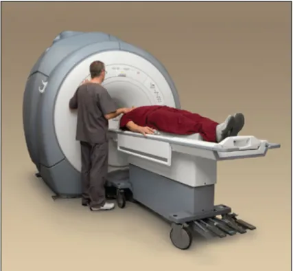
The schematic diagram of MRI equipment and inspection is shown in Figure 1.1 [8].
Figure 1.1 The schematic diagram of MRI equipment and inspection.
In the MRI imaging process there will be not any instruments entering and any medication injected into the human body. There is not any radiation damage to the human body, and the whole process is quite safe. In addition, MRI imaging has high-resolution and accurate positioning of soft tissues, and is sensitive to the characteristics of diseases, thus it is especially suitable for the diagnosis of brain diseases [2, 9].
After obtaining the MRI images, in radiotherapy or surgery situations, the doctors need to clearly grasp the patient’s condition according to the relevant images and to fully prepare for the disease treatment based on the medical information. General speaking, according to the obtained MRI images and their clinic knowledges and experiences, physicians can fulfill the manual segmentation of images to reasonably grasp the size, shape, location, structure distribution and other lesions of the tumor regions [10].
However, under the existing medical conditions, all of the above work can only be done manually by the doctors themselves. On one hand, this is undoubtedly a great burden for the doctors to work on a large number of MRI examination data from many patients. Doctors’ hard work will inevitably make errors in the classification results. On the other hand, the manual segmentation results are very subjective, that is to say, different doctors may lead to significantly different segmentation results, and the segmentation results from the same doctor but at different moments may be also
different, which undoubtedly brings a certain degree of risk to the diagnosis of the patients.
There are mainly two common types of brain tumors, meningiomas and gliomas. The characteristics of meningioma are relatively simple on the medical images, in which there is a clear distinction border between normal tissues and tumors. So meningiomas is easy to be segmented and removed directly through the surgical operations. The characteristics of gliomas are invasive, that is, tumors and other abnormal tissues will be invasive and spread into normal tissues to some degree, and all the tissues are close mixed together, so it is very difficult to clearly distinguish them manually by the doctors. Common practice in real clinical surgery is to appropriately excise the determined tumor tissues through the operation, and then to extract the remaining tissues and cells near the cut boundary to accomplish the pathological analysis in order to test the components and the proportion of cancer cells, which determines the surgical excision extent of the abnormal tissues and the treatment program of the next step [8-10].
The detection and segmentation of brain tumors are of great significance, and also there are problems and risks in the process. In this paper will research on the detection and analysis of the complex glioma and present a semi-automatic segmentation and detection system on brain tumors as to the difficulties in the current computer-aided analysis means. The framework can decrease the degree of interaction from human bodies, reduce the workload of doctors, establish a sound mechanism for medical image processing using medical knowledge, and provide a relatively accurate results which can be accepted by most physicians as objective references to assist doctors to diagnose and treat disease. Meanwhile, the system can adaptively track the patient’s condition effectively to assess the scientificalness and rationality of the treatment. If a large number of clinical data can be used for statistical analysis and experimental validation, the system also has practical significance.
1.2 Magnetic Resonance Imaging Theory
Nucleus in the tissues of human body is composed of protons and neutrons. Protons have a positive charge, and neutrons are not charged, thus the whole nucleus is shown as positively charged. Charged nucleus rotates around its own axis rapidly, and from the law of electromagnetic induction, high-speed spin will produce a vertical magnetic moment. According to the different natures of spin, the nuclei can be divided into two different types: magnetic nuclei and nonmagnetic nuclei. The former denotes the nuclei which can generate a magnetic moment by the spin, and the latter denotes those which can not generate a magnetic moment. If the numbers of protons or neutrons in a nucleus is odd, then the nucleus belongs to the magnetic nuclei; otherwise the nucleus is non-magnetic nuclei if and only if the numbers of protons and neutrons inside an atomic nucleus are both even. Only the magnetic nuclei can be used for the magnetic
resonance imaging [11].
In theory, the magnetic neclei of all elements can be used for MRI imaging, but in the current imaging mode, only hydrogen nuclei just with one neutron proton (not the other isotope of hydrogen atoms) are mainly used. This is mainly due to [12]:
1. in the body hydrogen atom has the highest molar concentration: the human body contains a lot of water and hydrocarbons (such as sugar, protein and fat, etc), so the amount of hydrogen nuclei in the human body is the highest, more than 2/3 of the total human nuclei. Sufficient hydrogen nuclei will be very beneficial in generating a strong magnetic resonance imaging signal, and the actual magnetic resonance imaging also mainly relies on hydrogen nuclei in the water and fat.
2. hydrogen nuclei has the maximal susceptibility: compared with the nuclei of other elements in the human body, the susceptibility of the hydrogen nuclei is on the highest level. Higher degree of magnetization will generate higher signal intensity in the magnetic resonance imaging.
3. the biological characteristics of hydrogen nuclei are obvious: because there are a lot of water and hydrocarbons in the body, hydrogen nuclei exist in the various tissues of the body. Using hydrogen nuclei for magnetic resonance imaging can describe the different characteristics of a variety of different tissues in the human body with images and thus hydrogen nuclei can lead to a strong biological representation.
The typical MRI imaging system mainly consists of five parts: the main magnet, gradient systems, RF system, computer systems and other auxiliary equipment [11], as shown in Figure 1.2 [13].
Figure 1.2 Structure of MRI imaging System
The main magnet is a device to produce a magnetic field, and its performance will directly affect the imaging quality of MRI. Generally speaking, the main magnet can be divided into two defferent types: permanent magnet (made of permanent magnet
Gradient System Main Magnet RF System Control Panel Computer Preamplifier Gradient Coil Gradient Amplifier RF Amplifier RF Transmitting Coil RF Receiving Coils Auxiliary Equipment
material) and electromagnetic magnet (twined by coils). Gradient system is used to generate the linear gradient magnetic field, to code the spatial orientation of MRI signal and the switch of gradient field will generate the MR echo. RF system mainly consists of Radio Frequency coils which are used to receive the generated MR echo. Computer system controls the entire operations of the MRI imaging system, including pulse excitation, signal acquisition, data operations and image display. Supplemented by some multi-function softwares, computer system can obtain other complex capabilities, such as data mining and analysis, three-dimensional modeling and so on. Auxiliary system mainly refers to the auxiliary equipments that ensure the normal operation of the MRI imaging system [11].
The detailed imaging process of MRI can be described as:
After the human body enters the main magnetic field, it can produce magnetization phenomena: the magnetic moments from the spin of hydrogen nuclei themselves will deflect along the orientation of main magnetic field. Most magnetic moments will be forward the direction of the magnetic field and into a low-level energy state, and a small number of hydrogen nuclei will be against the direction of the magnetic field and remain high-level energy state. The total magnetic moment vector (called the longitudinal macro-magnetic moment) maintains the same direction with the main magnetic field.
Macro-magnetic moments of different tissues are concerned with the number of hydrogen nuclei in tissues. The higher the content of hydrogen nuclei is, the stronger the longitudinal macro-magnetic moment will be produced. However, the level of macro-magnetic moment vector is still much smaller than that of the main magnetic field, and both of them are in the same direction. Superimposed with each other, the macro-magnetic moment vector will be completely submerged in the main magnetic field. The strength of the pulse signal released from the longitudinal magnetic moment is too weak to be received by the RF coil. Thus it is not feasible to distinguish different tissues according to different levels of macro vectors caused by differnet amount of hydrogen nuclei.
In order to distinguish different tissues, RF pulses are applied by the imaging system to the human body in the main magnetic field. The energy of pulses will be delivered to the hydrogen nuclei in a low energy level to make them achieve the transition to the high energy level by energy absorption. This phenomenon is the so called magnetic resonance phenomenon. The macro-magnetic moment vector deflects under the input pulses. The stronger the energy of RF pulse is, the greater the angle of deflection is. After the absorption, the energy of hydrogen nuclei is in a high and unstable level. Once the RF pulse is removed, the energy will be released automatically and the hydrogen nuclei will return to the initial steady state. In the recovery process, electromagnetic pulses will be released and received by the RF coil for imaging.
The recovery process of macro-magnetic moment vector after the disappearance of pulses is also called the relaxation process, which is divided into two types, namely,
lateral relaxation (transverse magnetization component decreases to disappearance) and longitudinal relaxation (longitudinal magnetization component increases gradually back to the initial value). Both of the relaxation correspond to T2 and T1 characteristics of the tissues respectively. Different tissues have a significant difference in characteristics of T2 and T1 [11-12].
Given different excitation pulse sequences, MRI can form different weighted sequences to reflect the different characteristics and biological properties of tissues. Commonly used MRI sequences are T1-weighted, T2-weighted, PD-weighted (Proton Density) and FLAIR (FLuid Attenuated Inversion Recovery) weighted sequences. T1-weighted images reflect the ability about the recovery speed of magnetic moment in the longitudinal relaxation, while T2-weighted images reflect the decay speed of magnetic moment in the transverse relaxation. PD-weighted images reflect the differences among protons (hydrogen nuclei) density (content per unit volume). After the suppression of free water in the T2 weighted images to get better display of the tumor characteristics, FLAIR-weighted images can be obtained [11-12].
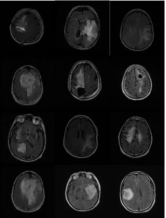
Examples of T1-weighted, T2 weighted and FLAIR-weighted images of the same patient in a same imaging process are shown in Figure 1.3 [2].
Figure 1.3 Examples of MRI weighted images
(from left to right: T1-weighted, T2 weighted and FLAIR-weighted images)
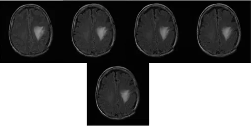
MRI imaging sequences are composed of multiple slices, of which the positions and thickness can be chosen randomly, as shown in Figure 1.4 [14]. The red, blue and green rectangles refer to commonly used imaging directions to the MRI slices. Different weighted image sequences contain a different number of slices. Generally speaking, T1-weighted sequence contains the most slices (usually 124 slices), while T2 weighted, PD-weighted and FLAIR-weighted sequences usually contain the same number of images as 24.
Brain tissues in MRI images can always be divided into two main types: normal tissues, including gray matter, white matter and cerebrospinal fluid (CSF), and abnormal tissues, usually containing tumor, necrosis, cystic degeneration and edema. Necrosis is in the tumor region in general, while generally cystic change and edema are located near the tumor border. These two types of tissues often overlap with the normal tissues and
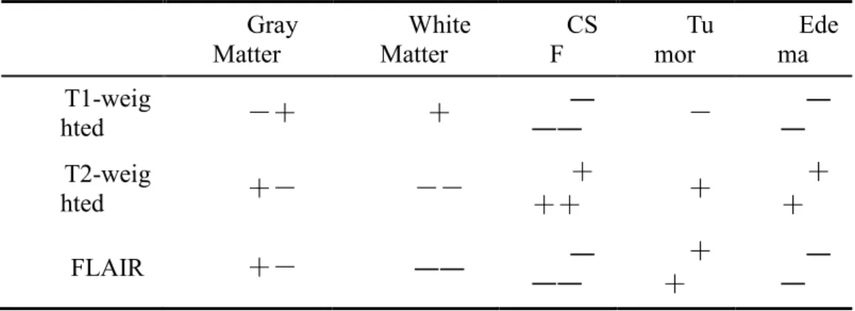
they are not easily to be distinguished. The gray contrast of major tissues in different MRI sequences is shown in Table 1.1 [2].
Figure 1.4 The selection directions of MRI slices
Table 1.1 The gray distribution of different tissues in multiple MRI sequences
Gray
Matter Matter White F CS mor Tu ma Ede
T1-weig hted -+ + ―― ― - ― ― T2-weig hted +- -- + ++ + + + FLAIR +- ―― ― ―― + + ― ―
In Table 1.1, the negative sign denotes the low gray value, and the positive sign denotes the high gray value. The larger the number of negative signs is, the darker the relevant region is. The corresponding region is much lighter while the number of the positive sign is larger. It should be noted that Table 1.1 can just indicate the gray value contrast in the internal tissues of the same weighted sequence, and different MRI sequences can not be comparable due to the different imaging parameters, imaging environment, imaging equipment and the patient’s specific case. In addition, the tumor area typically includes a variety of abnormal tissues, so its intensity distribution will be uneven, which can also be used as one of the prerequisites for the classification of the internal tissues of the tumor region [2].
1.3 Related Works
MRI images can reflect details of different features to provide an important basis for the diagnosis and treatment of illness for patients. However, there are still some restrictions in computer-based analysis of MRI medical images, such as: the differences of imaging equipment, imaging environment and imaging parameters among patients; the redundancy, noise and other interference factors inevitably from the formation of the images; the large amount of image data from multiple sequences to be dealt with; the uniform patients’s conditions among large individuals; the lack of available priori knowledge; the complex structure of MRI images, including different tissues in the internal and external region of the tumors; and the lack of clarity aliasing of the tumor borders due to the the invasive characteristics of gliomas.
The variety of restriction above limit the degree of automation in a MRI-based medical image processing systems, that is to say, to develop an accurate and efficient fully automatic system is almost impossible. The issue is also a hot and difficult problem in the international interdisciplinary fields of medicine and information, and it has been active in the forefront of research. A lot of work around this issue are carried out, and a variety of innovative or improved methods are conducted to try to solve this problem.
At present a successful method is to develop a semi-automatic system with the combination of human interaction, which can improve the automatic level of the system on one hand, and reduce the excessive interaction involved on the other hand. Through the auxiliary means (pre-or post-processing steps) the system can take full advantages of multi-modality MRI sequence data and directly optimize the classifiers to improve classification accuracy and efficiency.
1.3.1 Basic Image Processing Methods
The traditional analysis on MRI images can ignore the medical information implied in the images, and deal with them directly as a general image processing problem to operate. Corresponding to each two-dimensional MRI slice, using some image processing methods to grasp regions with the same or similar characteristics to achieve the separation. Regions with coherent characteristics are not necessarily consecutive, and there may be the case where the region is composed of blocks. And other regions of different characteristics are distinguished from other parts to complete the preliminary analysis of the two-dimensional slice. It can be observed that, the traditional tumor detection in MRI images is a typical image analysis problem.
A variety of traditional image processing algorithms can be applied to try to resolve this problem. The most common algorithm is the threshold-based method [15], which is always integrated with histogram analysis [16] to first obtain the overall histogram distribution of the image, then to select the appropriate threshold based on the distribution of the binary image, and finally to finish segmenting the image area
supplemented post-processing processings of morphological operations [16], such as hole filling, boundary improvement, and so on. However, this method is too simple. If the histogram of the image does not contain obvious peaks or valleys, it will be difficult to select the optimal threshold. A commonly automatic threshold selection method is called Otsu Threshold [17], but its accuracy can not still reach a higher level, that is because the algorithm itself is too simple and can not be adaptive to the complex situations of images.
Considering the characteristics of the the whole tumor area, such as the similarity, uniformity or gradual change among the gray levels, region segmentation methods can be used to achieve the detection of tumors. Commonly used algorithms are region growing algorithm and regional separation and merger algorithm [18] .
Region growing algorithm requires a certain amount of pre-selected seed points, then the growth area is expanded by determining the similarity of the gray values of the pixels within the scope of the seed points, and ultimately achieves the purpose of image segmentation. Algorithm is limited by the stopping criteria. In general, if the criterion does not meet the conditions of similarity, the algorithm will automatically stop. But in MRI images, the characteristics of the tumor borders and normal tissues are closely similar, which leads to the situation that the similarity condition of neighborhood and the seed points can always be satisfied. Therefore, it is generally necessary to manually set more stringent criteria to make the algorithm stop.
Regional separation and merger algorithm extends the seed points to the seed regions and the segmentation algorithm is just the opposite with the region growing processing. First, the initial image is randomly divided into a number of non-overlapping regions, then these areas will continue to be divided into much minor parts more detailedly, and finally these similar parts are merged together in accordance with the very close similarity criterion. Because the image has been precisely refined to the small extent, the characteristics of the adjacent pixels and regions are much closer to each other, and the merger operation will be more accurate and simple. But the algorithm does not limit the detailed extent of the image segmentation, and the merger guidelines are also required artificial selection, all of which will influence the algorithm’s performance to a certain extent.
Altas-based segmentation methods, also called registration-based methods, utilize the same area characteristics of the images. The normal human brain tissue indicates a symmetric structure, therefore the algorithm pre-create multiple templates to construct a template library. The image needed segmenting will be registered to the templates one by one through different linear, non-linear or combination maps to establish the corresponding relationship between the segmented image and the templates, so as to achieve the purpose of segmentation and classification [19-22]. Registration-based method is more suitable for segmentation of normal brain tissues, but because of the need to establish templates in advance, the algorithm is sensitive to the initial templates, the accuracy of which will influence the segmentation accuracy to a great extent. That is
the limitation of this type of algorithms.
Regional algorithms use the approximate characteristics (similarity) between adjacent pixels, and oppositely the corresponding boundary algorithms use the properties of huge differences around the boundary pixels, such as the jumping intensity, complex contour, gray gradient, the level of the frequency spectrum, and so on. Commonly used boundary detection algorithms are based on a variety of edge detection operators [16], such as the Canny operator, Sobel operator and so on. These operators are equal to discrete square templates with variable sizes of 3 3× , 5 5× , etc. The
templates move pixel by pixel in the entire image, and the combination of the central pixels of the templates which correspond to the convolution result is the relevant border. Edge detection always obtains discrete contour points, and we must utilize a variety of connectivity techniques to get a complete outline of the border. Various edge detection operators have their advantages and disadvantages themselves, but all of them are generally sensitive to noise and slightly lack of accuracy.
1.3.2 Basic Pattern Recognition Methods
The basic elements of MRI images are the pixels, and each pixel contains a variety of features about image properties, including the basic gray-scale [23], a variety of features derived from the characteristics of the basic features, such as texture features (including mean value, standard deviation, and the commonly used Gray Level Concurrence Matrix (GLCM) to reflect statistical characteristics [24-25], and so on), mathematical transformation features (such as wavelet transform features [26-28]) and so on. Various features are related to the corresponding meaningful information in the relevant field, which can indicate a specific physical meaning through certain numerical values and its scope of change. Pattern recognition algorithms research on the pixels and include features as the study objectives. By analyzing and comparing different characteristics, the corresponding pixels are classified into different categories.
Commonly used pattern recognition algorithms are clustering, Bayesian probability model, linear and nonlinear discriminant classification methods [29]. Clustering mainly uses the gray values of the image, and merges data points of different types according to the clustering criteria based on similarity. A typical unsupervised clustering algorithm is the nearest neighbor method, in which the data is clustered into the same category as that of the nearest point. The improved algorithms are K-nearest neighbor (KNN) method (the data is clustered into the same category as that of the K nearest points), edited nearest neighbor (nearest neighbor method becomes to a two-step process: the first step is the pre-classification of data to remove the misclassification data, and the next step is to classify using the KNN criterion to improve accuracy), and so on. Nearest neighbor method is relatively simple: one point is just compared with another data point in classification. The algorithm is not reliable enough and can not handle the situation of complex boundary, or of points very far from the center of the class when the distribution of the elements is long and narrow, the same as some types of its improved
algorithms.
Another commonly used clustering algorithm is C-means clustering (C-means), in which all the centers of the classes are prefixed in advance. During classification, the distances between each data point and all the centers are computed, and the data is classified using the nearset distance criterion. Class centers will automatically be updated as the change of the classification of data sets and its containing elements. The limitations of C-means clustering is that the number of classes needs to be pre-set and can not be changed in the clustering process. This algorithm is relatively simple and can not handle the situation of the existence of outliers (data is very far from the center of this class and is wrong classified). The improved algorithms of C-means clustering, such as ISODATA, have also been widely applied [29].
Bayesian probability model-based classification is to cluster data points into the corresponding categories by calculating the posterior probability of data points, and decision criterion used is always the minimal risk criterion. This algorithm can be easily extended to the case of multi-dimensional data and multi-class classification, but the number of data sets and the probability distribution of all the elements are needed to be known in advance, otherwise it is impossible to calculate the probability.
Linear discriminant algorithms mainly refer to that the classification surface is a plane or a hyperplane, which can be described using the linear equations. Given input data set, the algorithm can obtain the normal vector and offset intercept vector of the plane by optimizing the equation of the plane. Commonly used linear discriminant criterion is Fisher criterion, in which the linear plane equation is optimized based on the mean value, the between-scatter and within-scatter among various classes of samples. Linear discriminant function is simple, and the direct use of linear discriminant classification usually tends to cause great errors. Fisher criterion is carried out in the original input space, therefore, it is difficult to optimize the corresponding surface equation for linear inseparable data in the space.
In complex situations, it is necessary to extend the linear discriminant method to a nonlinear discriminant one in order to adapt other linearly inseparable cases with overlapping elements. Nonlinear discriminant criterion is commonly piecewise linear discriminant method, the classification hyperplane of which is composed of several sub-planes, each of which corresponds to a linear separable subset. It is necessary to know the number of classes in piecewise linear function to better design the classifier. Directly using the high-order discriminant function can also solve the situation that the input data are not linear separable, but the calculation process and the classification surface are too complex.
1.3.3 Fuzzy Theory-based Method
By introdung membership function into the traditional set theory, we can obtain the Fuzzy Set Theory [30]. Membership function indicates the degree of the elements belonging to a particular class. The same element can belong to different categories in
different levels, and the sum of the corresponding values of all membership functions is 1. Finally the element is determined that belongs to the category which has the largest value of the membership function. That is the classificaiton criterion in fuzzy set theory-based algorithms.
Introduing the concept of fuzzy set theory into the field of traditional pattern recognition and integrating the traditional pattern classification methods and fuzzy theory, a new kind of classification method can be produced [24]. Commonly used methods are fuzzy C-means clustering (FCM), fuzzy K nearest neighbor method, fuzzy connectedness, and so on.
FCM algorithm transforms the hard decisions in the traditional C-means clustering to fuzzy decisions, and the value of membership function and the center of each category need to optimize together, that is, the updating process combines the classified elements and membership function instead of the traditional operations which just rely on the data points [31]. Similar to C-means clustering, the number of classes needs to be pre-set, and the update process may be not necessarily able to converge, in which the stop criteria may need to be set manually. FCM can obtain fuzzy results, therefore it is necessary to add deblurring treatment to gain the final output. If a broader membership condition can be introduced (the sum of the values of the membership functions, which corresponds to different categories, of the same element is greater than 1 after the update process), it can improve the FCM clustering algorithm. Relaxing the conditions to a broader one will lead to the decrease of the sensitivity on the pre-set number of classes, but the algorithm is still sensitive to the initial cluster centers.
Membership function used in Fuzzy K-nearest neighbor method is equivalent to the weights on the K nearest surrounding elements, and the weights depend on the distances between the elements.
Fuzzy connectedness algorithm is often combined with the region growing algorithms [32-34], which is equivalent to use the membership function to weighting on the similarity of the pixels in region growing. The procedure of the algorithm is as follows: first, select the seed points, and calculate the fuzzy connectedness between each pixel and each seed point with membership function; then use the region growing algorithm for image segmentation. Although the measure of similarity among the elements is more reasonable after introducing the fuzzy theory, but the algorithm does not significantly improve the sensitivity to the initial values, and the initial choice of seeds still play a greater role on the algorithm’s performance.
In addition to integrating with the clustering methods, fuzzy set theory can also be used in combination with the Markov Random Field theory (MRF), in which the image segmentation is based on the gray values of pixels of their own and the impact of neighborhood information of pixels simultaneously [35-37], that is so called fuzzy Markov Random Fields (fMRF). The algorithm is now used to solve the classification of normal tissues in T1-weighted MRI images [38]. As the preliminary work of distinguishing the tumor, the fuzzy Markov Random Field algorithm can divide the
T1-weighted images into several connected isotropic regions in order to achieve the purpose of distinguishing normal tissues. As to MRI images of multiple sequences and multi-band, we can apply different membership functions to different sequences, in order to improve the accuracy of MRI image segmentation [39-40]. Through the fusion methods, the best results of each band are synthesized to achieve the global optimum, and the fusion theory can also be used in multi-kernel SVM.
1.3.4 Deformable Model-based Method
In pattern classification problems, using the relevant constraints within the image, the size, location, shape of the object to be split as prior knowledge, combining with the overall and regional boundary properties of tissues in the image, and building the appropriate model to improve the classification accuracy is the basic idea of deformable model-based classification methods [41-42]. Deformable model approaches are more suitable to analyze the tissues with complex boundary, lower contour smoothness and various properties in different individuals which meanwhile vary significantly with time. Currently, the deformable model based method has received a wide range of applications in medical image analysis processing [41,43-50].
In accordance with its principles, the deformable model based method can be divided into two main categories, namely parametric deformation model (based on the parameters of image) and geometric deformation model (based on the geometric properties of the image) [51]. Parametric deformation model needs to be given the initial curve profile and be defined the energy function. The energy funtion is composed of two parts: the internal energy and external energy, the former is able to control the smoothness of the curve and and the latter facilitate the evolving of curve. Optimization process of the energy function curve is the evolving process, the final convergence of the curve is the boundary contour corresponding to the regions to be segmented. Commonly used Active Contour Model (ACM), such as the Snake algorithm, is a typical parametric deformable model, of which the limitations is its sensitivity to the initial curve and that the convergence process maybe need to manually set the stop criterion to control the speed of convergence, and that ultimately the convergence results may fall into the local optimum. Considering the limitations of the Snake algorithm, some scholars propose the improved Snake algorithm [52] and Global Active Contour Model algorithm (Global ACM) [53-55]. Both of them are not sensitive to the initial values, and the Global ACM algorithm converts the energy function to be optimized into a convex function, which means the function extreme values surely contain the global optimum value in the mathematical sense.
Geometric features can be used as prior information in Geometric Deformable Models. Using the prerequisite that the normal tissues are symmetric in the brain, the corresponding geometric features and structural information can be extracted [56], which is a basis to complete and improve the segmentation accuracy. Commonly used Geometric Deformable Model algorithm is Level Set algorithm, which has been widely
used in medical image processing [57-64]. The principle of Level Set algorithm is to assume the region to be separated as the cross section of a high dimensional surface, which is described by analytic equations (mostly implicit partial differential equations). When the surface’s equation is 0, the solution of the equation will corresopond to the boundary curves of the region to be split. The solution set is also called the zero level set. In the whole process, the region to be segmented has always been maintained as the zero level set of a high -dimensional surface. Level Set algorithm transforms the curve evolution in a plane to surface evaluation in high-dimensional space, and the continuous deformation of the cross-section boundary curve will converge to the final optimal contour border. In Level Set Algorithm the surface equation is given by the implicit functions, therefore this non-parametric method is not sensitive to the initial values and more suitable for the case of topology change in tumor detection. Surface evolution is also an optimization process, the speed of which is controlled by the image information. Generally speaking, one surface can only be used for the evaluation of the boundary curve of one region.
Deformable model-based method can be used in conjunction with each other to construct the hybrid model of better performance [64] or in integration with other theories to apply to different applications, such as face detection [65], three-dimensional reconstruction [66], etc.
1.3.5 Tumor Detection in Multiple MRI sequences
Using the different characteristics and information provided by the multi-spectral or multi-sequence MRI images, data can be effectively fused in the data layer [67-71] and decision-making layer [72-74] to extract features for tumor detection. Algorithms in the decision-making layer are also applied in face recognition and multi-modality data fusion [75-78]. Although the data fusion will introduce more redundancy, noise and increase the computation time, sufficient data can reduce the randomness and arbitrariness of classification in order to improve the quality of cancer detection [67, 69-71,79-81].
In [67], according to the fuzzy set theory, tumor information in different sequences are modeled using the membership functions on each MRI sequence, and then all the obtained fuzzy sets are segmented together. The difficult point of this algorithm lies in the selection of membership function. A parametric smoothing model is proposed in [69], and the intensities of each category in T1-weighted images, T2-weighted images and PD-weighted images are handled by the Expectation Maximization (EM) algorithm. The final tumor segmentation results are synthesized by the fusion of models of each category. A hierarchical genetic clustering algorithm is exploited in [70], which integrates the fuzzy learning vector quantization algorithm, called Hierarchical Genetic Algorithm with a fuzzy Learning Vector Quantization network (HGALVQ), to deal with T1-weighted images, T2-weighted images and PD-weighted images. The algorithm is optimized by hierarchical genetic algorithm, and the optimization criterion is selected as
the minimization the weighted error value and the complexity of local competitive network, the former of which is defined as the mean distance between the feature vector and its corresponding original image, and the latter of which is number of active nodes in the network. But the converged number of categories in algorithm is very large. In [71], the PSPTA algorithm (Piecewise Triangular Prism Surface Area) is used to extract fractal features, the Self-Organizing Map (SOM) [79] is used to achieve the feature fusion. However, the accuracy of the system changes in a wide range so it is not very robust. In [80], a algorithm composed of a probabilistic model and active contour models for segmentation is applied to deal with T1-weighted images, T2-weighted images and T1-enhanced images. The algorithm relies on the extraction of the multi-dimensional features and the brief description of the natural information in the feature, but some of the assumptions used can not apply to all patients. In [81], two kinds of features, gray values of tissues and prior probability based on the alignment, are extracted by registration with the templates, and then data from manual separation are used as prior knowledge to train and learn a statistical classification model. The algorithm is very sensitive to the initial value of manual segmentation.
In order to achieve better performance, the methods described above are often used in combination [64,82-84], for example, in [64], a hybrid deformation model combined with shape, texture, image models and learning algorithm is proposed to track the changes of heart and brain tumors. The paper [82] proposes a geometric probability model which is combined with registration and spatial prior knowledge to detect a variety of tumors and tissues. The paper [83] proposes a two-step algorithm for the detection and classification of different kinds of tumor in clinic practice. The initial segmentation region is obtained by the fuzzy set theory, and its contour is improved by a deformation model under some strict spatial constraints. In [84], a altas-based flexible transformation is proposed, which is the effective integration of registration-based method and model transformation method.
In addition to the combination of methods and theories, some new algorithms are gradually began to use [85-86]. For example, in [85], the Fluid Vector Flow algorithm (FVF) is proposed as a kind of active contour models, which can be used to detect a large concave area and has been used for tumor tracking in 2D image. But the algorithm is time-consuming and unefficient. In [86], a method to transform the direct detection of tumors is proposed, in which the probability map of brain images is calculated first based on the pattern matching under the nearest neighbor criterion, and then the segmentation of original input gray image is transformed to the segmentation of the probability map .
The methods described above require some prior knowledge or related assumptions, which can not work for the tumor detection of all the patients, such as the shape, size, intensity, texture and location of the tumor. Furthermore, all the information above can not be obtained in advance in the first examination of the patient, which will increase the difficulty of tracking the tumor.
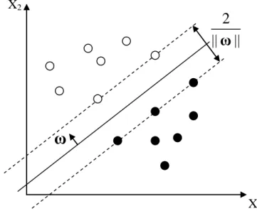
The Support Vector Machine (SVM) is a successfully parametric method, which has been widely used to get accurate results in many multiple-class pattern recognition applications. As introduced in [87-88], SVM, which fits to classify data of high dimensions and from multiple sources particularly, extends the use of kernels which are crucial to incorporate priori knowledge into practical applications.
A simplification is one-class SVM, which is derived from two-class situation SVM; in one-class SVM the training points just involve the class to be separated from others [89]. Other recent developments have shown the benefits of multi-kernel SVM [90-91]. Multi-kernel SVM has more potential for fusion of the data from heterogeneous sources at the expense of computation complexity. It has been proven in [92] that, when the kernel function can be decomposed into a large sum of individual and basic kernels which can be embedded in a directed acyclic graph, the penalty functions can be explored by sparsity-inducing norms such as the l1-norm.
1.4 Work of This Paper
Currently, there are still many outstanding issues in the medical images-based, particularly MRI images-based brain tumor detection, such as the huge amount of data in MRI examination, heavy burden of the computation, data of high dimensionality, complex characteristics of tissues, the difficulty in classifier design, large differences among individual patients, the infeasibility of establishing a fully automated system, no prior knowledge of the patient’s condition to use, a variety of tissues in the tumor region, the overlapping of the boundaries between normal tissues and abnormal tissues which is difficult to be distinguished and so on.
As to these problems and some limitations of existing methods, this paper proposes a semi-automatic SVM-based system to achieve the detection and track of the brain tumors, which can classifies the tumors and abnormal tissues gradually. The system consists of three subsystems, including three main abilities of classification, contour refinement and tracking. The input data of the system are the fusion of T2-weighted images, PD-weighted images and FLAIR-weighted images. The feature vectors are extracted using the characteristics of the weighted sequence of their own and that of correlation between several sequences. Feature selection can fuse and reduce the data effectively and multi-kernel SVM is applied for a variety of data input to improve the accuracy of tumor detection. At the same time the system can effectively track the condition of patients after the first detection of tumors and give reasonable diagnosis conclusion as a reference.
This paper contains five sections, which is organized as follows: Chapter 1 is the introduction, which introduces the background and significance of the subject, the principle and theory of magnetic resonance imaging, and the summary of existing tumor detection algorithms. Chapter 2 proposes a method to integrate the feature selection and classifier’s design, and describes in detail all the feature selection methods used in the
experiments of this paper. Chapter 3 describes the proposed tumor detection system and the three subsystems of classification, contour refinement and trackingare also described in detail. Chapter 4 lists the results of this paper and discusses a variety of situations, including the validity of features, the selection of key parameters, the comparison among methods, and the evaluation of the system’s performance. Chapter 5 concludes the full text, proposes the improvement goals of the system and finally states the future development of this subject.
CHAPTER 2 FEATURE SELECTION
2.1 Feature Selection Theory
Feature selection is an important data processing step in pattern recognition and classification problems, and it has been successfully applied to many fields [93-97]. The procedure of feature selection is as follows: in accordance with pre-designed selection criteria, the most important features of the given input data are selected by the optimal operations under the prefixed criterion and the remaining features are removed from the input to reduce the data amount.
Although the applied classification fields are different, the ultimately obtained signal is overlapped with a lot of interference and noise in the specific pattern recognition and classification problems, due to the inevitable signal loss and introduced interference in the process of equipment’s acquisition, imaging environment, data transmission and conversion. In addition to the traditional denoising algorithms, feature selection, as an important pre-processing operation, plays an important role in the data pre-processing:
1. Feature selection can eliminate the redundancy, interference, noise and less important data in input. According to the definition of feature selection, this process can choose the data based on some certain criteria to eliminate all the factors which are not relative to the classification problems, and to effectively fuse the important data and therefore greatly reduce the data amount.
2. Feature selection can improve the accuracy of the classifier. After the feature selection operation, a large number of non-relevant data which contain many interferential components are removed. Only the most important features are remained for training, which makes the obtained classification model much better to improve the applicability of the model and its ability for solving the problem, and finally to achieve higher classification accuracy.
3. Feature selection can improve the operational efficiency. After the feature selection, the training sample data greatly decrease and the computational complexity is reduced in a relatively lower degree (mainly determined by the algorithm, thus changes on the computational complexity by reducing the amount of data is just in a relative sense) to reduce the computation time.
Because of the importance of feature selection in the pattern classification problems feature selection has been a hot point and difficult issues in this research area. How to determine an effective feature selection criterion, to extract the important features and to verify the validity, reliability, applicability, robustness and computational
efficiency of the criterion by experiments are the key problems to be solved [98-103]. Commonly used feature selection framework are shown in Figure 2.1 [95].
Figure 2.1 A typical framework of feature selection.
A typical feature selection process is divided into 3 steps [95]:
1. Subset Generation: this is the process to conditionally extract the feature subset from the training feature vector matrix prepared for being analyzed by the classifier or a single vector according to some certain criteria. The feature subset will be considered as the result of one step of the feature selection operation to evaluate its performance of feature selection.
2. Subset Evaluation: feature selection can be fulfilled in two directions: one is to begin with a feature subset which contains just one element and to increase the capacity of the subset element by element; the other is to begin with a universal set which contains all the elements of the feature subset and to decrease the capacity of the subset element by element. No matter what kind of direction is used for the feature selection, the effectiveness of the current subset is needed to evaluate once the feature subset changes in a time. The evaluation process of feature selection is to be completed by the pre-set criterion.
3. The determination of the stop criterion: each feature subset after assessing is needed to be compared with the stopping criterion to verify if the characteristics of the current subset have attained a pre-set standard. If so, feature selection will stop automatically and the current subset will be considered as the final output; otherwise this process will continue to repeat again and again until a feature subset which meets the stopping criterion appears. This is an optimization process, and the algorithm sometimes does not automatically converge due to the restrictions of the feature selection criteria and the stopping criteria. Therefore, the stopping criteria maybe need to be set manually (such as setting a limited number of iteration steps). This also indicates that the feature selection criteria and the stopping criteria
Input Set
Subset Generation Subset Subset Evaluation Criterion Comparison
Stop Criterion? No
Yes Result Output
will significantly affect and restrict the efficiency, performance and accuracy of the feature selection operations.
As a number of MRI sequences present a three-dimensional structure and each MRI sequence also contains multiple images, which leads to a large amount of data, dimensionality reduction of data by feature selection is particularly necessary. In this paper, a SVM-based tumor detection framework is designed to analysis and deal with the MRI sequences. The difficulties lie in the design of the SVM classifier, the selection of the kernel function and its parameters. Therefore, the algorithm to integrate the feature selection and classifier design is proposed in this paper as a pre-processing step, the key of which is trying to improve the accuracy and efficiency of the system while reducing the dependence of SVM to the kernel function parameter, the difficulty of classifier design and the influence of parameters on the classifier design by the feature selection process.
For these purposes of the effective fusion of data and the verification of the proposed algorithm to reduce the difficulties of parameter selection in classifier design by the feature selection process, we selected 6 novel feature selection methods in the experimentations of tumor detection. The performances and effectivenessof the feature selection methods above is evaluated and compared by visual results and quantitative analysis.
The feature selection methods will be introduces in detail in the next section.
2.2 Feature Selection Algorithms
2.2.1 Principal Component Analysis
Principal Component Analysis ( PCA) is a classic feature selection method [104], which uses the projection transformation to project the input data from the original space into the new space. The axises in the new space correspond to the projection direction and all the axes maintain the orthogonal relationship. Projection direction can be obtained from the diagonalization transformation of the raw data, therefore the projectieddata will be all located in the axis in the new space.
The value of each new axis can be considered as the energy of the data, then the sum of all the coordinates is all the included energy of the original input data. Align the coordinate values in a descending order to choose the first n values, the sum of which reaches 95% of the total energy and discard the remaining coordinates, therefore, the axes the remained coordinates correspond to are the principal directions in the new space after the projection.
The ratio of the energy can be manually set, which always changes in a range from 85% to 99%. Reflected in the projected data, the larger eigenvalues are retained in the transformed diagonal matrix, the small ones are removed, and the sum of the retained eigenvalues reaches the proportion of the total values. Although the vast majority of
energy reserves, the new space just contains only a very few of axes, which are the corresponding principal components. PCA is significantly based on the principle of energy concentration to achieve the purpose of data reduction through the projection transformation.
The implementation of PCA is often based on the SVD decomposition, the key of which is to obtain the spatial projection transformation matrix. Each row of the matrix above corresponds to the eigenvectors of the matrix after the projection. Set xi as the
input sample vector, μ as the mean vector for all the input sample vectors, which is composed of the mean values of all the various components arranged in the order in accordance with the corresponding vector, see equation (2-1).
1 1 M j ij i x M
(2-1)Where j and x are the j -th element of ij x and i μ respectively and M is
total number of training samples. Define:
1 2
[ ; ; ; M ]
X x μ x μ x μ (2-2)
The semicolon indicates the separation between the row vectors, which is the row vectorxiμ of the matrix X, respectively.
The covariance matrix Σ of X is:
T T 1 1 1 ( )( ) M M M i i i M M
Σ x μ x μ XX (2-3)Let the eigenvalues of Σ be i , then the row vector of the projection transformation matrix is the eigenvector u of i Σ, which is orthonormalized and corresponds to i. u can be solved through matrix R and its eigenvector i v . i
Define R as: T 1 M M M R X X (2-4)
R and Σ contain the same eigenvalues of i, and there is a mathematical relationship between u and i v : i
/
i i i
u Xv (2-5)
Therefore, the projection transformation matrix is:
1 2
[ ; ; ; i; ; n]
T u u u u (2-6)
In PCA-based data classification, the first step is to calculate the projection transformation matrix to project the original input data to the new space, and then to
train the classifier model by using the data after dimensionality reduction. Test data must be dealt with by the same dimension reduction transformation to obtain the same data format as the training samples and the classification model can be finally applied.
PCA algorithm is quick, easy and simple (without high complexity). After the dimension reduction of PCA algorithm, only a very small part of the original input data is preserved, which correspond to a finite number of the largest eigenvalues of the matrix R in the equation (2-4). Projection transformation just changes the form of data, but not the energy of data. Therefore, the eigenvalues after transformation contain most of the energy in the original image, that is to say, there is no energic loss of information in the original image, which will not influence the classification to a great degree.
The disadvantage of PCA algorithm is its low accuracy. As the complexity of data increases, its accuracy can not be surely guaranteed.
2.2.2 Kernel PCA
Kernel Principal Component Analysis (Kernel PCA, or KPCA) is an effective extention of PCA algorithm [105], which is also widely used in various fields of pattern recognition and classification [106-108]. The main idea of Kernel PCA is to apply PCA directly to the kernel space or feature space. First define the kernel function as:
( , )i j ( ), ( )i j ( ( ) ( ))i j
k x x =< Φ x Φ x >= Φ x ⋅Φ x (2-7) Φ is to map transformation from the original input data to a higher-dimensional space (ie the kernel space or feature space), xi and xj are the original input data,
< ⋅ > denotes the inner product of two vectors. From Equation (2-7), the result of kernel
function is a scalar value, which can be measured as the distance between two vectors to some extent. The closer the distance is, the higher the similarity between vectors is. The basic definition of the kernel function can be applied to all kernel function-based methods in the next sections of this paper.
Refered to the SVD method on the implementation of PCA, the input vector becomes to Φ( )xi in high dimensional feature space, and the corresponding covariance
matrix is: T 1 1 M ( )[ ( )] i i i M = =
∑
Φ Φ C x x (2-8)The projection transformation matrix of PCA in the feature space is composed of normalized eigenvectors of the matrix C. To solve the eigenvalues and eigenvectors,
the equation as follows is needed to be solved:
λu Cu= (2-9)
λ and u are the eigenvalues and eigenvectors of the matrix C respectively. It
Since any vector in the linear space can be expressed as a linear combination of other vectors, the eigenvectors u can be expressed by a linear combination of each
( )i
Φ x . Suppose αi is the coefficients of the linear combination, then:
1 ( ) M i i i α = =
∑
Φ u x (2-10)Pre-multiply Φ( )xk at the both ends of the Equation (2-9), and substitute
Equations (2-7), (2-8) and (2-10) into (2-9), then we can get: 1 1 1 1 ( , ) ( , ) ( , ) M M M i k i i k i i j i i j M k k k M λ α α = = = ⋅ = ⋅ ⋅
∑
x x∑∑
x x x x (2-11)Construct the inner product matrix K and the coefficient vector α . Each element
of K is an inner product of two input vectors, ie,Kij =k( , )x xi j =< Φ( ), ( )xi Φ xj > and
1 2
( , , ,α α αM) =
α , then Equation (2-11) can be rewritten as:
2
M λKα K α= (2-12) Pre-multiply K at the both ends of Equation (2-12): −1
Mλα Kα= (2-13)
From (2-13), this equation is equal to solve the eigenvalues M λ of the matrix K
which corresponds to the eigenvectors α . All the eigenvectors corresponding to the non-zero eigenvalues can form the projection transformation matrix after normalization.
In the realization of Kernel PCA algorithm, first calculate the inner product of the various samples according to the given input samples to construct the inner product matrix K; and then calculate its eigenvalues and eigenvectors to obtain the projection transformation matrix; finally, obtain the principal component projection in the feature space for any input test sample. The whole procedure is very similar to PCA.
Kernel PCA algorithm tries to solve the complex classification problem by mapping from the low-dimensional space into high-dimensional feature space. In general, the difficulty of classification will greatly decrease, and data which can not be separated in low-dimensional space can be linearly separable in high-dimensional space. Algorithm introduces an inner product function, which ensure the feature space must be a Hilbert space and the operations in this space can be completely achieved through the inner product instead of calculation and solution of the unknown mapping. The restriction of the algorithm is its need to pre-selected the kernel function and its corresponding parameters. The selection process will also greatly affect the effectiveness of the algorithm.
2.2.3 Kernel Class Separability
Kernel Class Separability (KCS) is the extention of commonly used traditional class separability in pattern recognition and classification into a kernel space or feature