Vision-Aided Inertial Navigation : low computational complexity algorithms with applications to Micro Aerial Vehicles

HAL Id: tel-01548441

https://tel.archives-ouvertes.fr/tel-01548441

HAL is a multi-disciplinary open access

archive for the deposit and dissemination of sci-entific research documents, whether they are pub-lished or not. The documents may come from teaching and research institutions in France or

L’archive ouverte pluridisciplinaire HAL, est destinée au dépôt et à la diffusion de documents scientifiques de niveau recherche, publiés ou non, émanant des établissements d’enseignement et de recherche français ou étrangers, des laboratoires

Vehicles

Chiara Troiani

To cite this version:

Chiara Troiani. Vision-Aided Inertial Navigation : low computational complexity algorithms with applications to Micro Aerial Vehicles. Robotics [cs.RO]. Université de Grenoble, 2014. English. �NNT : 2014GRENM021�. �tel-01548441�

THÈSE

Pour obtenir le grade de

DOCTEUR DE L’UNIVERSITÉ DE GRENOBLE

Spécialité : Mathématiques-informatique Arrêté ministériel : 7 août 2006

Présentée par

Chiara TROIANI

Thèse dirigée par Christian Laugier codirigée par Agostino Martinelli

préparée au sein du centre de recherche INRIA Rhône-Alpes, du Laboratoire d’Informatique de Grenoble

dans l'École Doctorale Mathématiques, Sciences et

Technologies de l’Information, Informatique

Vision-Aided Inertial

Navigation : low computational

complexity algorithms with

applications to Micro Aerial

Vehicles

Thèse soutenue publiquement le 17 Mars 2014, devant le jury composé de :

Simon LACROIX

Directeur de Recherche LAAS/CNRS, Toulouse, France, Rapporteur

Gianluca ANTONELLI

Professeur Universitá degli Studi di Cassino, Italie, Rapporteur

Christian LAUGIER

Directeur de Recherche INRIA Rhône-Alpes, Grenoble, France, Directeur de thèse

Agostino MARTINELLI

Chargé de Recherche INRIA Rhône-Alpes, Grenoble, France, Co-Directeur de thèse

Davide SCARAMUZZA

Professeur University of Zurich, Suisse, Examinateur (et Co-Encadrant)

Fabien BLANC-PAQUES

To my Mum and Dad, because without their love and support nothing would have been possible.

Matt Might, a Professor of Computer Science at University of Utah, described what a doctorate is in the following way:

1. Imagine a circle that contains all of human knowledge;

2. By the time you finish elementary school, you know a little;

3. By the time you finish high school, you know a bit more;

4. With a bachelor’s degree, you gain a specialty;

5. A master’s degree deepens that specialty;

6. Reading research papers takes you to the edge of human knowledge;

7. Once you’re at the boundary, you focus;

8. You push at the boundary for a few years;

9. Until one day, the boundary gives way;

10. And, that dent you’ve made is called a PhD;

11. Of course, the world looks different to you now;

12. So, don’t forget the bigger picture:

13. Keep pushing.

Going through a PhD is a long travel which passes over all those steps, each transition was an important moment, and in each of those moments I had the inestimable chance to be surrounded by people

who supported me, who coached me, who trusted me, who helped me. Now, sorry if those couple of pages will not have a “formal shape”, but this is for me the best moment of my three years of PhD: the moment in which I can finally thank all the people who made this possible.

I would like to start thanking my supervisor, Agostino Martinelli, for the support, the patience, the advices, the interesting discussions, his epic stories and for allowing me to defend my thesis even if I didn’t go yet on the top of the “Mont Blanc”. Thanks to my co-supervisor Davide Scaramuzza for hosting me 8 months in his lab in Zurich, for all the discussions and the feedbacks and thanks because the 8 months spent at the AI Lab gave me also the big gift of a dear friend. Thanks to my thesis director Christian Laugier, for his guidance and for being an example of leader to follow under not only a working but also a human point of view. Thanks to Simon Lacroix and Gianluca Antonelli who accepted to review my thesis and to Fabien Blanc-Paques who allowed me to collaborate with his company and accepted to be member of my commitee.

Thanks to e-motion, because e-motion is not only an Inria’s team, it is my Team, it is family, friends, work and amusement. Thanks to Myr-iam, because without Myriam there would not exist any e-motion, because each team needs its Myriam, but everybody who leaves e-motion realizes that there exist only one Myriam: ours! Thanks to SG (or “services g´en´ereux”, as I have always called them, Ger-ard, Alain, Ben), because they are simply extraordinary. Thanks to Stephanie for... well, there would be too much to write, let’s simply say: thanks for being always present even miles far away. Thanks to Alex and Matina for all the moments we spent together, the cooking, the hikings, the movies. Thanks to Jorge, because he survived “dans le bureau des filles” without going crazy and because now that this office became again “le bureau des filles”, we really feel that there is someone missing. To Karla for all the times she knocked at my door with her delicious Mexican dishes, to Lota: my favourite helicopter pilot, to Dizan, Barbara, Manu, Amaury, Stephanie, Alessandro, Ar-turo, Procopio, Mike, Anne, Lukas, Juan, Juan David and more gen-erally to all the e-motion team for all the moments shared, for all the coffee-breaks and especially for the support all of you gave me from the beginning until the end of this experience!

Thanks to the sFly team: I learned a lot from all of you! Thanks to my officemates in Zurich, Flavio, Mathias, Elias, Matia and Christian

and to the people of “anche a Zurigo un angolo di cielo pu´o essere rotondo” (Spalla, Bocci, Pippo, Prest, Spampi, Ale).

Thanks to my Professor, Costanzo Manes, for transmitting me his passion for robotics, for encouraging me to apply for a PhD and for recommending me to come here. Thanks to Paolo, for the constant on-line support and for the “insults” when I brake the batteries of my helicopter.

Thanks to my Family who gave me the stability and calm necessary to grew up and became what I am today. To my Dad, “sperando che un giorno riuscir´o ad assomigliargli almeno un po’ ”, and to my Mum, because “le somiglio gi´a tantissimo e ne sono fiera!”. To my sister because even if she will always be “la mia piccolina”, I had and I will always have a lot to learn from her. Thanks to Matteo, because he has always been and I know he will always be present. Thanks to Andrea for his “sixth sense” about knowing whenever I may need something and because “se c’´e un fiocco ´e grazie a lui!”. Thanks to Nicole and Claude, because all the latest news I got about drones were coming from them and because “c’est beau de pouvoir se sentir en famille mˆeme `a mille kilometres de chez moi”.

And last but absolutely not least: thanks to Mathias for being at my side from the beginning to the end of this experience acquiring a constantly growing role, for all his precious advices and his patience but especially for giving to this thesis a special additional significance.

Abstract

Accurate egomotion estimation is of utmost importance for any navigation sys-tem. Nowadays different sensors are adopted to localize and navigate in unknown environments such as GPS, range sensors, cameras, magnetic field sensors, inertial sensors (IMU). In order to have a robust egomotion estimation, the information of multiple sensors is fused. Although the improvements of technology in provid-ing more accurate sensors, and the efforts of the mobile robotics community in the development of more performant navigation algorithms, there are still open challenges. Furthermore, the growing interest of the robotics community in mi-cro robots and swarm of robots pushes towards the employment of low weight, low cost sensors and low computational complexity algorithms. In this context inertial sensors and monocular cameras, thanks to their complementary charac-teristics, low weight, low cost and widespread use, represent an interesting sensor suite.

This dissertation represents a contribution in the framework of vision-aided inertial navigation and tackles the problems of data association and pose estima-tion aiming for low computaestima-tional complexity algorithms applied to MAVs.

For what concerns the data association, a novel method to estimate the rela-tive motion between two consecurela-tive camera views is proposed. It only requires the observation of a single feature in the scene and the knowledge of the angu-lar rates from an IMU, under the assumption that the local camera motion lies in a plane perpendicular to the gravity vector. Two very efficient algorithms to remove the outliers of the feature-matching process are provided under the above-mentioned motion assumption. In order to generalize the approach to a 6DoF motion, two feature correspondences and gyroscopic data from IMU measure-ments are necessary. In this case, two algorithms are provided to remove wrong data associations in the feature-matching process. In the case of a monocular camera mounted on a quadrotor vehicle, motion priors from IMU are used to discard wrong estimations.

For what concerns the pose estimation problem, this thesis provides a closed form solution which gives the system pose from three natural features observed in a single camera image, once the roll and the pitch angles are obtained by

pattern formed by the three features.

In order to tackle the pose estimation problem in dark or featureless environ-ments, a system equipped with a monocular camera, inertial sensors and a laser pointer is considered. The system moves in the surrounding of a planar surface and the laser pointer produces a laser spot on the abovementioned surface. The laser spot is observed by the monocular camera and represents the only point feature considered. Through an observability analysis it is demonstrated that the physical quantities which can be determined by exploiting the measurements provided by the aforementioned sensor suite during a short time interval are: the distance of the system from the planar surface; the component of the system speed that is orthogonal to the planar surface; the relative orientation of the sys-tem with respect to the planar surface; the orientation of the planar surface with respect to the gravity. A simple recursive method to perform the estimation of all the aforementioned observable quantities is provided. This method is based on a local decomposition of the original system, which separates the observable modes from the rest of the system.

All the contributions of this thesis are validated through experimental results using both simulated and real data. Thanks to their low computational com-plexity, the proposed algorithms are very suitable for real time implementation on systems with limited on-board computation resources. The considered sensor suite is mounted on a quadrotor vehicle but the contributions of this dissertations can be applied to any mobile device.

R´

esum´

e

L’estimation pr´ecise du mouvement 3D d’une cam´era relativement `a une sc`ene rigide est essentielle pour tous les syst`emes de navigation visuels. Aujourd’hui diff´erents types de capteurs sont adopt´es pour se localiser et naviguer dans des en-vironnements inconnus : GPS, capteurs de distance, cam´eras, capteurs magn´etiques, centrales inertielles (IMU, Inertial Measurement Unit). Afin d’avoir une estima-tion robuste, les mesures de plusieurs capteurs sont fusionn´ees. Mˆeme si le progr`es technologique permet d’avoir des capteurs de plus en plus pr´ecis, et si la com-munaut´e de robotique mobile d´eveloppe algorithmes de navigation de plus en plus performantes, il y a encore des d´efis ouverts. De plus, l’int´erˆet croissant des la communaut´e de robotique pour les micro robots et essaim de robots pousse vers l’emploi de capteurs `a bas poids, bas coˆut et vers l’´etude d’algorithmes `a faible complexit´e. Dans ce contexte, capteurs inertiels et cam´eras monoculaires, grˆace `a leurs caract´eristiques compl´ementaires, faible poids, bas coˆut et utilisation g´en´eralis´ee, repr´esentent une combinaison de capteur int´eressante.

Cette th`ese pr´esente une contribution dans le cadre de la navigation inertielle assist´ee par vision et aborde les probl`emes de fusion de donn´ees et estimation de la pose, en visant des algorithmes `a faible complexit´e appliqu´es `a des micro-v´ehicules a´eriens.

Pour ce qui concerne l’association de donn´ees, une nouvelle m´ethode pour estimer le mouvement relatif entre deux vues de cam´era cons´ecutifs est propos´ee. Celle-ci ne n´ecessite l’observation que d’un seul point caract´eristique de la sc`ene et la connaissance des vitesses angulaires fournies par la centrale inertielle, sous l’hypoth`ese que le mouvement de la cam´era appartient localement `a un plan per-pendiculaire `a la direction de la gravit´e. Deux algorithmes tr`es efficaces pour ´

eliminer les fausses associations de donn´ees (outliers) sont propos´es sur la base de cette hypoth`ese de mouvement. Afin de g´en´eraliser l’approche pour des mou-vements `a six degr´es de libert´e, deux points caracteristiques et les donn´ees gyro-scopiques correspondantes sont n´ecessaires. Dans ce cas, deux algorithmes sont propos´es pour ´eliminer les outliers. Nous montrons que dans le cas d’une cam´era monoculaire mont´ee sur un quadrotor, les informations de mouvement fournies par l’IMU peuvent ˆetre utilis´ees pour ´eliminer de mauvaises estimations.

et le tangage sont obtenus par les donn´ees inertielles sous l’hypoth`ese de ter-rain plan. Plus sp´ecifiquement, la position et l’attitude du syst`eme peuvent ˆetre uniquement d´etermin´ees `a partir de l’observation de deux points caract´eristiques, mais am´elior´ees en exploitant les contraintes g´eom´etriques inh´erentes `a un pattern virtuel form´e par les trois points caract´eristiques.

Afin d’aborder le probl`eme d’estimation de la pose dans des environnements sombres ou manquant de points caract´eristiques, un syst`eme ´equip´e d’une cam´era monoculaire, d’une centrale inertielle et d’un pointeur laser est consid´er´e. Le syst`eme se d´eplace dans l’entourant d’une surface plane et le pointeur laser pro-duit un petit point sur la surface. Le point laser est observ´e par la cam´era monoculaire et repr´esente le seul point caract´eristique consid´er´e. Grˆace `a une analyse d’observabilit´e il est d´emontr´e que les grandeurs physiques qui peuvent ˆ

etre d´etermin´ees par l’exploitation des mesures fourni par ce systeme de capteurs pendant un court intervalle de temps sont : la distance entre le syst`eme et la surface plane ; la composante de la vitesse du systme qui est orthogonale `a la surface ; l’orientation relative du syst`eme par rapport `a la surface et l’orientation de la surface par rapport `a la gravit´e. Une m´ethode r´ecursive simple a ´et´e pro-pos´ee pour l’estimation de toutes ces quantit´es observables. Cette m´ethode est bas´ee sur une d´ecomposition locale du syst`eme d’origine, qui s´epare les modes observables du reste du syst`eme.

Toutes les contributions de cette th`ese sont valid´ees par des exp´erimentations `

a l’aide des donn´ees r´eelles et simul´ees. Grace `a leur faible complexit´e de calcul, les algorithmes propos´es sont tr`es appropri´es pour la mise en oeuvre en temps r´eel sur des syst`emes ayant des ressources de calcul limit´ees. La suite de capteur consid´er´ee est mont´e sur un quadrotor, mais les contributions de cette th`ese peuvent ˆetre appliqu´ees `a n’importe quel appareil mobile.

Contents

Contents ix

List of Figures xii

1 Introduction 1

1.1 Context . . . 1

1.1.1 Why quadrotors? . . . 2

1.1.2 Brief quadrotor’s history . . . 3

1.1.3 Applications . . . 4

1.1.4 The quadrotor concept . . . 4

1.2 Motivation and objectives . . . 6

1.2.1 Minimalist perception . . . 9

1.3 Contributions . . . 10

1.4 Thesis outline . . . 12

2 Visual and Inertial sensors 13 2.1 A biological overview . . . 14

2.1.1 The sense of sight . . . 14

2.1.2 The perception of gravity . . . 15

2.2 Inertial Measurement Unit . . . 17

2.2.1 Accelerometers . . . 18

2.2.2 Gyroscopes . . . 19

2.3 Camera . . . 20

2.3.1 Pinhole Camera Model . . . 21

2.4 Camera Calibration . . . 23

2.5 Camera-IMU Calibration . . . 24

3 Data association 27 3.1 Feature extraction and matching . . . 28

3.1.1 Feature Detection . . . 28

3.1.3 Feature Matching . . . 30

3.2 Outlier detection . . . 31

3.2.1 Related works . . . 32

3.2.2 Epipolar Geometry . . . 33

3.2.3 1-point algorithm . . . 34

3.2.3.1 Parametrization of the camera motion . . . 34

3.2.3.2 1-point Ransac . . . 37

3.2.3.3 Me-RE (Median + Reprojection Error) . . . 37

3.2.3.4 Performance evaluation . . . 37

3.2.3.5 Conclusions . . . 42

3.2.4 2-point algorithm . . . 45

3.2.4.1 Parametrization of the camera motion . . . 45

3.2.4.2 Hough . . . 47

3.2.4.3 2-point Ransac . . . 48

3.2.4.4 Quadrotor motion model . . . 49

3.2.4.5 Performance evaluation . . . 51

3.2.4.6 Conclusions . . . 55

4 Pose estimation 59 4.1 Filtering approaches and closed form solutions . . . 60

4.2 Virtual patterns . . . 61

4.2.1 The System . . . 62

4.2.2 The method . . . 63

4.2.2.1 2p-Algorithm . . . 63

4.2.2.2 3p-Algorithm . . . 66

4.2.2.3 Scale factor initialization . . . 67

4.2.2.4 Estimation of γ1 and γ2 . . . 71 4.2.3 Performance Evaluation . . . 71 4.2.3.1 Simulations . . . 71 4.2.3.2 Experimental Results . . . 72 4.2.4 Conclusion . . . 75 4.3 Virtual features . . . 77 4.3.1 The System . . . 78

4.3.2 Camera-laser module calibration . . . 81

4.3.3 Observability Properties . . . 82

4.3.4 Local Decomposition and Recursive Estimation . . . 86

4.3.5 Performance Evaluation . . . 88

4.3.5.1 Simulations . . . 89

4.3.5.2 Preliminary experiments . . . 91

4.3.5.3 Camera-laser module calibration . . . 95

CONTENTS

5 Conclusions 97

5.1 Research Outlook . . . 99

Bibliography 100

1.1 MAVs classification. The vehicles in the pictures are: Perching Glider, MIT (a); Festo’s Smartbird (b); AeroVironments Nano Hummingbird (c); Skybotix’s CoaX (d); Parrot’s AR.Drone (e). . 2

1.2 History of quadrotors with respect to their application fields. 1907: Paul Corny machine (both from 1907), Br´eguet Giant Gyroplane. 1924: Ohemichen’s quadrotor; 2000: ETH Zurich’s OS4 [16], [15], the CEA’s X4-flyer [37] and the ANU’s X-4 Flyer [79]; Nowadays there exists a lot of quadrotors. We list here few exemplars: AscTec Pelican [1], KMelRobotics’ NanoQuad [3], Mikrokopter’s quadro-tor [4], Flyduino, Arducopter, Parrot AR.Drone, DeltaDrone quadro-tor [2]. . . 3

1.3 Quadrotors in research projects and in companies. . . 5

1.4 Quadrotor notation. The four rotors are depicted in blue. wi is the angular velocity of the i-th rotor, Fi and Mi are the vertical force and the moment respectively produced by the i-th rotor. The body-vehicle’s frame B is shown in black, it is attached to the vehicle, and its origin is coincident with the vehicle’s center of mass. In gray it is depicted the world reference frame W. . . 6

1.5 The quadrotor concept. The width of the arrows is proportional to the angular speed of the propellers. . . 7

1.6 Properties of some sensors commonly on-board a MAV. . . 8

1.7 Flight Assembled Architecture (a) at FRAC Centre in Orlans, France [25]. Robot Quadrotors Perform James Bond Theme (b) [53]. Figure (c) represents a motion capture system room. Figures (a),(c) courtesy of http://www.flyingmachinearena.org. . . 9

1.8 This table summarises the objective of this dissertations in terms of minimalist perception. . . 10

2.1 Complementary properties of cameras and IMU sensors. . . 14

2.2 Human eye. Image courtesy of http://www.biographixmedia.com. 15

LIST OF FIGURES

2.4 Vestibular system. Image (a) courtesy ofhttp://www.chrcentre.

com.au, image (b) courtesy of http://biology.nicerweb.com. . 17

2.5 Halteres: small knobbed structures in some two-winged insects. They are flapped rapidly and function as gyroscopes, providing informations to the insect about his body rotation during flights. . 17

2.6 IMU applications Image courtesy ofhttp://www.unmannedsystemstechnology. com. . . 18

2.7 Physical principle of a single-axis accelerometer. . . 19

2.8 Scheme of a 3D mechanical Gyroscope. Image courtesy of http: //www.wikipedia.org. . . 20

2.9 Diagram of a CCD (a) and CMOS (b) sensor. . . 21

2.10 Matrix Vision mvBlueFOX-MLC usb camera. . . 22

2.11 Pinhole camera model for standard perspective cameras. . . 22

2.12 Chessboard images used for calibration. . . 24

2.13 Extracted corners on a chessboard. . . 25

2.14 Camera and IMU observing the vertical direction. Redrawn from [57]. . . 25

2.15 Camera poses relative to the calibration chessboard (a). Results of rotation estimation (b). . . 26

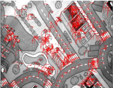
3.1 Comparison of feature detectors: properties and performances [88]. 30 3.2 Surf features matched across multiple frames overlaid on the first image. . . 31

3.3 Number of RANSAC iterations. . . 32

3.4 Epipolar constraint. p1, p2, T and P lie on the same plane (the epipolar plane). . . 33

3.5 Notation. . . 35

3.6 Cp1and Cp2are the reference frames attached to the vehicle’s body frame but which z-axis is parallel to the gravity vector. They correspond to two consecutive camera views. Cp0 corresponds to the reference frame Cp1 rotated according to dY aw. . . 36

3.7 Synthetic scenario. The green line represents the trajectory and the red dots represent the simulated features. . . 39

3.8 Number of found inliers by Me-RE (red), 1-point RANSAC (cyan), 5-point RANSAC (black), true number of inliers(blue) for a perfect planar motion. . . 39

3.9 Number of found inliers by Me-RE (red), 1-point RANSAC (cyan), 5-point RANSAC (black), true number of inliers(blue) in presence of perturbations on the Roll and P itch angles. . . 40

3.10 Number of found inliers by Me-RE (red), 1-point RANSAC (cyan), 5-point RANSAC (black), true number of inliers(blue) in presence of perturbations on the dY aw angle. . . 40

3.11 Number of found inliers by Me-RE (red), 1-point RANSAC (cyan), 5-point RANSAC (black), true number of inliers(blue) for a non-perfect planar motion (s1 = 0.02 ∗ sin(8 ∗ wc· t)). . . 41 3.12 Nano quadrotor from KMelRobotics: a 150g and 18cm sized

plat-form equipped with an integrated Gumstix Overo board and Ma-trixVision VGA camera. . . 41

3.13 Plot of the real trajectory. The vehicle’s body frame is depicted in black and the green line is the trajectory followed. . . 43

3.14 Number of found inliers by Me-RE (red), 1-point RANSAC (green), 5-point RANSAC (black), 8-point RANSAC (blue) along the tra-jectory depicted in Figure 3.13. . . 43

3.15 From the top to the bottom: Roll, P itch and dY aw angles [deg] estimated with the IMU (red) versus Roll, P itch and dY aw an-gles [deg] estimated with the Optitrack system (blue). The last plot shows the height of the vehicle above the ground (non perfect planarity of motion). . . 44

3.16 Computation time. . . 45

3.17 The reference frame C0 and C2 differ only for the translation vector T . ρ = |T | and the angles α and β allow us to express the origin of the reference frame C2 in the reference frame C0. . . 46 3.18 Hough Space in α and β computed with real data. . . 48

3.19 Notation. . . 49

3.20 Motion constraints on a quadrotor relative to its orientation. ∆φ > 0 implies a movement along YB0 positive direction, ∆θ < 0 implies

a movement along YB0 positive direction. . . 50

3.21 Synthetic scenario. The red line represents the trajectory and the blue dots represent the simulated features. The green dots are the features in the current camera view. . . 52

3.22 The IMU measurements are not affected by noise (ideal conditions). 53

3.23 The angles ∆φ, ∆θ and ∆ψ are affected by noise. . . 53

3.24 Only the angles ∆φ and ∆θ are affected by noise. . . 54

3.25 Only the angle ∆ψ is affected by noise. . . 54

3.26 Real scenario. The vehicle body frame is represented in blue, while the red line represents the followed trajectory. . . 56

3.27 Number of inliers detected with the Hough approach (red), the 2-point RANSAC (cyan), the 5-point RANSAC (black) and the 8-point RANSAC (blue) along the trajectory depicted in Figure

LIST OF FIGURES

3.28 Computation time. . . 57

3.29 Errors between the relative rotations ∆φ (errR), ∆θ (errP), ∆ψ (errY) estimated with the IMU and estimated with the Optitrack. 58 4.1 Global frame. Two is the minimum number of point features which

allows us to uniquely define a global reference frame. P1 is the origin, the xG-axis is parallel to the gravity and P2 defines the xG-axis . . . 63 4.2 The 2p-algorithm. . . 64

4.3 The three reference frames adopted in our derivation. . . 64

4.4 The yaw angle (−α) is the orientation of the XN-axis in the global frame. . . 65

4.5 The triangle made by the 3 point features. . . 66

4.6 Flow chart of the proposed pose estimator . . . 67

4.7 Estimated x, y, z (a), and Roll, P itch, Y aw (b). The blue line indicate the ground truth, the green one the estimation with the 2p-Algorithm and the red one the estimation with the 3p-Algorithm 73

4.8 Mean error on the estimated states in our simulations. For the position the error is given in %. . . 74

4.9 AscTec Pelican quadcopter [1] equipped with a monocular camera. 74

4.10 Our Pelican quadcopter: a system overview . . . 75

4.11 Scenario: The AR Marker and the 3 balls are used only with the aim to get a rough ground truth. The AR Marker provides the camera 6DOF pose in a global reference frame according to our conventions. . . 76

4.12 Estimated position (a), respectively x, y, z and estimated attitude (b), respectively Roll, P itch, Y aw. The red lines represent the estimated values with the 3p-Algorithm, the blue ones represent a rough ground truth (from ARToolkit Marker). . . 76

4.13 Quadrotor equipped with a monocular camera, IM U and a laser pointer. The laser spot is on a planar surface and its position in the camera frame is obtained by the camera up to a scale factor. . 79

4.14 The original camera frame XY Z, the chosen camera frame X0Y0Z0 and the laser module at the position [Lx, Ly, 0] and the direction (θ, φ) (in the original frame) and position [L, 0, 0] and the direc-tion (0, 0) (in the chosen camera frame). . . 80

4.15 Camera-Laser module calibration steps. Figure (a) is the camera image containing the laser spot projected onto a checkerboard. In green the reference frame attached to the checkerboard. Figure (b) represents three different camera positions used during the calibra-tion process, the green grid represents the checkerboard and the red lines represent the reference frame attached to the checkerboard. 82

4.16 The Pelican quadcopter equipped with a monocular camera and a laser module. . . 83

4.17 A typical vehicle trajectory in our simulations. . . 90

4.18 Estimated α in absence (a) and in presence of bias (b) on the inertial data. Blue dots indicate ground true values while red discs indicate the estimated values. . . 91

4.19 Estimated P in absence (a) and in presence of bias (b) on the inertial data. Blue dots indicate ground true values while red discs indicate the estimated values. . . 92

4.20 Estimated R in absence (a) and in presence of bias (b) on the inertial data. Blue dots indicate ground true values while red discs indicate the estimated values. . . 92

4.21 Estimated v0 in absence (a) and in presence of bias (b) on the inertial data. Blue dots indicate ground true values while red discs indicate the estimated values. . . 93

4.22 Estimated d in absence (a) and in presence of bias (b) on the inertial data. Blue dots indicate ground true values while red discs indicate the estimated values. . . 93

4.23 Estimated α in the experiment. Blue dots indicate ground true values while red discs indicate the estimated values. . . 94

4.24 Estimated P (a) and R (b) in the experiment. Blue dots indicate ground true values while red discs indicate the estimated values. . 94

4.25 Estimated vo (a) and d (b) in the experiment. Blue dots indicate ground true values while red discs indicate the estimated values. . 95

4.26 The Pelican quadcopter equipped with a monocular camera and a laser module and passive markers. . . 95

Chapter 1

Introduction

Contents

1.1 Context . . . 1

1.1.1 Why quadrotors? . . . 2

1.1.2 Brief quadrotor’s history . . . 3

1.1.3 Applications . . . 4

1.1.4 The quadrotor concept . . . 4

1.2 Motivation and objectives . . . 6

1.2.1 Minimalist perception . . . 9

1.3 Contributions . . . 10

1.4 Thesis outline . . . 12

1.1

Context

In recent years, flying robotics has received significant attention from the robotics community. The ability to fly allows easily avoiding obstacles and quickly having an excellent birds eye view. These navigation facilities make flying robots the ideal platform to solve many tasks like exploration, mapping, reconnaissance for search and rescue, environment monitoring, security surveillance, inspection etc. In the framework of flying robotics, micro aerial vehicles (MAV) have a further advantage. Due to the small size they can also be used in narrow out- and indoor environment and they represent only a limited risk for the environment and people living in it.

Fixed-­‐wing   Flapping-­‐_wing  

Avian-­‐style   Insect-­‐_style  

Rotor  cra:   Coaxial   Mul=-­‐_rotor  

(a)

(b) (c) (d) (e)

Figure 1.1: MAVs classification. The vehicles in the pictures are: Perching Glider, MIT (a); Festo’s Smartbird (b); AeroVironments Nano Hummingbird (c); Sky-botix’s CoaX (d); Parrot’s AR.Drone (e).

1.1.1

Why quadrotors?

Micro aerial vehicles can be classified into: Fixed-wing, Flapping-wing and rotor-crafts [52] (Figure1.1). Fixed-wing vehicles are not very agile in three-dimensional complex environment. Flapping-wing vehicles can be divided into avian-style and insect-style vehicles [61]. The development of the former is strongly limited by the lack of knowledge about fluid-structure coupling and aeroelasticity. Insect-style flapping wing MAVs and rotor-craft can perform stationary flight and forward flight, which represents a significant advantage in terms of maneuverability. Nev-ertheless, insect-style flapping wing vehicles present an increasing complexity and it has not yet been demonstrated whether they can be considered more convenient than rotor crafts. The most common rotor craft configurations for MAVs are the Coaxial rotorcraft and the Quadrotor aircraft. The former is well represented by the Skybotix Coax [5], a vehicle equipped with two co-axial, counter-rotating rotors and a stabilizer bar and the quadrotor vehicles. Quadrotors, thanks to their fast reaction to external disturbances, light weight and low crash impact, inherent safety, compactness, simple mechanical design, easier maneuverability and controllability and ability to carry small payloads, are nowadays the best option.

1907   1924   1956   Nowadays   2000   Nowadays   •  Military   •  Military   •  Military   •  Academic  research   •  Search  &  Rescue   •  Aerial  mapping   •  Cinematography   •  Security   •  Precision  Farming   •  Remote  sensing   •  InspecFon  …  

Figure 1.2: History of quadrotors with respect to their application fields. 1907: Paul Corny machine (both from 1907), Br´eguet Giant Gyroplane. 1924: Ohemichen’s quadrotor; 2000: ETH Zurich’s OS4 [16], [15], the CEA’s X4-flyer [37] and the ANU’s X-4 Flyer [79]; Nowadays there exists a lot of quadro-tors. We list here few exemplars: AscTec Pelican [1], KMelRobotics’ NanoQuad [3], Mikrokopter’s quadrotor [4], Flyduino, Arducopter, Parrot AR.Drone, DeltaDrone quadrotor [2].

1.1.2

Brief quadrotor’s history

At the beginning of the 20th century the French scientist and academician Charles Richet built a small, unmanned helicopter. Although the vehicle was not success-ful, it inspired two of his students, Louis and Jaques Br´eguet, which in 1907, under his supervision, built the first quad-rotor (Figure1.2) [55]. At the same time, the French engineer Paul Corny, designed an other quadrotor vehicle (Figure 1.2). Both the machines were reported to have carried a pilot off the ground but both of them lacked in stability and didn’t have a proper control architecture.

In 1920, ´Etienne Ohemichen, an employee of the French Peugeot car company, built a quadrotor machine, with eight additional rotors for control and propulsion.

vehicle was considered the earliest mention of a complete quadrotor hovering vehicle in history (Figure 1.2).

In 1956, Marc Adam Kaplan designed the most successful of the early designs of the rotor-craft (the Convertawings Model A quadrotor). With this machine Kaplan proved the quadrotor concept and realized the first four-rotor helicopter able to perform successful forward flight. This helicopter was intended to be the prototype for a line of much larger civil and military quadrotor helicopters, but due to a lack of orders for commercial or military versions, the project was terminated.

At the beginning of the third millennium, quadrotors drew the attention of academic researchers in order to address the problems faced by small-scale UAVs. The ETH Zurich’s OS4 [16], [15], the CEA’s X4-flyer [37] and the ANU’s X-4 Flyer [79] represents the first quadrotor research platforms.

1.1.3

Applications

Estimates from UAV Market Research (2011) reveals that the UAV market is estimated to exceed US$60 bilion in the next three years, and this forecast does not take into account for the thousands of MAVs already fielded.

As illustrated in Section1.1.2, the development of quadrotors has been boosted by the military (Figure 1.2). Nowadays, considering the high number and variety of research projects involving quadrotors and of companies already selling ready-to-flight products, their application field is widely extended (Figure1.3). Quadro-tor vehicles result suitable for search and rescue operations [69], [84], powerline inspection [39], [81], and building inspection, crop dusting, precision farming, re-mote sensing, security related tasks, aerial mapping, aerial photography, aerial delivery and cinematography tasks.

As stated by Vijay Kumar in [52]: “While fixed-base industrial robots were the main focus in the first two decades of robotics, and mobile robots enabled most of the significant advances during the next two decades, it is likely that UAVs, and particularly micro-UAVs, will provide a major impetus for the next phase of education, research, and development ”.

1.1.4

The quadrotor concept

Quadrotors are VTOL (Vertical Take-Off and Landing) MAVs, lifted and pro-pelled by four rotors in cross configuration (Figure 1.4). They present two pairs of identical fixed-pitch propellers, driven in opposite direction (two clockwise and

Name   Details   Applica.ons   Website  

Research   projects  

sFly   Swarm  of  Micro  _{Flying  Robots.}   Search  and  Rescue.   www.sfly.org  

AIRobots  

Innova>ve  Aerial   Service  Robots  for   remote  inspec>on   by  contact.  

Building  inspec>on,     Sample  picking,    

Aerial  remote  manipula>on.   airobots.ing.unibo.it   ARCAS   Aerial  Robo>cs  Coopera>ve  

Assembly  System.  

Joint  transporta>on,     Precise  placement  and  

assembly.   www.arcas-­‐project.eu   ALCEDO   Student  project  at  _{ETH  Zurich.}   Support  in  rescue  of  _{avalanche  vic>ms.}   www.alcedo.ethz.ch  

Companies  

Ascending  

Technologies   Munich,  Germany.  

Aerial  Imaging,   Research  plaQorms,   Art  shows  (in  collabora>on   with  Ars  Electronica   Solu>ons).  

www.asctec.de  

Delta  Drone   Grenoble,  France.  

Inspec>on,  

Environmental  analysis,   Cartography,    

Search  and  rescue.  

www.deltadrone.fr  

KMelRobo>cs   Aerial  Imaging,  Research  plaQorms,  

Art  shows.   kmelrobo>cs.com   Microdrones   Germany.   Aerial  photography,   Live  broadcas>ng,   Inspec>on,   Surveillance.   www.microdrones.com  

Figure 1.3: Quadrotors in research projects and in companies.

two counter-clockwise). This allows to control lift and torque avoiding the need of a tail rotor. Control of vehicle motion is performed by varying the angular ve-locity of one or more propellers, thereby changing its torque load and thrust/lift characteristics (Figure 1.5). Taking-off and landing are performed by increasing or decreasing respectively the speed of the four rotors simultaneously. Rotation about the vertical-axis is obtained by augmenting the angular speed of two op-posite propellers while decreasing the speed of the remaining two. Translational motion is strongly coupled to the vehicle attitude. In order to achieve a lateral movement, the quadrotor must adjust its pitch or roll by augmenting the angular speed of one rotor and decreasing the one of its diametrically opposite rotor. Due to its four actuators and its six degrees of freedom motion, the quadrotor is an under-actuated and highly dynamically unstable system.

M

F

M

F

M

F

x

y

z

{B}

x

y

z

{W}

Figure 1.4: Quadrotor notation. The four rotors are depicted in blue. wi is the angular velocity of the i-th rotor, Fiand Mi are the vertical force and the moment respectively produced by the i-th rotor. The body-vehicle’s frame B is shown in black, it is attached to the vehicle, and its origin is coincident with the vehicle’s center of mass. In gray it is depicted the world reference frame W.

1.2

Motivation and objectives

A crucial problem on an airborne vehicle is the stabilization and control in at-titude and position, i.e. in six degrees of freedom. Most of the controlling ap-proaches for MAVs present a cascade control structure [15]. The inner loop is devoted to the attitude control and the outer one to the position control. Due to the vehicle’s high dynamics, the attitude controller must run at higher frequency than the position one.

With an attitude controller it is possible to perform a stationary flight at a fixed altitude, but it is not possible to compensate for drifts in the horizontal plane. The attitude controller relies on inertial measurement units, while the choice of the sensors related to the position controller is strictly task dependent and represents still an open problem for MAVs.

The most popular approaches to solve this problem are mainly based on the fusion of the data provided by an IMU and a GPS [7], [104], or IMU, GPS

(b) (a)

(c)

Figure 1.5: The quadrotor concept. The width of the arrows is proportional to the angular speed of the propellers.

and camera [98]. However, these approaches require a reliable GPS signal. Laser range finders have also been adopted in this framework [8],[12],[11]. Nevertheless, range finders sensors have two drawbacks: they have a restricted perception area (limited distance and field of view) and they are still too heavy for MAVs.

Figure 1.6 shows different sensors that can be mounted on a micro aerial vehicle with their advantages and drawbacks.

Vijay Kumar’s group at GRASP Lab (General Robotics, Automation, Sensing and Perception), University of Pennsylvania and Raffaello D’Andrea’s group at IDSC (Institute for Dynamic Systems and Control), ETH Zurich, achieved im-pressive results with quadrotors catching the attention of not only all the robotics community but also of the media and the general public (Figure 1.7). Aggres-sive maneuvers [96], dancing quadrotors [87], acrobatics [18], quadrotors throwing and catching a ball [80], constructions with quadrotor teams [102], [56] represent outstanding works on quadrotor control and trajectory tracking, but they are fea-sible thanks to the high frequency vehicle position feedback provided by a motion capture system [6]. This means that the vehicles’ workspace must be equipped with high resolution (up to 16 Megapixels) and high frame rate (up to 1000 fps) cameras as shown in Figure 1.7c. Motion capture systems represent a perfect testbed to develop control algorithms, to test state estimation algorithms and to

Iner2al  sensors   • Angular  veloci*es.   • Large  uncertain  for   slow  mo*ons.    

GPS  

• Absolute  posi*on;  

(outdoor).   • in  indoor  or  urban  Bad  or  no  recep*on  

environments.     Magne2c  field   sensors   • Earth’s  magne*c   field  direc*on   (outdoor).   • Disturbed  by   electronic  devices   nearby     Barometric  /   Pressure  sensors  

• Absolute  al*tude.   • Not  reliable  indoor;  

• Affected  by  weather  

condi*ons.    

Airspeed  sensors   • Vehicle’s  airspeed.   • rotorcraFs.  Not  suitable  for    

Cameras  

• Vast  informa*on;  

• Visual  feedback.   • changes;  Affected  by  light  

• Textured  

environments   required.    

Laser  rangefinders  

• Distance  to  objects.   •  Heavy  for  MAVs  

• Expensive  

• 2D  informa*on  

Figure 1.6: Properties of some sensors commonly on-board a MAV.

simulate GPS signal in indoor environments, but they have the big drawbacks of being not portable and very expensive. Motion capture systems cannot therefore be considered a solution for MAVs autonomous navigation.

The limitations of Global Positioning and motion capture systems highlight the importance of on-board perception not relying on external infrastructures. From the other hand, the limited sensing payload and the limited on-board com-putation of MAVs represent a bottleneck for the developing of autonomous

nav-(b) (a)

(c)

Figure 1.7: Flight Assembled Architecture (a) at FRAC Centre in Orlans, France [25]. Robot Quadrotors Perform James Bond Theme (b) [53]. Fig-ure (c) represents a motion captFig-ure system room. FigFig-ures (a),(c) courtesy of

http://www.flyingmachinearena.org.

igation algorithms.

A viable option for GPS denied environments is obtained by fusing visual and inertial data. This option has become very popular for Micro Aerial Vehicle (MAV) navigation due to the low cost, power consumption and weight.

1.2.1

Minimalist perception

The trend of robotics miniaturization boosts researchers towards minimalist de-sign, investigation of the least complex solutions to a given class of tasks and selection of the simplest set of sensors. According to this perspective, throughout this dissertation we decided to tackle the problems of data association and pose estimation in the framework of MAVs navigation.

The considered sensor suite is essentially composed of a monocular camera rigidly attached to an inertial measurement unit and mounted on a micro quadro-tor. The choice of the sensors is related to their complementary properties (see Figure 2.1), their low power consumption, low cost and low weight.

Once chosen our minimal set of sensors, we want to establish the minimal amount of information necessary to perform the data association and pose

esti-Outlier     rejec1on  

•  Camera  

•  IMU   •  _(IMU)  Angular  rates   Local  planar  mo9on   1-­‐point  algorithm  

•  Camera  

•  IMU  

•  2  features  

•  Angular  rates  

(IMU)   None  (6  DoF)   2-­‐point  algorithm  

Pose     es1ma1on  

•  Camera  

•  IMU   • •  3  features  IMU   Planar  ground  assump9on   Virtual  paFerns  

•  Camera   •  IMU     •  Laser  module   •  1  feature              (laser  spot)   •  IMU   Planar  surface   with  unknown  

orienta9on.   Virtual  features  

Figure 1.8: This table summarises the objective of this dissertations in terms of minimalist perception.

mation tasks, and to derive minimal complexity algorithms (Figure 1.8).

1.3

Contributions

The topics addressed by this thesis are the data association and the pose estima-tion of a camera-IMU system in the framework of MAVs navigaestima-tion. The previous section highlighted the importance of on-board perception and the limitations in-herent to small flying platforms such as limited payload and resources. In order to find a compromise between the aforementioned specifics, we propose mini-mal complexity algorithms which exploits system properties of typical navigation constraints in indoor or city-like environments.

The contributions of this dissertation are summarized below:

1. Two low computational complexity methods to perform the outlier detec-tion task.

1.1 1-point algorithm. Relying on the assumption that the local vehicle motion lies in a plane perpendicular to the gravity vector, we provide an efficient algorithm which only requires the observation of a single feature in the scene and the knowledge of the angular rates from an IMU. It’s efficiency and low computational complexity make it suitable for real-time implementations.

1.2 2-point algorithm. Algorithm which requires the observation of one more feature with respect to the previous one, but it relaxes the hy-pothesis on the vehicle motion, being therefore suitable to tackle the outlier detection problem in the case of a 6DoF motion. Additionally, we show that if the monocular camera is rigidly attached to a quadro-tor vehicle, motion priors from IMU can be exploited to discard wrong estimations in the framework of a 2-point-RANSAC based approach. 2. Two low computational complexity algorithms to face the pose estimation

problem.

2.1 Virtual patterns. Many localization algorithms utilize artificial land-marks, such as for example ultrasonic beacons, bar-code reflectors, visual pattern, but they are not reliable in a landmark-free environ-ment. Nevertheless, the geometry of a known visual pattern encodes useful information. Starting from this consideration, and taking ad-vantage of the so called “planar ground assumption” (common scenario in indoor or city-like environments), we propose an algorithm which exploits the geometric information encoded in the angles of a virtual triangle made by three natural features belonging to the ground plane. The algorithm is based on a closed solution which provides the vehicle pose from a single camera image, once the roll and pitch angles are obtained by the inertial measurements.

2.2 Virtual features. The feature extraction and matching task is compu-tationally very expensive and fails in dark or featureless environments. In order to significantly reduce the computational burden and to make the feature matching task more robust with respect to outliers, we in-troduce a virtual feature by equipping the vehicle with a laser pointer. This problem differs from the classical vision and IMU data fusion one, because the feature is moving jointly with the vehicle. To the best of our knowledge, this problem has never been considered so far.

- Observability analysis. An observability analysis is performed to identify the physical quantities (called “observable modes”) that can be estimated by using the information provided by the afore-mentioned sensor suite.

- Local decomposition. To estimate the observable modes, we per-form a local decomposition of the original system and we apply a simple recursive method (Extended Kalman Filter) to the observ-able sub-system.

Chapter 2 - Vision and Inertial sensors - provides a brief overview of visual and inertial sensing from both a biological and technological point of view. The calibration techniques used during the experiments are here described.

Chapter 3 - Data association - introduces the first two contributions of this dissertation. In the first section we provide an overview of the data association problem for the feature matching process. The feature detection, tracking and matching problems are introduced. In the second section we describe the data association problem and we provide an overview about the state of the art. Two low computational complexity methods to perform the outlier detection task be-tween two different views of a monocular camera rigidly attached to an inertial measurement unit are presented.

Chapter 4 - Pose estimation - introduces the last two contributions of this dissertation. In the first section we provide an overview of the visual-aided in-ertial pose estimation problem, with an emphasis on aerial navigation. Two low computational complexity algorithms to face the pose estimation problem are presented.

Chapter 5 - Conclusions - summarizes the contributions of this dissertation and provides perspectives for future developments.

Chapter 2

Visual and Inertial sensors

Contents

2.1 A biological overview . . . 14

2.1.1 The sense of sight . . . 14

2.1.2 The perception of gravity . . . 15

2.2 Inertial Measurement Unit . . . 17

2.2.1 Accelerometers . . . 18

2.2.2 Gyroscopes . . . 19

2.3 Camera . . . 20

2.3.1 Pinhole Camera Model . . . 21

2.4 Camera Calibration . . . 23

2.5 Camera-IMU Calibration . . . 24

In this chapter we give a brief overview of visual and inertial sensing from both a biological and technological point of view. The calibration techniques used during the experiments are here described.

In recent years, the fusion of vision and inertial sensing has received great attention by the mobile robotics community. These sensors require no external infrastructure and this is a key advantage for robots operating in unknown envi-ronments where GPS signals are shadowed. Additionally, these sensors have very interesting complementarities and together provide rich information to build a system capable of vision-aided inertial navigation and mapping.

CAMERA   IMU  

Slow  mo'on   •  Good  feature  tracking   •  Large  measurement  uncertainty  

Fast  mo'on   •  Tracking  less  accurate  (mo'on  

blur,  effect  of  camera  sampling   rate)  

•  Higher  frame  rate  means  increase  

in  bandwidth  and    a  drop  of  real   'me  performances  

•  Lower  rela've  uncertainty.    

•  Precise  measurements  of  large  

speed  and  accelera'ons.  

Impossible  to  

dis'nguish   •  A  near  object  with  low  rela've  speed  from  a  far  object  with  

higher  rela've  speed.  

•  A  change  in  inclina'on  from  body  

accelera'on.  

Figure 2.1: Complementary properties of cameras and IMU sensors.

2.1

A biological overview

A special issue of the International Journal of Robotics Research was recently been devoted to the problem of fusing vision and inertial data [27]. In [22], a tutorial introduction to the vision and inertial sensing is presented. This work provides a biological point of view and it illustrates how vision and inertial sensors have useful complementarities allowing them to cover the respective limitations and deficiencies.

2.1.1

The sense of sight

Vision is one of the most important senses and is common to almost all living creatures. In an essay on the differences between human and animal vision, [29], the authors stated that ”we must never make the mistake of thinking that only we see the world as it really is.” The evolution of the organs dedicated to visual perception followed the different needs of animals and adapted to different circumstances. Eyesight helps fulfilling the most basic living activities: hunt, exploration, protection. Nature teaches us that the way how to perceive the environment, to interpret it, and therefore the technology behind the development of new sensing sensors, must be application dependent.

The organs devoted to visual perception are the eyes. They perform the con-version of light into electro-chemical impulses. There are more than 40 different types of eye in nature. The simplest eye, the one belonging to microorganisms, only detects if the environment is dark or bright.

The human eye (Figure2.2) has a more complex structure which allows us to collect the light in the environment, regulate its intensity through a diaphragm

2. Vision and Inertial sensor fusion

Figure 2.2: Human eye. Image courtesy ofhttp://www.biographixmedia.com.

and focus it by deforming a lens in order to form an image on the retina. The retina is a layered structure with several layers of neurons interconnected by synapses. The neurons sensitive to light are the photoreceptor cells. They can be distinguished into rods and cones. The cones are located in the fovea (the part of the retina where the light is focused by the lens) and they are sensitive to colors. The rods are more sensitive to light than cones, they are located around the fovea and they are responsible for night vision and peripheral vision. The image focused on the retina is transformed into electrical signals which are transmitted to the brain through the optic nerve.

Insects have compound eyes (Figure2.3), consisting of thousands of photore-ceptor units (ommatidium) located on a convex surface. The perceived image derives from the combination of the inputs of each individual eye unit. One of the benefits of compound eyes with respect to simple eyes is the large field of view. In some cases they are also able to detect the polarization of light.

2.1.2

The perception of gravity

All living organisms must have a perception of the environment in which they live, of the forces that are acting on them and of their motion. An important role is assumed by the perception of gravity and of the orientation of the body with respect to it. In most mammals, the sensing system devoted to the per-ception of gravity (therefore movement and sense of balance) is called vestibular system (Figure 2.4a) and it presents a similar structure of an Inertial

Measure-Figure 2.3: Insect eye. Image courtesy of http://www.wikipedia.org.

ment Unit. The human vestibular system is located within the inner ear and it is composed of three main parts: the vestibule, the cochlea, the circular canals. In the vestibule there are the utricle and the saccule, two otoliths organs devoted to the measurement of inertial and gravitational forces (Figure 2.4b). Both of them contain otoliths which acts as proof mass. The otolithic membrane acts as the spring and the damper and hair celles, embedded in the membrane are respon-sible for the displacement detection. They provide therefore information about the linear motion and the angular position of the head. In order to distinguish the gravity from body motions, animals uses other cues such as vision. It seems also that they can divide the acceleration signal by frequency. Lower frequency components are associated to pose and high frequency ones to acceleration.

The angular velocity of the head is measured by the three semicircular canals which are oriented in three orthogonal planes [35]. Each channel is filled with a viscous fluid. As a result of any rotation, the fluid pushes against one of the extremities of the channel, where is located the ampulla. The latter senses the corresponding force.

The brain processes all the signals provided by the three channels and provides an estimation of the head instantaneous angular velocity, in order to ensure gaze stability (process known as vestibulo-ocular reflex ).

Insects have similar ways to detect a change in speed and direction. Flies and other insects are equipped with mechanoreceptors (antennas) which contain Johnston’s organ responsible of the antenna displacement detection due to pres-sure, gravity, or sound. Flies have also a device very similar to a gryroscope (halteres) (Figure 2.5) very important in gaze stabilization.

2. Vision and Inertial sensor fusion

(a) (b)

Figure 2.4: Vestibular system. Image (a) courtesy of http://www.chrcentre.

com.au, image (b) courtesy ofhttp://biology.nicerweb.com.

Figure 2.5: Halteres: small knobbed structures in some two-winged insects. They are flapped rapidly and function as gyroscopes, providing informations to the insect about his body rotation during flights.

2.2

Inertial Measurement Unit

An Inertial Measurement Unit (IMU) is an electronic device usually composed by a three-axis accelerometer and a three-axis gyroscope. They are called Inertial

Figure 2.6: IMU applications Image courtesy of http://www.

unmannedsystemstechnology.com.

sensors because their working principle is based on the resistance to a change in momentum (property of inertia). Accelerometers sense the translational body’s acceleration (they measure spatial derivative order 2) and the gyroscopes sense the rate of change of the body’s orientation (spacial derivative order 1). According to the principles of inertial navigation systems (INS) [54], linear position, linear velocity and angular position are estimated by integration. Inertial sensors do not require any external infrastructure but the gravity field. The development of low cost and low weight inertial sensors, called MEMS (Micro Electro Mechanical Systems) inertial sensors, have lead to the extension of their field of applications. Initially mainly used for aerospace applications, those sensors are nowadays incor-porated into a lot of different mass-produced devices such as vehicles, cellphones, gaming consoles, sports training devices, digital cameras, laptops. Their applica-tions spread from inertial navigation (Figure2.6) to earthquake detection, seismic reflection profiling, volcanoes monitoring and magma motion detection, medical applications, vehicle security, health monitoring, digital camera orientation, im-age stabilization, laptop drop detection.

2.2.1

Accelerometers

An accelerometer senses the acceleration of a mass at rest in the frame of refer-ence of the accelerometer device. An accelerometer at rest on the earth surface measures an acceleration of 9.81m/s2 _{corresponding to the gravity acceleration.} On the contrary, an accelerometer in free fall measures zero acceleration.

The physical principle exploited by an accelerometer is quite simple (Figure

2.7). A mass, m, usually called seismic mass or proof mass is supported by a spring c. A viscous damper, b, provides damping proportional to the relative velocity of the test mass and the sensor body and it is necessary for a quick stabilization of the system. When the sensor is subjected to acceleration, the mass

2. Vision and Inertial sensor fusion

Figure 2.7: Physical principle of a single-axis accelerometer.

is displaced and the displacement is measured in order to obtain the acceleration. Equation 2.1 expresses the dynamics of the system.

¨

x(t) + 2ξωn˙x(t) + ωn2x(t) = −¨y(t) (2.1) The acceleration of the sensor body, ¨y(t), is converted to spatial displacement with a natural frequency ωn and a damping ratio ξ. The mechanical motion is then converted into an electrical signal.

It is not possible to distinguish if the sensor is accelerating or if it is subject to some components of gravity acceleration. To resolve this ambiguity it is necessary to make strong assumptions or to fuse the sensor information with measurements from other sensors.

Nowadays there are three main types of MEMS accelerometers: capacitive, piezo-electric and piezo-resistive. The piezo-electric devices have a large dynamic range but they are not suitable for inertial navigation systems due to the the lack of DC response. In piezo-resistive accelerometers, the test mass displacement is measured by a piezo-resistor which changes its value. They are preferred in high shock applications. In capacitive accelerometers, the mass displacement is measured by a changing capacitor. They are more performant in low frequency range and they can be used in servo mode to achieve high stability and linearity. A detailed overview about MEMS has been given in [103] and [58].

2.2.2

Gyroscopes

A gyroscope is an heading sensor, used to measure or maintain orientation and it has benn invented by L´eon Foucault in 1852. Gyroscopes can be essentially

Figure 2.8: Scheme of a 3D mechanical Gyroscope. Image courtesy of http:

//www.wikipedia.org.

classified into two main categories: mechanical gyroscopes and optical gyroscopes. Mechanical gyroscopes (Figure2.8) are based on the principal of conservation of angular momentum. A classical mechanical gyroscope consists of a spinning wheal or disk on an axle. Once that the device is spinning, it tends to resist to changes of orientation.

Vibrating structure gyroscopes (VSG), called also Coriolis Vibratory Gyro-scopes (CVG), do not present any rotating disk. The basic physical principle is that a vibrating object tends to continue vibrating in the same plane as its support rotates. The Coriolis effect induced by rotation is measured.

Optical gyroscopes appeared for the first time at the beginning of 1980 and their primary application was related to aircraft. Instead of moving mechani-cal parts, optimechani-cal gyroscopes rely on two monochromatic light beams, or lasers, emitted from the same source and they are based on the Sagnac effect, named after French physicist Georges Sagnac in 1913. Two laser beams are sent trav-elling through an optical fiber, one in clockwise direction and the other one in counterclockwise direction. According to the Sagnac effect, the beam travelling in the direction of rotation has a higher frequency. The difference in frequency of the two beams is proportional to the angular velocity of the cylinder. Optical gyroscopes are not sensible to vibrations, accelerations, shocks, and provide very precise rotational rate information.

2.3

Camera

Vision is a very powerful sense and this explains the great attention devoted in the last decades to the design and development of technological devices able to convert light into digital images and image processing algorithm able to extract task-dependent useful information from camera measurements. Vision sensors are nowadays very light weight, low cost, low power devices and they become

2. Vision and Inertial sensor fusion

Clock  

Drivers   Generator  Timing  

Oscillator   _Generator  Bias  

Gain   Analog  to  Digital   Converter  

Charged Coupling Device

Camera Circuit Board

Proton to electron conversion Electron to voltage conversion

(a)

Am

pli

fie

rs  

Row  Access  Drivers   _Clock  

Drivers   Generator  Timing  

Oscillator   _Generator  Bias  

Gain   Analog  to  Digital   Converter  

Connector  

Bias   decoupling  

Complementary Metal Oxide Semiconductor

Camera Circuit Board

Proton to electron conversion (photosite) Electron to voltage conversion (transistors)

(b)

Figure 2.9: Diagram of a CCD (a) and CMOS (b) sensor.

very popular in robotic applications.

The process related to the conversion of photons falling on an imaging sensor into digital values is known as digital image formation. Light rays, emitted from a light source and reflected from different surfaces belonging to the scene, pass through the camera’s lenses and reach the image sensor. Those rays are integrated for the duration of the exposure and then sent to a set of amplifiers. Nowadays there are two main kinds of image sensors: CCD (Charged Coupled Device) and CMOS (Complementary Metal Oxide on Silicon).

A CCD is an array of light-sensitive analog devices (pixels) (Figure 2.9a). Each pixel, once hit by light, releases electrical charge which is read pixel by pixel from the chip. The camera circuitry converts voltage values into digital data.

A CMOS imaging chip is, as CCD, an array of light-sensitive analog devices (pixels) (Figure 2.9b). The signals provided by each pixel are measured and amplified in parallel thanks to extra-circuitry placed along the side of each pixel. A CMOS sensor presents advantages with respect to a CCD one. The CMOS chip is simpler, requires less power (one-hundredth less than a CCD chip). This is a very important characteristic if the camera is mounted on board to systems with limited autonomy.

For our experiments we choose therefore a monocular camera based on CMOS technology.

2.3.1

Pinhole Camera Model

A camera model, in order to characterize the transformation between 3D scene point coordinates and 2D image pixel coordinates, must take into account the transformation between the camera and the world, and the size and position with

Figure 2.10: Matrix Vision mvBlueFOX-MLC usb camera.

Figure 2.11: Pinhole camera model for standard perspective cameras.

respect to the optical center of the image sensor (pixelization).

Following the convention of the pinhole camera, the image plane Π is located between the optical center and the scene (Figure 2.11). The axis perpendicular to the image plane and passing through the optical center is named optical axis and the intersection of it with the image plane is called principal point pp. The distance f between the image plane and the optical center is called focal length.

Let {C} be the camera reference frame, with the origin in the optical center oc (or center of projection) and with the z-axis parallel to the optical axis. Let u and v be the two axes that identify a 2D reference frame belonging to the image plane, with the center coincident with the principal point pp. Let P = [x, y, z] and p = [u, v] be the 3D coordinate of a scene point in the camera reference frame and its corresponding 2D pixel coordinate on the image plane respectively.

2. Vision and Inertial sensor fusion

[x, y, z, 1]0 the projection equation becomes:   λu λv λ  =   f ku 0 u0 0 0 f kv v0 0 0 0 1 0       x y z 1     . (2.2)

where u0 and v0 are the coordinates of the principal point, ku and kv are the inverse of the pixel size along u and v respectively, measured in pixel · m−1. λ is equal to the third coordinate of P in the camera reference frame. A monocular camera provides therefore the position of a point in the scene, up to a scale factor λ. In order to recover λ we need a stereo pair, multiple images, or the fusion of monocular and inertial information.

If we want to express the coordinates of a point P in the world reference frame, we have to take into account the transformation between the last one and the camera reference frame. In this case, being ˜Pw = [xw, yw, zw, 1] the homogeneous coordinate of a scene point P in the world reference frame, the projection equation becomes:   λu λv λ  =   αu 0 u0 0 αv v0 0 0 1  [R|T ]     xw yw zw 1     . (2.3)

Where αu = f ku and αv = f kv represent the focal length in pixels. The matrices R and T encode the relative rotation and translation between the camera and the world reference frame and are called camera extrinsic parameters.

The matrix A =   αu 0 u0 0 αv v0 0 0 1   (2.4)

is called intrinsic parameter matrix and its elements are called camera intrin-sic parameters.

2.4

Camera Calibration

Camera calibration consists in the estimation of the intrinsic and extrinsic param-eters of the camera model in order to map the image points into the corresponding scene points with the highest precision possible. The idea behind the camera cal-ibration process is that by knowing the 3D coordinates ˜P of some particular scene points and their corresponding pixel coordinates in the image plane ˜p, it is possible to estimate the unknown parameters that characterize the camera model.

Figure 2.12: Chessboard images used for calibration.

One of the first camera calibration algorithm was proposed in 1987 by [95] and it consists in a two-stage technique to compute the position and the orienta-tion first and the internal parameters later, by knowing corresponding 2D pixel coordinates and 3D scene point coordinates. In 1998 [106] introduced the use of a planar grid as calibration object. In order to facilitate the corner extraction process, the most used planar grid is a chessboard-like pattern (Figure 2.13).

This method requires several images of the chessboard taken from different position and orientation (Figure 2.12). It is important that the pattern covers the bigger portion possible of the camera field of view and the accuracy of the result increases with the number of images used.

The intrinsic and extrinsic camera parameters (including radial and tangential distortion) are identified by knowing the coordinates of the corners on the pattern and their corresponding pixel coordinates in each image and solving a least square minimization plus a nonlinear refinement. This method has been implemented in an open source Matlab toolbox [17] and it is the method we used for our experiments.

2.5

Camera-IMU Calibration

For a robust fusion of the information provided from a monocular camera and an Inertial Measurement Unit, we need to know the relative orientation and translation between the reference frames associated to the two sensors (inter-sensor calibration).

There exist many methods to calibrate a camera-IMU system [45] [71] offline or online [101].