HAL Id: ensl-00549027
https://hal-ens-lyon.archives-ouvertes.fr/ensl-00549027
Submitted on 21 Dec 2010
HAL is a multi-disciplinary open access
archive for the deposit and dissemination of
sci-entific research documents, whether they are
pub-lished or not. The documents may come from
teaching and research institutions in France or
abroad, or from public or private research centers.
L’archive ouverte pluridisciplinaire HAL, est
destinée au dépôt et à la diffusion de documents
scientifiques de niveau recherche, publiés ou non,
émanant des établissements d’enseignement et de
recherche français ou étrangers, des laboratoires
publics ou privés.
Newton-Raphson Algorithms for Floating-Point Division
Using an FMA
Nicolas Louvet, Jean-Michel Muller, Adrien Panhaleux
To cite this version:
Nicolas Louvet, Jean-Michel Muller, Adrien Panhaleux. Newton-Raphson Algorithms for
Floating-Point Division Using an FMA. 21st IEEE International Conference on Application-specific Systems
Architectures and Processors (ASAP), 2010, Jul 2010, Rennes, France. pp.200-207. �ensl-00549027�
Newton-Raphson Algorithms for Floating-Point Division
Using an FMA
Nicolas Louvet, Jean-Michel Muller, Adrien Panhaleux
Abstract
Since the introduction of the Fused Multiply and Add (FMA) in the IEEE-754-2008 standard [6] for floating-point arithmetic, division based on Newton-Raphson’s iter-ations becomes a viable alternative to SRT-based divisions. The Newton-Raphson iterations were already used in some architecture prior to the revision of the IEEE-754 norm. For example, Itanium architecture already used this kind of iterations [8]. Unfortunately, the proofs of the correctness of binary algorithms do not extend to the case of decimal floating-point arithmetic. In this paper, we present general methods to prove the correct rounding of division algo-rithms using Newton-Raphson’s iterations in software, for radix 2 and radix 10 floating-point arithmetic.
Keywords
floating-point arithmetic; decimal floating-point arithmetic; division algorithm; Newton-Raphson iterations
1. Introduction
When a floating-point Fused-Multiply and Add (FMA) instruction is available in hardware, a common method is to implement the division operation in software us-ing Newton-Raphson’s iterations. In binary floatus-ing-point arithmetic, this is already the case for example on the Itanium architecture. The FMA instruction allows to ef-ficiently compute a correctly rounded quotient, even when the working precision used to perform the iterations is the same as the precision of the quotient [2], [8]. Moreover, • Nicolas Louvet is with UCBL, LIP (CNRS, ENS de Lyon, INRIA,
UCBL), Universit´e de Lyon. E-mail: [email protected] • Jean-Michel Muller is with CNRS, LIP (CNRS, ENS de Lyon, INRIA,
UCBL), Universit´e de Lyon. E-mail: [email protected] • Adrien Panhaleux is with ´Ecole Normale Sup´erieure de Lyon,
Uni-versit´e de Lyon, LIP (CNRS, ENS de Lyon, INRIA, UCBL). E-mail: [email protected]
the new IEEE-754-2008 standard [6] for floating-point arithmetic standardize both binary and decimal floating-point arithmetic, and introduce a correctly rounded FMA operation. As a consequence, software implementation of binary and decimal division may become a common practice in the near future.
In this paper, we present the techniques we developed for proving correct rounding for division algorithms based on Newton-Raphson’s iterations performed with an FMA. While the previous works on this topic (see [8, chap. 8] for an overview) only dealt with binary floating-point arithmetic, the results we propose can be used to prove also the correctness of decimal division algorithms. For clarity, we focus here on rounding to the nearest, but the methods described can also be used for the directed rounding attributes of the IEEE-754-2008 standard.
Starting from previous results on exclusion intervals for division by Markstein and Harrison [8], [5] in binary floating-point arithmetic, we give a bound on the radius of the exclusion intervals applicable in any radix. To prove the correct rounding of the reciprocal operation using an extension of the exclusion interval, we also adapt the worst cases analysis by Harrison and Cornea [5], [3] for the reciprocal operation to the case of radix 10.
In a division algorithm, the Newton-Raphson’s itera-tions are usually performed in a higher precision than the precision of the operand and of the quotient. When computing a quotient of floating-point numbers in the highest available precision, the proofs for radix 2 [9], [8, chap. 5] does not extend to radix 10: We also propose here a new method to ensure correct rounding in this case.
We mainly focus in this paper on software aspects, but the results presented may also be useful for the implemen-tation of decimal Newton-Raphson’s division algorithms in hardware [11].
1.1. Notations
In this article, we assume that no overflow nor un-derflow occurs, and that the inputs are normal numbers. We note Fβ,pthe set of radix-β, precision-p floating-point
numbers. We call betade an interval of the form [βe, βe+1).
For any z �= 0 in R, if z ∈ [βez, βez+1) with e
z∈ Z, then
ez denotes the exponent of z, and ulp(z) := βe+1−p its
unit in the last place.
The middle of two consecutive floating-point numbers in Fβ,p is called midpoint in precision p : every midpoint
m in precision p can be written as m = ±(sm+ 1/2 ·
β1−p)βem, with s
m a significand of precision p in [1, β).
Given z ∈ R, we denote z rounded to the nearest floating-point value in Fβ,p by RNβ,p(z), or more shortly by
RN(z). We assume that the usual round to nearest even tie-breaking rule is applied when z is a midpoint [6]. Let us also recall that the FMA operation computes RNβ,p(a × b + c) for any a, b, c ∈ Fβ,p.
Since we do not consider overflow or underflow, com-puting the quotient a/b is equivalent to comcom-puting the quotient of their significand. We then assume without loss of generality that both a and b lie in the betade [1, β).
In the sequel of the paper, we consider three different precisions: piis the precision of the input operands, pwis
the working precision in which the intermediate computa-tions are performed, and pois the output precision. Hence,
given a, b ∈ Fβ,pi, the division algorithm considered is
intended to compute RNβ,po(a/b). We only consider the
cases pw ≥ po and pw ≥ pi. The computation of a
multiprecision quotient is not the goal of this paper. Given x ∈ R, we also use the following notation to distinguish between two kinds of approximation of x: ˆx denotes any real number regarded as an approximation of x, and ˜x is the floating-point number obtained after rounding ˆx to the nearest.
1.2. Newton-Raphson’s Iterations
To compute a/b, an initial approximation ˆx0 to 1/b is
obtained from a lookup table addressed by the first digits of b. One next refines the approximation to 1/b using iteration (1) below:
ˆxn+1= ˆxn+ ˆxn(1 − bˆxn) . (1)
Then ˆyn= aˆxnis taken as an initial approximation to a/b
that can be improved using
ˆyn+1= ˆyn+ ˆxn(a − bˆyn) . (2)
There are several ways of using the FMA to perform Newton-Raphson iterations. To compute the reciprocal 1/b using Equation (1), we have the following two iterations:
Markstein � ˜r n+1= RN(1 − b˜xn) ˜xn+1= RN(˜xn+ ˜rn+1˜xn) (3) Goldschmidt ˜r1 = RN(1 − b˜x0) ˜rn+2 = RN(˜rn+12 ) ˜xn+1 = RN(˜xn+ ˜rn+1˜xn) (4)
The Markstein iteration [7], [8] immediately derives from Equation (1). The Goldschmidt iteration [4] is obtained from the Markstein iteration (3), by substituting rn+1with
r2
n. Even if both iterations are mathematically equivalent,
when we use them in floating-point arithmetic, they behave differently, as Example 1 shows.
Example 1. In binary16 (pw= 11, β = 2):
b = 1.1001011001 1/b = 0. 10100001010� �� �
11
100011...
Markstein’s iteration Goldschmidt’s iteration ˜ x0= 0.10101010101 ˜x0= 0.10101010101 ˜ r1=−1.1101100010 · 2−5 r˜1=−1.11011000100 · 2−5 ˜ x1= 0.10100000110 ˜x1= 0.10100000110 // ˜r2... ˜ r2= 1.1100111010· 2−9 ˜x2= 0.10100001010 // ˜r3... ˜
x2= 0.10100001011 (˜xnremains the same)
In the Goldschmidt iteration, ˜rn+2 and ˜xn+1 can be
computed concurrently. Hence, this iteration is faster due to its parallelism. However, in this example, only the Markstein iteration yields the correct rounding. A common method [8] is to use Goldschmidt’s iterations at the begin-ning, when accuracy is not an issue, and next to switch to Markstein’s iterations if needed on the last iterations to get the correctly rounded result.
Concerning the division, one may consider several iterations derived from Equation (2). We only consider here the following ones:
Markstein � ˜r n+1 = RN(a − b˜yn) ˜yn+1 = RN(˜yn+ ˜rn+1˜xn) (5) Goldschmidt ˜r0 = RN(a − b˜y0) ˜rn+2= RN(˜r2n+1) ˜yn+1= RN(˜yn+ ˜rn+1˜xn) (6)
1.3. Outline
Section 2 shows how to prove a faithful rounding, and how the information of faithful rounding can be used in the Newton-Raphson division algorithms. Section 3 then introduces necessary conditions that prove the correct rounding of these algorithms. Section 4 gives error bounds on the different variations of Newton-Raphson’s iterations. Finally, Section 5 shows an example on how to prove a correct rounding of a Newton-Raphson based algorithm.
2. Faithful rounding
In some cases explained in Section 3, a faithful round-ing is required in order to guarantee correct roundround-ing of the quotient a/b. One may also only need a faithful rounding of the quotient or the reciprocal. This section provides a sufficient condition to ensure a faithful rounding of the 2
quotient. We then remind the exact residual theorem, that will be used for proving the correct rounding in Section 3.
2.1. Ensuring a faithful rounding
To prove that the last iteration yields a correct rounding, we use the fact that a faithful rounding has been computed. To prove that at some point, a computed approximation ˜yn
is a faithful rounding of the exact quotient a/b, we use a theorem similar to the one proposed by Rump [10], adapted here to the general case of radix β.
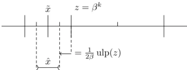
Theorem 1. Let ˆx ∈ R be an approximation to z ∈ R. Let ˜x ∈ Fβ,p be such that ˜x = RN(ˆx). If
|ˆx − z| < 2β1 ulp(z), (7)
then ˜x is a faithful rounding of z.
The condition of Theorem 1 is tight: Assuming β is even, if z = βk, then ˆx = z − 1
2βulp(z) will round to a
value that is not a faithful rounding of z, as illustrated on Figure 1. z = βk ˜x ˆx = 1 2βulp(z)
Figure 1. Tightness of the condition on |ˆx − z|
2.2. Exact residual theorem
When ˜yn is a faithful rounding of a/b, The residual
RN(a − b˜yn) is computed exact. The theorem was first
stated by Markstein [7] and has been more recently proved by John Harrison [5] and Boldo and Daumas [1] using formal provers.
Theorem 2 (Exact residual for the division). Let a, b be two floating-point numbers in Fβ,p, and assume ˜yn is a
faithful rounding of a/b. For any rounding mode ◦, ˜rn+1=
◦(a − b˜yn) is computed exactly (without any rounding),
provided there is no overflow or underflow.
3. Round-to-nearest
In this section, we present several methods to ensure correct rounding. We first present a general method of exclusion intervals that only applies if the quotient a/b is not a midpoint, and how to extend the exclusion intervals
in the case of reciprocal. We then show how to handle the midpoint cases separately.
3.1. Exclusion intervals
A common way of proving correct rounding for a given function in floating-point arithmetic is to study its exclusion intervals (see [5], [8, chap. 8] or [9, chap. 5]).
Given a, b ∈ Fβ,pi, either a/b is a midpoint at precision
po, or there is a certain distance between a/b and the
closest midpoint. Hence, if we assume that a/b is not a midpoint, then for any midpoint m, there exists a small interval centered at m that cannot contain a/b. Those intervals are called the exclusion intervals.
More formally, let us define µpi,po > 0as the smallest
value such that there exist a, b ∈ Fβ,pi and a midpoint m
in precision powith |a/b−m| = βea/b+1µpi,po. If a lower
bound on µpi,po is known, next Theorem 3 can be used to
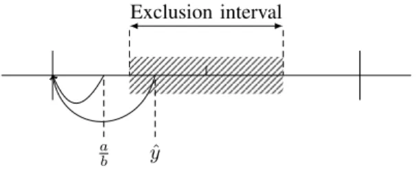
ensure correct rounding, as illustrated by Figure 2 (see [5] or [9, chap. 12] for a proof).
Theorem 3. Let a, b in Fβ,pi be such that a/b is not
midpoint in precision po for the division, and ˆy be in R.
If |ˆy − a/b| < βea/b+1µ
pi,po, then RN(ˆy) = RN(a/b).
To bound the radius of the exclusion intervals, we generalize the method used by Harrison [5] and Marius Cornea [3] to the case of radix β.
Theorem 4. Assuming po≥ 2 and pi≥ 1, a lower bound
on µpi,po is given by
µpi,po ≥
1
2β−pi−po. (8)
Proof: By definition of µpi,po, it can be proved that
a/b is not a midpoint. Let m be the closest midpoint to a/b, and note δβea/b+1 the distance between a/b and m:
a
b = m + δβ
ea/b+1. (9)
By definition, µpi,po is the smallest possible value of
|δ|. As we excluded the case when a/b = m, we have δ �= 0. We write a = Aβ1−pi, b = Bβ1−pi and
m = (M + 1/2)β1−po+ea/b, with A, B, M integers and
βpi−1≤ A, B, M < βpi. Equation (9) becomes
2Bβpoδ = 2Aβpo−1−ea/b− 2BM − B. (10)
Since 2Aβpo−1−ea/b− 2BM − B is an integer and δ �=
0, we have |2Bβpoδ| ≥ 1. Since βpi−1 ≤ B < βpi, the
conclusion follows.
In radix 2, the following example illustrates the sharp-ness of the result of Theorem 4.
Exclusion interval
ˆy
a b
Figure 2. Use of exclusion intervals for prov-ing the correct roundprov-ing
Example 2. In radix 2, for any precision pi = po, b =
1.11 . . . 1 = 2 − 21−pi gives 1 b = 1 2 + 2−1−pi+ 2−1−2pi 1 − 2−pi � �� � δβea/b+1 = 0. 100 . . . 0� �� � pibits 100 . . . 0 � �� � pibits 1 . . .
From this example, an upper bound on µpi,pi can be
deduced, and for any precision pi≥ 1 one has
2−1−2pi ≤ µ
pi,pi ≤
2−1−2pi
1 − 2−pi.
The following result can also be seen as a consequence of Theorem 3 (see [8, chap. 8] or [9, p.163] for a proof). Theorem 5. In binary arithmetic, when pw = po, if ˜x is
a correct rounding of 1/b and ˜y is a faithful rounding of a/b, then an extra Markstein’s iteration yields RNpo(a/b).
3.2. Extending the exclusion intervals
When pw = po = pi, the error bounds of Section 4
might remain larger than the bound on the radius of the exclusion intervals of Section 3.1. A way to prove correct rounding is then by extending the exclusion intervals.
In this subsection, we describe a method to determine all the inputs (a, b) ∈ F2
β,pi such that the quotient a/b is
not a midpoint and lies within a distance βea/b+1µ from
the closest midpoint m. Once all such worst cases are de-termined, correct rounding can be guaranteed considering two cases:
• If a/b corresponds to one of the worst cases, we then
run the Newton-Raphson algorithm on the input (a, b) and check that the result is correct.
• If (a, b) is not one of those worst cases and ˆy is an
ap-proximation to a/b that satisfies |ˆy−a/b| < βea/b+1µ,
then RNβ,po(ˆy) = RNβ,po(a/b).
Unfortunately, there are too many worst cases for the division, but one can apply this method for the reciprocal. Starting from Equation (10) of Section 3.1, one has:
2βpi+po− 2Bβpoδ
� �� �
∆
= B(2M + 1). (11)
Factorizing 2βpi+po − ∆, with |∆| ∈ {1, 2, . . . } into
B(2M + 1) with respect to the range of these integral significands isolates the worst cases. After finding all the worst cases such that |∆| < n, the extended radius is such that µ ≥ β−pi−pon/2. Table 1 shows how many values of
b have to be checked to extend the exclusion interval.
n 2 3 4 5 6 7
binary64 2 68 68 86 86 86
decimal128 1 1 3 3 19 22
Table 1. Number of b to check separately according to the extended radius of the ex-clusion interval µ ≥ β−pi−pon/2
There is a particular worst case that is worth mention-ing: When b = β − 1/2 ulp(β), the correctly rounded reciprocal is 1/β +ulp(1/β), but if the starting point given by the lookup table is not RNβ,pw(1/b), even Markstein’s
iterations cannot give a correct rounding, as shown in Example 3. Example 3. In binary16, (pw= pi= po= 11, β = 2): b = 1.1111111111 ˜x = 0.1 = Table-lookup(b) ˜r = 2−11 (exact) ˜x = 0.1
Hence, ˜x will always equals 0.1, which is not the correct rounding of RN(1/b).
A common method [8] to deal with this case is to tweak the lookup table for this value. If the lookup table is addressed by the first k digits of b, then the output corresponding to the address β − β1−k should be
1/β + β−pw.
3.3. The midpoint case
Theorem 3 can only be used to ensure correct rounding when a/b cannot be a midpoint. In this subsection, we summarize our results about the midpoints for division and reciprocal.
3.3.1. Midpoints in radix 2. Markstein already proved for radix 2 that for any a, b in F2,pi, a/b cannot be a
floating-point number of precision p with p > pi [8]. This means
that a/b cannot be a midpoint in a precision greater or equal to pi. However, Example 4 shows that when pi> po,
a/bcan be a midpoint.
Example 4. Inputs: binary32, output: binary16. a=1.00000001011001010011111 b=1.00101100101000000000000 a/b=0. 11011011001� �� � po=11 1 4 203 ASAP 2010
When computing reciprocals, we have the following. Theorem 6. In radix 2, and for any precisions pi and po,
the reciprocal of a floating-point number in F2,pi cannot
be a midpoint in precision po.
Proof: Given a floating-point number b ∈ F2,pi in
[1, 2), we write b = B21−pi, where B is an integer. If 1/b
is a midpoint in precision po, then 1/b = (2Q + 1)2−po−1
with Q an integer. This gives B(2Q + 1) = 2pi+po. Since
Band Q are integers, this equality can hold only if Q = 0. This implies b = 21+po, which contradicts b ∈ [1, 2).
3.3.2. Midpoints in radix 10. In decimal floating-point arithmetic, the situation is quite different. As in radix 2, there are cases where a/b is a midpoint in precision po, but
they can occur even when pi= po, as shown in Example 5.
Contrarily to the binary case, there are also midpoints for the reciprocal function, characterized by Theorem 7. Example 5. In decimal32 (pi= po= 7, β = 10):
a = 2.000005, b = 2.000000, a/b = 1.000002 5 Theorem 7. In radix 10, for any precisions pi and po,
there are at most two floating-point numbers in a single betade of F10,piwhose reciprocal is a midpoint in precision
po. Their integral significands are B1 = 2pi+po5z1 and
B2= 2pi+po5z2, with z1= � pi− po ln(2) ln(5) − ln(10) ln(5) � , z2= � pi− po ln(2) ln(5) � . Proof of Theorem 7.: Given a floating-point number b∈ F10,piin the betade [1, 10), we rewrite it b = B101−pi.
If 1/b is a midpoint, we then have 1/b = (10Q + 5)10−po−1, with Q ∈ Z, which gives B(2Q + 1) =
2pi+po5pi+po−1. Since 2Q+1 is odd, we know that 2pi+po
divides B. Therefore we have B = 5z2pi+po with z an
integer. Moreover, we know that 1 ≤ b < 10, which gives pi− po ln 2 ln 5 − ln 10 ln 5 ≤z≤ pi− po ln 2 ln 5.
The difference between the two bounds is ln 10/ ln 5 ≈ 1.43. Therefore, there can be at most two integers z between the two bounds.
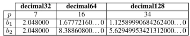
Using Theorem 7, we isolate the at most two values of b whose reciprocal is a midpoint. These values are checked separately when proving the correct rounding of the reciprocal. Table 2 gives the corresponding b when pi= po, for the IEEE 754-2008 decimal formats.
3.4. Correctly handling midpoint cases
Let us recall that the midpoints cases for reciprocal can be handled as explained in §3.3.1 §3.3.2. Hence, we only focus here on division.
decimal32 decimal64 decimal128
p 7 16 34
b1 2.048000 1.67772160. . . 0 1.12589990684262400. . . 0
b2 2.048000 8.38860800. . . 0 5.62949953421312000. . . 0 Table 2. Decimal floating-point numbers whose reciprocal is a midpoint in the same precision
When pi, poand the radix are such that division admits
midpoints, the last Newton-Raphson iteration must be adapted to handle the case where a/b is a midpoint. We propose two methods, depending whether pw= po. Both
methods rely on the exact residual theorem 2 of section 2.2, so it is necessary to use a Markstein iteration (5) for the last iteration.
3.4.1. When pw> po. The exclusion interval theorem of
Section 3.1 does not apply, since there are several cases where a/b is a midpoint in precision po. In that case, we
use the following Theorem 8 instead of Theorem 3. Theorem 8. We assume β is even and pw > po, and we
perform a Markstein iteration:
� ˜r = RN
β,pw(a − b˜y),
˜y� = RN
β,po(˜y + ˜r˜x).
If ˜y is a faithful rounding of a/b in precision pw, and
|ˆy�− a/b| < βea/b+1µ
pi,po, then ˜y� = RNβ,po(a/b).
Proof of theorem 8: If a/b is not a midpoint in precision po, Theorem 3 proves that ˜y� is the correct
rounding of a/b. Now, we assume that a/b is a midpoint in precision po. Since β is even and pw > po, a/b is a
floating-point number in precision pw. Since ˜y is a faithful
rounding of a/b in precision pw, we have ˜y = a/b. Using
Theorem 2, we know that ˜r = 0, which gives ˆy� = a/b,
hence ˜y�= RN
β,po(ˆy�) = RNβ,po(a/b).
Example 6 shows why it is important to round directly in precision po in the last iteration.
Example 6. inputs: binary32, output: binary16. a=1, b = 1.01010011001111000011011 ˜y=0.110000010010111111111111 (faithful) ˜r=1.01010011000111000011011 · 2−24 (exact) ˜y�=0. 11000001001 � �� � 11bits 1000000000000 = RN24(˜y + ˜r˜y) ˜y��=0.11000001010 = RN 11(˜y�)
Due to the double rounding, ˜y�� is not RN 11(a/b).
3.4.2. When pw = po. The quotient a/b cannot be a
midpoint in radix 2. For decimal arithmetic, Example 7 suggests that it is not possible in this case to round correctly using only Markstein’s iterations.
Example 7. In decimal32 (pi= po= pw= 7, β = 10): a = 6.000015, b = 6.000000 ˜x = RN(1/b) = 0.1666667, a/b = 1.000002 5 ˜y0 = RN(a˜x) = 1.000003 ˜r1 = RN(a − b˜y0) =−0.000003 ˜y1 = RN(˜y0+ ˜r1˜x) = 1.000002 ˜r2 = RN(a − b˜y1) = 0.000003 ˜y2 = RN(˜y1+ ˜r2˜x) = 1.000003
Algorithm 1 can be used in this case to determine the correct rounding of a/b from a faithfully rounded approximation.
bs= b ulp(a/b) ; /* bs∈ Fβ,pw */
/* Assume ˜y faithful */
˜r = a − b˜y ; /* ˜r exactly computed. */
if ˜r > 0 then c = RN(2˜r− bs);
if c = 0 then return RN(˜y +1
2 ulp(a/b));
if c < 0 then return ˜y;
if c > 0 then return ˜y + ulp(a/b); else /* ˜r ≤ 0 */
c = RN(2˜r + bs);
if c = 0 then return RN(˜y −1
2 ulp(a/b));
if c < 0 then return ˜y − ulp(a/b); if c > 0 then return ˜y;
end
Algorithm 1: Returning the correct rounding in dec-imal arithmetic when pw= po.
Theorem 9. Let us assume that β = 10 and pw= po and
that ˜y is a faithful rounding of a/b. Then, Algorithm 1 yields the correct rounding of a/b.
Proof: By assumption, ˜y is a faithful rounding of a/b. Thus, there exists � such that − ulp(a/b) < � < ulp(a/b) and ˜y = a/b + �. Also, according to Theorem 2, ˜r = −b�. Six cases, depending on the signs of ˜r and c, have to be considered for the whole proof. We only present here two cases, the others being similar.
• Case ˜r ≥ 0 and 2˜r − b ulp(a/b) < 0: Since ˜r is positive, −� ≤ 0. Moreover, since 2˜r−b ulp(a/b) < 0 we have −1/2 ulp(a/b) < � < 0. Hence, the correct rounding of a/b is ˜y.
• Case ˜r < 0 and 2˜r + b ulp(a/b) = 0: From 2˜r + b ulp(a/b) = 0, we deduce that a/b is a midpoint and RN(a/b) = RN(˜y − 1/2 ulp(a/b)).
4. Error bounds
In this section, we present the techniques we used to bound the error in the approximation to the reciprocal 1/b
or to the quotient a/b obtained after a series of Newton-Raphson iterations. As our aim is to analyze any reasonable sequence combining both Markstein’s or Goldschmidt’s iterations, we only give the basic results needed to analyze one step of these iterations. The analysis of a whole sequence of iterations can be obtained by combining the induction relations proposed here: This is a kind of running error analysis (see [9, chap. 6]) that can be used together with the results of Sections 3.1 and 3.2 to ensure correct rounding.
All the arithmetic operations are assumed to be per-formed at precision pw, which is the precision used for
intermediate computations. Let us denote by � the unit roundoff: In round-to-nearest rounding mode, one has � = 12β1−pw. In the following, we note
ˆ
φn:=|ˆxn− 1/b|, φ˜n:=|˜xn− 1/b|,
ˆ
ψn:=|ˆyn− a/b|, ψ˜n:=|˜yn− a/b|,
˜ρn:=|˜rn− (1 − b˜xn−1)|, ˜σn:=|˜rn− (a − b˜yn−1)|.
4.1. Reciprocal iterations
Both for Markstein’s iteration (3) and for Goldschmidt’s iteration (4), the absolute error ˆφnin the approximation ˆxn
is bounded as ˆ
φn+1≤ ( ˜φn+ |1/b|)˜ρn+1+ |b|˜φ2n, (12)
˜
φn+1≤ (1 + �) ˆφn+1+ |�/b|. (13)
Hence it just remains to obtain induction inequalities for bounding ˜ρn+1.
4.1.1. Reciprocal with the Markstein iteration (3). One has ˜rn+1= RN(1 − b˜xn), hence
˜ρn+1≤ |�||b| ˜φn. (14)
The initial value of the recurrence depends on the lookup-table used for the first approximation to 1/b. Inequal-ity (12) together with (14) can then be used to ensure either faithful or correct rounding for all values of b in [1, β), using Theorems 1 or 3.
At iteration n, if ˜xn is a faithful rounding of 1/b, then
Theorem 2 implies ˜ρn+1= 0. Hence in this case one has
ˆ
φn+1≤ ˜φ2n, which means that no more accuracy
improve-ment can be expected with Newton-Raphson iterations. Moreover, if we exclude the case b = 1, since b belongs to [1, β) by hypothesis, it follows that 1/b is in (β−1, 1).
Since ˜xn is assumed to be a faithful rounding of 1/b, one
has ulp(˜xn) = ulp(1/b), and we deduce
˜
φn+1≤ |b| ˜φ2n+ 1/2 ulp(˜xn), (15)
which gives a sharper error bound on ˜φn+1than (12) when
˜xn is a faithful rounding of 1/b.
6
4.1.2. Reciprocal with the Goldschmidt iteration (4). For the Goldschmidt iteration, one has
˜ρn+1≤ (1 + �)
�
˜ρn+ |b|˜φn−1+ 1
�
˜ρn+ �. (16)
Combining (16) into (13), one can easily deduce a bound on the error ˆφn+1.
4.2. Division iterations
Both for Markstein’s iteration (5) and for Goldschmidt’s iteration (6), one may check that
ˆ
ψn+1≤ |b| ˜ψnφ˜m+ ( ˜φm+ |1/b|)˜σn+1, (17)
˜
ψn+1≤ (1 + �) ˆψn+1+ �|a/b|. (18)
Now let us bound ˜σn+1.
4.2.1. Division with the Markstein iteration (5). In this case, one has
˜σn+1≤ �|b| ˜ψn. (19)
Again, if ˜yn is a faithful rounding of a/b, due to the exact
residual theorem 2, one has ˆψn+1 ≤ |b| ˜ψnφ˜m, which is
the best accuracy improvement that can be expected from one Newton-Raphson iteration.
4.2.2. Division with the Goldschmidt iteration (5). Using the same method as in §4.1.2, we now bound ˜σn+1:
˜σn+1 ≤ (1 + �)(˜σn+ |b| ˜ψn−1)(|b| ˜ψn−1+ |b|˜φm+ ˜σn)
+(1 + �)˜σn+ �|a|. (20)
Then, from (17), a bound on ˆψn+1 can be obtained.
5. Experiments
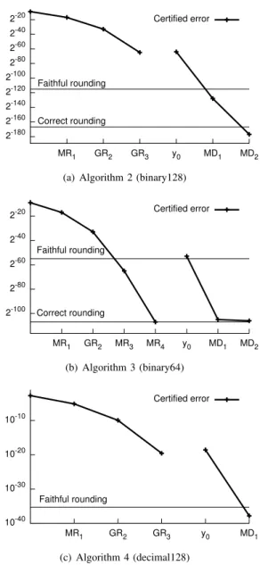
Using the induction relations of Section 4, one can bound the error on the approximations to a/b for a given series of Newton-Raphson iterations, and use it with the sufficient conditions presented in Section 3 to ensure correct rounding. Let us consider three examples : Algorithms 2, 3 and 4 below. The certified error on ˆx and ˆy for those algorithms is displayed on Figure 3.
Algorithm 2 computes the quotient of two binary128 (pi = 113) numbers, the output being correctly rounded
to binary64 (po = 53). The internal format used for
the computations is also binary128 (pw = 113). Since
pi > po, there are midpoints for division, as stated in
Section 3.3. After the MD1 iteration, we know from
Theorem 1 that ˜y is a faithful rounding of a/b, as shown in Figure 3(a). An extra Markstein’s iteration gives an error on ˆy that is smaller than the radius of the exclusion in-terval βea/b+1µ
113,53, as illustrated by Figure 3(a). Hence,
Theorem 8 of Section 3.4.1 applies and guarantees that
˜x = Table-lookup(b); {Error less than 2−8}
˜r = RN113(1 − b˜x); ˜x = RN113(˜x + ˜r˜x); {MR1} | | ˜r = RN113(˜r2); ˜x = RN113(˜x + ˜r˜x); {GR2} | | ˜r = RN113(˜r2); ˜x = RN113(˜x + ˜r˜x); {GR3} ˜y = RN113(a˜x); {y0} ˜r = RN113(a − b˜y); ˜y = RN113(˜y + ˜r˜x); {MD1} ˜r = RN113(a − b˜y); ˜y = RN53(˜y + ˜r˜x); {MD2}
Algorithm 2: Computing the quotient of two bi-nary128 numbers, output in binary64.
˜x = Table-lookup(b); {Error less than 2−8}
˜r = RN53(1 − b˜x); ˜x = RN53(˜x + ˜r˜x); {MR1} | | ˜r = RN53(˜r2); ˜x = RN53(˜x + ˜r˜x); {GR2} ˜r = RN53(1 − b˜x); ˜x = RN53(˜x + ˜r˜x); {MR3} ˜r = RN53(1 − b˜x); ˜x = RN53(˜x + ˜r˜x); {MR4} ˜y = RN53(a˜x); {y0} ˜r = RN53(a − b˜y); ˜y = RN53(˜y + ˜r˜x); {MD1} ˜r = RN53(a − b˜y); ˜y = RN53(˜y + ˜r˜x); {MD2}
Algorithm 3: Computing the quotient of two binary64 numbers, output in binary64.
Algorithm 2 yields a correct rounding of the division, even for the midpoint cases.
Algorithm 3 computes the quotient of two binary64 numbers, with pi= pw= po= 53. Since binary arithmetic
is used and pw= po, there are no midpoints for division.
After the MR4 iteration, ˜x is less than 2 · βe1/b+1µ53,53.
Hence, by excluding two worst cases as explained in Section 3.2, and checking thoses cases, we ensure a correct rounding of the reciprocal using Theorem 3. Since a faithful rounding of a/b at iteration MD1 is ensured by
the error bounds of Section 4, Theorem 5 proves that the next Markstein’s iteration outputs a correct rounding.
Algorithm 4 computes the quotient of two decimal128 numbers, with pi = pw = po = 34. The starting error
given by the lookup table is less than 5 · 10−5. Since
pw = po, Algorithm 1 is needed to ensure the correct
rounding of the division. Notice that to improve the latency, bs in Algorithm 1 can be computed concurrently with the
˜x = Table-lookup(b); | | bs = b ulp(ab); ˜r = RN34(1 − b˜x); ˜x = RN34(˜x + ˜r˜x); {MR1} | | ˜r = RN34(˜r2); ˜x = RN34(˜x + ˜r˜x); {GR2} | | ˜r = RN34(˜r2); ˜x = RN34(˜x + ˜r˜x); {GR3} ˜y = RN34(a˜x); {y0} ˜r = RN34(a − b˜y); ˜y = RN34(˜y + ˜r˜x); {MD1} ˜r = RN34(a − b˜y); Call Algorithm 1.
Algorithm 4: Computing the quotient of two deci-mal128 numbers, output in decideci-mal128.
˜y is a faithful rounding after the MD1 iteration. Hence,
Theorem 9 ensures correct rounding for Algorithm 4.
Conclusion
In this paper, we gave general methods of proving correct rounding for division algorithms based on Newton-Raphson’s iterations, for both binary and decimal arith-metic. Performing the division in decimal arithmetic of two floating-point numbers in the working precision seems to be costly, and we recommend to always use a higher internal precision than the precision of inputs.
We only considered the round-to-nearest rounding mode in this paper. To achieve correct rounding in other rounding modes, only the last iteration of the Newton-Raphson algorithm has to be changed, whereas all the previous computations should be done in the round-to-nearest mode.
References
[1] Sylvie Boldo and Marc Daumas. Representable correcting terms for possibly underflowing floating point operations. In Jean-Claude Bajard and Michael Schulte, editors, Proceedings of the 16th Symposium on Computer Arithmetic, pages 79–86, Santiago de Compostela, Spain, 2003.
[2] Marius Cornea, John Harrison, and Ping Tak Peter Tang. Scientific Computing on Itanium-Based Systems. Intel Press, 2002. [3] Marius Cornea-Hasegan. Proving the IEEE correctness of iterative
floating-point square root, divide, and remainder algorithms. Intel Technology Journal, (Q2):11, 1998.
[4] R. E. Goldschmidt. Applications of division by convergence. Master’s thesis, Dept. of Electrical Engineering, Massachusetts Institute of Technology, Cambridge, MA, USA, June 1964. [5] John Harrison. Formal verification of IA-64 division algorithms. In
M. Aagaard and J. Harrison, editors, Theorem Proving in Higher Order Logics: 13th International Conference, TPHOLs 2000, vol-ume 1869 of Lecture Notes in Computer Science, pages 234–251. Springer-Verlag, 2000.
[6] IEEE Computer Society. IEEE Standard for Floating-Point Arith-metic. IEEE Standard 754-2008, August 2008. available at http://ieeexplore.ieee.org/servlet/opac?punumber=4610933. 2-180 2-160 2-140 2-120 2-100 2-80 2-60 2-40 2-20 MR1 GR2 GR3 y0 MD1 MD2 Correct rounding Faithful rounding Certified error
(a) Algorithm 2 (binary128)
2-100 2-80 2-60 2-40 2-20 MR1 GR2 MR3 MR4 y0 MD1 MD2 Correct rounding Faithful rounding Certified error (b) Algorithm 3 (binary64) 10-40 10-30 10-20 10-10 MR1 GR2 GR3 y0 MD1 Faithful rounding Certified error (c) Algorithm 4 (decimal128)
Figure 3. Absolute error before rounding for each algorithm considered. (M/G: Mark-stein/Goldschmidt, R/D: reciprocal/division)
[7] Peter Markstein. Computation of elementary functions on the IBM RISC System/6000 processor. IBM J. Res. Dev., 34(1):111–119, 1990.
[8] Peter Markstein. IA-64 and elementary functions: speed and precision. Hewlett-Packard professional books. 2000.
[9] Jean-Michel Muller, Nicolas Brisebarre, Florent de Dinechin, Claude-Pierre Jeannerod, Vincent Lef`evre, Guillaume Melquiond, Nathalie Revol, Damien Stehl´e, and Serge Torres. Handbook of Floating-Point Arithmetic. Birkh¨auser Boston, 2010. ACM G.1.0; G.1.2; G.4; B.2.0; B.2.4; F.2.1., ISBN 978-0-8176-4704-9. [10] Siegfried M. Rump, Takeshi Ogita, and Shin’ichi Oishi. Accurate
floating-point summation part I: Faithful rounding. SIAM Journal on Scientific Computing, 31(1):189–224, 2008.
[11] Liang-Kai Wang and Michael J. Schulte. A decimal floating-point divider using Newton-Raphson iteration. J. VLSI Signal Process. Syst., 49(1):3–18, 2007.