HAL Id: hal-00703674
https://hal.archives-ouvertes.fr/hal-00703674
Submitted on 4 Jun 2012HAL is a multi-disciplinary open access archive for the deposit and dissemination of sci-entific research documents, whether they are pub-lished or not. The documents may come from teaching and research institutions in France or abroad, or from public or private research centers.
L’archive ouverte pluridisciplinaire HAL, est destinée au dépôt et à la diffusion de documents scientifiques de niveau recherche, publiés ou non, émanant des établissements d’enseignement et de recherche français ou étrangers, des laboratoires publics ou privés.
Layering and wetting transitions for an interface model
Salvador Miracle-Sole
To cite this version:
Salvador Miracle-Sole. Layering and wetting transitions for an interface model. 11th Granada Seminar, 2010, La Herradura (Granada), Spain. pp.190-194. �hal-00703674�
for an interface model
Salvador Miracle Sol´e
Centre de Physique Th´eorique, CNRS, Marseille, France
Abstract
We study the solid-on-solid interface model above a horizontal wall in three dimensional space, with an attractive interaction when the interface is in contact with the wall, at low temperatures. The system presents a sequence of layering transitions, whose levels increase with the temperature, before the complete wetting above a certain value of this quantity.
Published in Non-Equilibrium Statistical Physics Today, 11th Gra-nada Seminar, P.L. Garrido, J. Marro, F. de los Santos (Eds.), AIP Conference Proceedings, no. 1332, pp. 190–194 (ISBN 978-0-7354-0887-6), American Institute of Physics, Melville, NY, 2011.
Keywords: SOS model, wetting and layering transitions, interfaces, entropic repulsion. Classification: 68.08.Bc, 05.50.+q, 60.30.Hn, 02.50.-r
Consider the square lattice Z2. To each site x = (x1, x2) of the lattice,
an integer variable φx ≥ 0 is associated which represents the height of the
interface at this site. The system is first considered in a finite box Λ ⊂ Z2
with fixed values of the heights outside. Each interface configuration on Λ: {φx}, x ∈ Λ, denoted φΛ, has an energy defined by the Hamiltonian
HΛ(φΛ| ¯φ) = 2J X hx,x′i∩Λ6=∅ |φx− φx′| − 2(J − K) X x∈Λ δ(φx) + 2J|Λ|, (1)
where J and K are positive constants, the function δ equals 1, when φx = 0,
and 0, otherwise, and |Λ| is the number of sites in Λ. The first sum is taken 1
S. Miracle Sol´e / Layering and wetting transitions 2 over all nearest neighbors pairs hx, x′i ⊂ Z2, such that at least one of the
sites belongs to Λ, and one takes φx = ¯φx when x 6∈ Λ, the configuration ¯φ
being the boundary condition, assumed to be uniformly bounded.
In the space R3, the region obtained as the union of all unit cubes centered
at the sites of the lattice Λ × Z, that satisfy x3 ≤ φ(x1, x2), is supposed to be
occupied by fluid +, while the complementary region above it, is occupied by fluid −. The common boundary between these regions is a surface in R3, the
microscopic interface. The region x3 ≤ −1/2 is considered as the substrate,
also called the wall W .
The considered system differs from the usual SOS model by the restriction to non-negative height variables and the introduction of the second sum in the Hamiltonian, the term describing the interaction with the substrate.
The probability of the configuration φΛ, at the inverse temperature β =
1/kT , is given by the finite volume Gibbs measure
µΛ(φΛ| ¯φ) = Z(Λ, ¯φ)−1exp ( − βHΛ(φΛ| ¯φ)), (2)
where Z(Λ, ¯φ) is the partition function Z(Λ, ¯φ) =X
φΛ
exp ( − βHΛ(φΛ | ¯φ)). (3)
Local properties at equilibrium can be described by correlation functions between the heights on finite sets of sites, obtained as expectations with respect to the Gibbs measure.
We next briefly describe some general results, which are an adaptation to our case of analogous results established by Fr¨ohlich and Pfister (ref. [1]) for the semi-infinite Ising model.
Let Λ ⊂ Z2 be a rectangular box of sides parallel to the axes. Consider
the boundary condition ¯φx = 0, for all x 6∈ Λ, and write Z(Λ, 0) for the
corresponding partition function. The associated free energy per site, τW − = − lim
Λ→∞(1/β|Λ|) ln Z(Λ, 0), (4)
represents the surface tension between the medium − and the substrate W . This limit (4) exists and 0 ≤ τW − ≤ 2J. One can introduce the densities
ρz = lim Λ→∞ z X z′=0 hδ(φx− z′)i(0)Λ , ρ0 = lim Λ→∞hδ(φx)i (0) Λ , (5)
Their connection with the surface free energy is given by the formula τW −(β, K) = τW −(β, 0) + 2
Z K
0 ρ0(β, K
′)dK′. (6)
The surface tension τW+
between the fluid + and the substrate is τW+
= 0. In order to define the surface tension τ+− associated to a horizontal
inter-face between the fluids + and − we consider the ordinary SOS model, with boundary condition ¯φx = 0. The corresponding free energy gives τ+−. With
the above definitions, we have τW+
(β) + τ+−(β) ≥ τW −(β, K). (7)
and the right hand side in (7) is a monotone increasing and concave (and hence continuous) function of the parameter K. This follows from relation (6) where the integrand is a positive decreasing function of K. Moreover, when K ≥ J equality is satisfied in (7).
In the thermodynamic description of wetting, the partial wetting situation is characterized by the strict inequality in equation (7), which can occur only if K < J, as assumed henceforth. We must have then ρ0 > 0. The
complete wetting situation is characterized by the equality in (7). If this occurs for some K, say K′ < J, then equation (6) tells us that this condition
is equivalent to ρ0 = 0. Then, both conditions, the equality and ρ0 = 0, hold
for any value of K in the interval (K′, J).
On the other hand, we know that ρ0 = 0 implies also that ρz = 0, for any
positive integer z. This indicates that, in the limit Λ → ∞, we are in the + phase of the system, although we have used the zero boundary condition, so that the medium − cannot reach anymore the wall. This means also that the Gibbs state of the SOS model does not exist in this case.
That such a situation of complete wetting is present for some values of the parameters does not follow, however, from the above results. Actually this fact, as far as we know, remains an open problem for the semi-infinite Ising model in 3 dimensions. For the model we are considering an answer to this problem has been given by Chalker [2].
Chalker’s result. We use the following notation:
u = 2β(J − K), t = e−4βJ. (8)
If u < − ln(1 − t2), then ρ 0 = 0.
S. Miracle Sol´e / Layering and wetting transitions 4 Thus, for any given values of J and K, there is a temperature below which the interface is almost surely bound and another higher one, above which it is almost surely unbound and complete wetting occurs. At low temperature (i.e., if u > ln 16), we have ρ0 > 0.
The object of our study is to investigate the region not covered by these results when the temperature is low enough. As mentioned in the abstract, we shall prove that a sequence of layering transitions occurs before the system attains complete wetting. More precisely the main results can be summarized as follows.
Theorem 1. Let the integer n ≥ 0 be given. For any ǫ > 0 there exists a value t0(n, ǫ) > 0 such that, if the parameters t, u, satisfy 0 < t < t0(n, ǫ)
and
− ln(1 − t2) + (2 + ǫ)tn+3 < u < − ln(1 − t2) + (2 − ǫ)tn+2, (9)
then the following statements hold: (1) The free energy τW − is an analytic
function of the parameters t, u. (2) There is a unique Gibbs state µn, a
pure phase associated to the level n. (3) The density is ρ0 > 0. The second
inequality in (9) is not needed in the case n = 0.
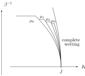
An illustration for this theorem, in the plane (K, β−1), is given in Figure
1. From it we can see, as mentioned in the abstract, that if the parameter K is kept fixed, that seems natural since it depends on the properties of the substrate, then the value n of the level increases when the temperature is increased.
Concerning this theorem, the following remarks can be made:
(1) The analyticity of the free energy comes from the existence of a con-vergent cluster expansion for this system. This implies the analyticity, in a direct way, of some correlation functions and, in particular, of the density ρ0.
(2) The unicity of the Gibbs state means that the correlation functions converge, when Λ → ∞, to a limit that does not depend on the chosen (uniformly bounded) boundary condition ¯φx. Being unique and translation
invariant this state represents a pure phase. It is associated to a level n in the sense that, for the typical configurations of the state, large portions of the interface are near to the level n.
(3) The condition ρ0 > 0 means that the interface remains at a finite
distance from the wall and hence, we have partial wetting. We can see that the region where this condition holds is, according to the Theorem, much
larger, at low temperatures, than the region initially proved by Chalker. It comes very close to the line above which it is known that complete wetting occurs.
(4) We have, t0(n, ǫ) → 0 when n → ∞ or ǫ → 0.
The reason why t0(n, ǫ) depends on ǫ, satisfying remark 4, has an
expla-nation. One may believe that the regions of uniqueness of the state extend in such a way that two neighboring regions, say those corresponding to the levels n and n + 1, will have a common boundary where the two states µn
and µn+1 coexist. µ0 µ1 µ2 µ3 ✻ ✲ β−1 K J wetting complete
FIGURE 1. The analyticity regions of Theorem 1.
At this boundary there will be a first order phase transition, since the two Gibbs states are different. The curve of coexistence does not exactly coincide with the curve u = − ln(1 − t2) + 2tn+3. Theorem 1 says that it is
however very near to it, if the temperature is sufficiently low.
Let us formulate in the following statement the kind of theorem that we expect. We think that such a statement could be proved using, as for Theorem 1, an extension of the Pirogov-Sinai theory.
Statement. For each given integer n ≥ 0, there exists t0(n) > 0 and a
S. Miracle Sol´e / Layering and wetting transitions 6
the statements of Theorem 1 hold, for t in this interval, in the region where
ψn+1(t) < u < ψn+2(t) and for n = 0, in the region ψ1(t) < u. When
u = ψn+1(t) the two Gibbs states, µn and µn+1, coexist.
The existence of a sequence of layering transitions has been proved for a related model, known as the SOS model with an external magnetic field. See the works by Dinaburg, Mazel [3], Cesi, Martinelli [4] and Lebowitz, Mazel [5]. This model has the same set of configurations as the model considered here, but a different energy: The second term in (1) has to be replaced by the term +hPx∈Λφx to obtain the Hamiltonian of the model with an external
magnetic field. The method followed for the proof of the Theorem is essen-tially analogous to the method developed for the study of that model. The most important difference between the two systems concerns the restricted ensembles and the computation of the associated free energies.
Concerning the proof of Theorem 1 (paper in preparation) let us say that, for an interesting class of systems, among which our model is included, one needs some extension of the Pirogov-Sinai theory of phase transitions (see ref. [6]). In such an extension certain states, called the restricted ensembles, play the role of the ground states in the usual theory. They can be defined as a Gibbs probability measure on certain subsets of configurations. In the present case one considers, for each n = 0, 1, 2, . . ., subsets of configurations which are in some sense near to the constant configurations φx= n.
Namely, we consider the set Cres
k (Λ, n) of the microscopic interfaces, with
boundary at height ¯φx = n, and whose Dobrushin walls have, all of them,
horizontal projections with diameter less than 3k + 3 (these walls are the maximally connected sets of vertical plaquettes of the interface). The Gibbs measure defined on the subset Cres
k (Λ, n) is the restricted ensemble
corre-sponding to the level n. The associated free energies per unit area fk(n) = − lim
Λ→∞(1/β|Λ|) ln
X
φΛ∈Cresk (Λ,n)
exp(−βH(φΛ|n)) (10)
can be computed, with the help of cluster expansions (see, for instance, ref. [7]), as a convergent power series in the variable t. Then one is able to study the phase diagram of the restricted ensembles. The restricted ensemble at level n is said to be dominant, or stable, for some given values of the parameters u and t, if fk(n) = minn′fk(n′). We then have:
a, b ≥ 0 be two real numbers. Let 0 < t ≤ t1(k) = (3k + 3)−4. If
− ln(1 − t2) + (2 + a)tn+3 ≤ u ≤ − ln(1 − t2) + (2 − b)tn+2, (11)
then, we have
fk(n) ≤ fk(h) − at3n+3+ O(t3n+4), for any h ≥ n + 1, (12)
fk(n) ≤ fk(h) − bt3n+ O(t3n+1), for any 0 ≤ h ≤ n − 1. (13)
We notice that k ≥ n is the useful case in the proof of Theorem 1, and that the remainders in inequalities (12) and (13) can be bounded uniformly in h. Then the proof of Theorem 1 consists in showing that the phase diagram of the pure phases at low temperature is close to the phase diagram of the dominant restricted ensembles.
References
[1] J. Fr¨ohlich, C.E. Pfister, Semi-infinite Ising model: I, II, Commun. Math. Phys. 109, 493–523 (1987) and 112, 51–74 (1987)
[2] J.T. Chalker, The pinning of an interface by a planar defect, J. Phys. A: Math. Gen. 15, L481–L485 (1982)
[3] E.I. Dinaburg, A.E. Mazel, Layering transition in SOS model with
exter-nal magnetic field, J. Stat. Phys. 74, 533–563 (1996)
[4] F. Cesi, F. Martinelli, On the layering transition of an SOS interface
interacting with a wall: I, Equilibrium results, J. Stat. Phys. 82, 823–913
(1996)
[5] J.L. Lebowitz, A.E. Mazel, A remark on the low temperature behavior of
an SOS interface in half space, J. Stat. Phys. 84, 379–397 (1996)
[6] Ya. G. Sinai, Theory of Phase Transitions: Rigorous Results, Pergamon Press, Oxford, 1982
[7] S. Miracle-Sole, On the convergence of cluster expansions, Physica A 279, 244–249 (2000)