Design of an Incentive-based Demand Side
Management Strategy for Stand-Alone Microgrids
Planning
Juan Carlos Oviedo Cepedaa∗, Arash Khalatbarisoltanib, Loïc Boulonb, German Alfonso Osma-Pintoa, Cesar Antonio Duarte Gualdrona and Javier Enrique Solano Martineza
aDepartment of Electrical Engineering, Universidad Industrial de Santander, Calle 9 - Carrera 27,
680002, Bucaramanga, Santander, Colombia.
bDepartment of Electrical Engineering, Université du Québec à Trois-Rivières, 3351 Boulevard des
Forges, G8Z 4M3, Trois-Rivières, Quebec, Canada.
Abstract—Demand Side Management Strategies (DSMSs) can play a significant role in reducing installation and operational costs, Levelized Cost of Energy (LCOE), and enhance renewable energy utilization in Stand-Alone Microgrids (SAMGs). Despite this, there is a paucity in literature exploring how DSMS affects the planning of SAMGs. This paper presents a methodology to design an incentive-based DSMS and evaluate its impact on the planning phase of a SAMG. The DSMS offers two kinds of incentives, a discount in the flat tariff to increase the electrical energy consumption of the users, and an extra payment added to the fare to penalize it. The design of the methodology integrates the optimal energy dispatch of the energy sources, the tariff design, and its sizing. In this regard, the main contribution of this paper is the design of an incentive-based DSMS using a Disciplined Convex approach, and the evaluation of its potential impacts over the planning of SAMG. The methodology also computes how the profits of the investors are modified when the economic incentives vary. A study case shows that the designed DSMS effectively reduces the size of the energy sources, the LCOE, and the payments of the customers for the purchased energy.
Key words—Stand-Alone Microgrids, Planning, Sizing, Energy Management, Demand-Side Management.
1. Introduction
The access to affordable and high-quality electricity service is considered as one of the barriers to overcome in order to achieve sustainable economic and social development in rural areas [1]. The installation of stand-alone microgrids (SAMG), when the extension of the utility grid is not feasible, is the most common alternative for rural electrification [2]–[6]. SAMG projects are gen-erally considered as a good solution to provide electric
energy services to isolated communities [7]. However, SAMG face technical and financial challenges that need to be addressed in their planning.
The technical aspects of the planning of SAMG refer to the sizing and the design of an appropriate Energy Management Strategy (EMS). The EMS must consider the uncertainties introduced by the Renewable Energy Resources (RERs) [8, 9]. One of the ways to deal with the uncertainties is the addition of Demand Side Management Strategies (DSMSs) to the EMS. Sending a signal to the customers to increase or decrease the consumption can reduce the risk of excess and lack of energy introduced by the RERs. Additionally, DSMSs can reduce operational costs, harmful environmental emissions, and increase the reliability of the microgrid [10]–[12].
The DSMS can affect the patterns of consumption of the customers using direct or indirect strategies [13]. One of the advantages of indirect DSMS is the possibility of the customers to choose either to participate or not in the program [14]. Indirect DSMS include pricing programs, incentive programs, rebates, subsidies, and education programs. Incentive programs offer economic incentives to the customers either to reduce or to increase the electrical energy consumption [15, 16]. Adequately designed incentives can reflect electricity production costs, which can motivate the customers to shift their demand when it is more convenient to produce electricity [17]. Additionally, adequately designed incentives can lead to energy conservation, and therefore, are desired when the energy generation is limited [18].
Palma-Behnke et al. introduce a DSMS for the op-eration of a microgrid based on sending information to the customers about the availability of electric energy
TABLE I: Variable declaration SAMG modeling
t Hour of optimization Hours
T Total number of hours to optimize Hours
n Specific customer in the microgrid Unitless
m Specific generator or storage system of the
microgrid
Unitless
M Total number of generators and storage
systems of the microgrid
Unitless
Do,t Initial Electrical demand of the community kWh
Dt Final Electrical demand of the community kWh
Dno,t Initial Electrical demand of the n customer kWh
Dn
t Final Electrical demand of the n customer kWh
ent Self-elasticity of the n customer Unitless
Im Unitary initial investment of the m device USD/kW
Cm Installed capacity of the m device kW, kWh
Em Quantity of energy delivered with the m
device
kWh
EB,t Stored energy in the Battery at time t kWh
λm Unitary costs of generation of the m
de-vice
USD/kWh
ξm Unitary maintenance costs of the m device USD/kWh
LP SP Loss of Power Supply Probability Unitless
EP SP Excess of Power Supply Probability Unitless
CAPEX Capital Expenditures USD
OPEX Operational Expenditures USD
Financial analysis
ζ Total capital expenditures USD
ϑ Total operational expenditures USD
ϕci Percentage of the CAPEX paid by the
investor
Unitless
ϕcg Percentage of the CAPEX paid by the
government
Unitless
ϕoi Percentage of the OPEX paid by the
in-vestor
Unitless
ϕog Percentage of the OPEX paid by the
gov-ernment
Unitless
ϕpr Percentage of the profits to pay the
incen-tives
Unitless
R Internal Rate of Return for the investors Unitless
Fc Electric energy conservation factor Unitless
Incentive-based DSMS design
πt Vector of prices of the incentive-based
tariff
USD/kWh
πmin Minimum value of the incentive USD/kWh
πmax Maximum value of the incentive USD/kWh
πf lat Original price of the tariff without DSMS USD/kWh
πf Flat price of the tariff USD/kWh
πi,t Price of the incentive at t hour USD/kWh
ψL Diesel price per liter USD/liter
Γninc Payments of the n customer under the
designed tariff
USD
Study case
CDG Installed capacity of diesel generator kW
CP V Installed capacity of photovoltaic
genera-tion
kW
CB Installed capacity of Battery kWh
IDG Unitary investment costs of diesel
genera-tor
USD/kW
IP V Unitary investment costs of photovoltaic
generation
USD/kW
IB Unitary investment costs of Battery USD/kWh
ξDG Unitary maintenance costs of the diesel
generator
USD/kWh
ξP V Unitary maintenance costs of the
photo-voltaic system
USD/kW
ξB Unitary maintenance costs of the battery USD/kW
EDG,t Amount of energy delivered with the diesel
generator
kWh
FDG,t Fuel consumption of the diesel generator kWh
EP V,t Amount of energy delivered with the
pho-tovoltaic generation
kWh
EEE,t Amount of energy in excess kWh
ELE,t Lack of energy to fulfill the demand kWh
NP V Number of photovoltaic panels Unitless
ρP V Derating factor of the photovoltaic system Unitless
α, β, γ Parameters to compute fuel consumption Unitless
PST C Output power of one PV module under
standard conditions
kW
GA,t Global solar radiation on the surface of the
PV array
W/m2
GST C Global solar radiation at standard
condi-tions
W/m2
CT Temperature coefficient of the PV modules %/◦C
TC,t Working temperature of the PV cells ◦C
TA,t Ambient temperature near to the PV cells ◦C
TST C Temperature of the PV cells at standard
conditions
◦
C GN OCT solar radiation at NOCT conditions W/m2
TN OCT Working temperature of the PV cells at
NOCT conditions
◦
C Ta,t,N OCT Ambient temperature at NOCT conditions ◦C
[19]. Lighting red, yellow, or green LEDs, they inform the customers to make a significant reduction, medium reduction or keep the current electrical consumption, respectively. The signals are communicated several hours in advance. The authors did not design any economic incentive or punishment to incentivize consumers to participate.
Mazidi et al. introduce a DSMS to improve the reserve capacity of a microgrid and minimize opera-tional costs [20]. Using responsive loads and distributed generation units, they create the reserve requirement for compensating renewable forecast errors. Residential,
commercial, and industrial customers can participate in the program either to reduce energy consumption or to schedule reserve capacity. Agbayani et al. propose a stochastic programming model to minimize operating costs and emissions in a smart microgrid with renewable sources [21]. The authors formulate a DSMS to reduce the uncertainties introduced by RERs using incentive-based payments. Residential, commercial, and industrial customers can participate in the DSMS.
Chenye et al. use dynamic potential game theory to tackle the intermittent nature of wind power generation on a SAMG [22]. The authors formulate a decentralized
DSMS to reduce operational costs. Additionally, a char-acterization of the self-interests of the end-users helps to build the best strategies of the formulated game model. Simulation results with field data show a reduction of 38% of the operational costs compared to a benchmark where no DSMSs was applied.
References [19]–[22] show the benefits of using DSMSs in the operational phase of a microgrid. How-ever, they do not consider the potential effect of applying a DSMS in the planning phase of a microgrid project. The Integrated Resource Planning (IRP) framework mea-sures the benefits of implementing a DSMS in the planning phase of microgrids . [23, 24]. Zhu et al. use a similar approach to evaluate the impact of load control, interruptible loads, and shiftable loads over the design of a microgrid in Shanghai, China [25, 26]. The study shows that using DSMSs, it is possible to reduce the size of the facilities of the microgrid, decrease invest-ments, and reduce social costs. Kahrobaee et al. consider dynamic tariffs in the sizing of Wind-turbine/Battery Energy Storage System (BESS) for a house [27]. The authors combine a rule-based controller, a Monte Carlo approach, and a Particle Swarm Optimization (PSO) to perform the sizing of the components. However, the com-bination of multiple steps of different types and the lack of an optimization formulation for energy management can lead to sub-optimal results. Erdinc et al. aim to improve these drawbacks by providing a Mixed Integer Linear Programming (MILP) formulation to design the optimal energy management strategy [28]. The work considers a Real-Time Pricing tariff scheme. However, this work did not consider how to design the DSMS itself and how different DSMSs will impact the sizing of the energy sources.
Nojavan et al. propose a Mixed-Integer Non-Linear Programming (MINLP) formulation for the sizing of a MG considering a tariff-based DSMSs [29]. However, the authors assume that 20% of the load reacts to a Time of Use (ToU) tariff ignoring the effects of the self-elasticity of the demand. Majidi et al. use Monte Carlo to determine the size of a BESS in a MG [30]. However, similarly to [29], the authors did not consider how the customers react to the DSMS; they assume that 20% of the load will react to a ToU tariff. Mehra et al. propose a work to measure the economic value of applying DSMS in the sizing of a nanogrid [31,32]. Nevertheless, the work considers the effects of only one kind of DSMS and over a small size grid. Kumar et al. Analyze the techno-economic viability of a rural grid connected microgrid considering a demand response strategy using Homer software [33]. The study shows the feasibility of applying the demand response strategy reducing the
Levelized Cost of Energy (LCOE). However, the study does not use an optimal energy dispatch strategy, neither an optimal tariff for the demand response strategy, which can lead to sub-optimal solutions.
Despite that literature has shown that applying DSMSs in microgrids planning reduces the total costs of the project, the studies found by the authors present some drawbacks that can be improved. The first drawback is that some works combine different methods to im-plement the EMS, DSMS, and sizing, which can lead to sub-optimal results. The second drawback is the tendency of the works to ignore the effect of the self-elasticity of the customers when the planner applies a tariff-based DSMS. A third drawback is that the authors do not focus on the design of the DSMS itself. In this regard, the present work aims to fulfill the gaps found in the literature by providing a methodology that uses one single formulation for the planning of SAMG considering the application of an incentive-based DSMS. The proposed methodology considers the self-elasticity of the customers to compute their responses to the tariffs. Additionally, the methodology designs the DSMS itself and evaluate its impact on SAMGs planning. A summary of the contributions of the methodology to the state of art proceed as follows:
• Design a methodology to obtain the optimal sizing, the optimal energy dispatch strategy, and the opti-mal economic incentives to guarantee the financial viability of a SAMG project using a Disciplined Convex formulation.
• Evaluate the impact of the economic incentives for the customers over the sizing, energy management, and fuel consumption of a SAMG project.
• Compare the results of the proposed method against a scenario without DSMS under a sensitive analysis that considers variations in the solar radiation, the fuel price, and the price of the storage system. The description of the rest of the article proceeds as follows: Section2presents the definition of the problem and the proposed solution. Section 3 presents a study case as an example of the application of the method-ology. Section 4 presents the results of the simulations. Finally, Section 5 presents the conclusions and future direction.
2. Problem formulation and proposed solution The considered problem is the design of an economic incentive-based DSMS and the evaluation of their poten-tial impact over the sizing of a SAMG. In this matter, solving two problems is required: sizing and energy management. On one side, the sizing must define the
capacity of each of the energy sources of the SAMG. In this process, it is highly desirable to increase reliability while minimizing investment costs, output energy costs, or fuel consumption, among others [34,35]. On the other side, the DSMS is in charge of doing the economic dispatch for the microgrid. The DSMS includes the monetary incentives or punishments for the customers to increase or reduce the consumption, respectively.
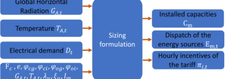
The methodology uses a Disciplined Convex formu-lation that integrates economic incentives as indirect de-mand response mechanisms. The methodology assumes that the planner knows historic weather variables and electrical demand data over the optimization horizon. Moreover, the methodology assumes that the planner can know the price elasticity of the demand of the customers and that the customers will change their patterns of consumption to minimize their payments. The formulation uses the initial demand Do and final
demand Df notations to make a difference between the
demand without economic incentives and the demand with economic incentives. Figure1shows the inputs and outputs of the proposed methodology.
Global Horizontal Radiation 𝐺𝐴,𝑡 Temperature 𝑇𝐴,𝑡 Electrical demand 𝐷𝑡 Sizing formulation Installed capacities Cm F𝑐, 𝑒, 𝜑𝑐𝑔, 𝜑𝑐𝑖, 𝜑𝑜𝑔, 𝜑𝑜𝑖, 𝐺𝐴,𝑡, 𝑇𝐴,𝑡, 𝜆𝑢, 𝜉𝑢, 𝐼𝑚 Dispatch of the energy sources Em,t Hourly incentives of the tariff 𝜋𝑖,𝑡
Figure 1: Flowchart for the methodology.
2.1. Proposed solution
The proposed solution considers the possibility of having public funding for the SAMG. The following equations use ϕcg, ϕci, ϕog and ϕoi to measure the
impact of the subsidies offered by the government for the Capital Expenditures and Operational Expenditures of the SAMG project according to Eqs. (1) and (2).
ϕci+ ϕcg = 1 (1)
ϕoi+ ϕog = 1 (2)
The aim of the methodology is to minimize the Capital Expenditures (CAPEX=ζ) and the Operational Expenditures (OPEX=ϑ) that the government need to pay for the SAMG project.
min ϕcgζ + ϕogϑ (3)
Where ζ and ϑ are shown by Eqs. (4) and (5)
respectively. ζ = M X m=1 CmIm (4) ϑ = T X t=1 M X m=1 (λm,t+ ξm,t)Em,t (5)
The proposed formulation considers the energy prices as the only revenue stream for the investors. In this regard, they must be enough to guarantee the recovery of their investments and the expected Internal Rate of Return (R ∈ (0, 1)). Eq. (6) guarantees that the investors recover their investment and the value of R for the worst-case scenario. −(ϕciζ + ϕoiϑ)(1 + R) + T X t=1 Dtπt≥ 0 (6)
Eq. (7) introduces an energy conservation factor Fc ∈
(0, ∞). Fc defines how the electric energy
consump-tion will be modified after the implementaconsump-tion of the incentive-based tariff πt. If Fc= 1, the sum of the final
demand is the same as the sum of the original demand.
T X t=1 Dt− Fc T X t=1 Do,t= 0 (7)
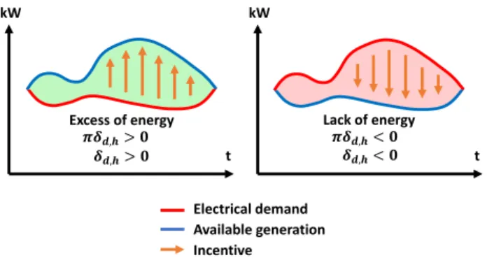
The designed DSMS encourages energy consumption offering a discount to the flat tariff. To discourage energy consumption, the DSMS charges an extra price to the flat tariff. To define the economic value of the incentive, the investors need to estimate how much money they can offer and how much money they can charge to the customers as an extra fare. If the incentives are paid by the investors to increase the electric energy consumption, the profit of the investors reduces. On the other side, if the incentives are paid to the investors to reduce electric energy consumption, the profit of the investors will increase. Figure 2 illustrates the two scenarios.
The design of the incentives requires two different prices πf and πt. πf is a decision variable of one
dimension, πtis a decision variable of dimension T . The
final tariff πt charges the customers with the sum of πf
and πt as described by Eq. (8).
πt= πf + πi,t (8)
In Eq. (9) Dtnrepresents the electric energy
consump-tion of the customer n and time t. Eq. (9) multiply the electric energy consumption with the price of the energy
Electrical demand Available generation Incentive kW t kW t Lack of energy 𝜹𝒅,𝒉< 𝟎 Excess of energy 𝜹𝒅,𝒉> 𝟎 𝝅𝜹𝒅,𝒉> 𝟎 𝝅𝜹𝒅,𝒉< 𝟎
Figure 2: Possible scenarios for the economic incentive of the DSMS.
πt, to obtain the payments of the n customer using the
incentive-based tariff. Eq. (10) set a limit to the values that the planner offers as incentives.
Γninc= T X t=1 Dtnπt (9) πmin≤ πt≤ πmax (10)
The planners can also define the amount of money that they want to use to pay the economic incentives. Eq. (11) defines a restriction to guarantee that the total payments of incentives do not overpass a predefined percentage (ϕpr) of the profits. T X t=1 πt≤ ϕpr T X t=1 Dtπt− (ϕciζ + ϕoiϑ) ! (11) The planners will need not only to know how much money to pay or charge, but also they will need to know how much the customers will modify their patterns of consumption in the presence of the stimulus. Different approaches are being considered by researchers to solve this problem. Considering the customers’ response to the price signal and the profit of the system operator (SO), the authors maximize customers and SO utility in [36]. The research presented in [37] formulates a methodology to estimate the optimal real-time price signal, considering how the customers will respond to it. On another side, [38] proposes to use self-elasticity and cross elasticity of each user to estimate how cus-tomers will react to an Emergency Demand Response Program and a Time of Use tariff. Here, the proposed methodology uses a concept from microeconomics that relates the price of the goods with its consumption [39]. This concept allows predicting how customers will react to different price incentives [38, 40].
ent = πt(D n t − Dno,t) Do,tn (πf lat− πt) (12) 3. Study case
The study case aims to illustrate the capabilities and performance of the proposed methodology. To do so, the sizing and the design of an incentive-based DSMS operate over a hypothetical SAMG located at longi-tude 770160800 West and latitude 504103600 North (Nuquí, Colombia). The microgrid is composed of Photovoltaic panels (PV), a BESS, a Diesel Generator (DG) and a Demand Response (DR) system. TableIIsummarizes the unitary costs obtained from the local providers and used for the simulations. TableIIdescribes the maintenance as the yearly costs of the installed capacities of the energy sources per kW or kWh.
TABLE II: Unitary system costs for simulations.
System Initial Investment Maintenance (year) Operation
PV 1,300 U SD/kW 0.02 U SD/kW 0 USD
BESS 420 U SD/kW h 0.01 U SD/kW h 0 USD
DG 550 U SD/kW 0.75 U SD/kW h Eq.27
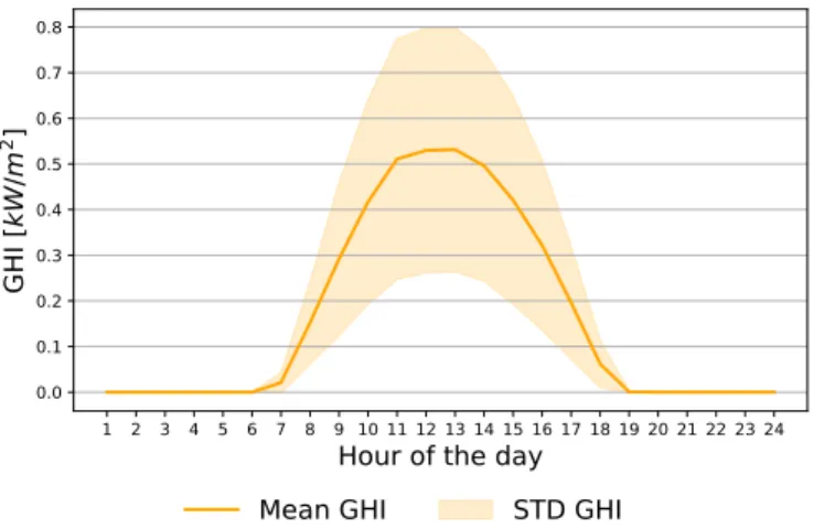
Due to the lack of a historical electrical demand of the community, we propose here to generate a typical community profile using the synthetic load profile gener-ator of the Homer Pro software. The standard community profile is scaled up to make it coincide with the reported average peak in Nuquí [41]. Meteonorm database of PvSyst software provides the Global Horizontal Radi-ation (GHI) and temperature. Figure 3 show the daily average load profile, Figure 4 shows the daily average GHI, and Figure 5shows daily average the temperature.
1 2 3 4 5 6 7 8 9 10 11 12 13 14 15 16 17 18 19 20 21 22 23 24
Hour of the day
50 100 150 200 250 300 350
Global Horizontal Radiation [
kW
/m
2
]
Mean demand
STD demand
1 2 3 4 5 6 7 8 9 10 11 12 13 14 15 16 17 18 19 20 21 22 23 24
Hour of the day
0.0 0.1 0.2 0.3 0.4 0.5 0.6 0.7 0.8
GHI [
kW
/m
2]
Mean GHI
STD GHI
Figure 4: Daily average Global Horizontal Radiation
1 2 3 4 5 6 7 8 9 10 11 12 13 14 15 16 17 18 19 20 21 22 23 24
Hour of the day
20 22 24 26 28 30
Temperature [
C]
Mean temperature
STD temperature
Figure 5: Daily average temperature
3.1. Application of the proposed methodology
This section aims to show how to use the proposed methodology. For all the following equations t represents the hour of simulation over an optimization horizon of one year.
3.2. Objective function
Eqs. (13), (14) and (15) are the application of Eqs. (3), (4) and (5), respectively. Eq. (14) presents the capital expenditures. CDG, CP V and CB are variables of one
dimension. These values, multiplied by the unitary in-vestment costs provide the total capital expenditures. Eq. (15) presents the operational expenditures. To simplify the application of the methodology, Eq. (15) only con-siders the operational costs of the DG. ΨLrepresents the
diesel price per liter, and α, β and γ are the parameters of the diesel generator. EDG,tis a variable of dimension
T and represents the dispatch of the DG.
min ϕcgζ + ϕogϑ (13) ζ = CDGIDG+ CP V(IP V + ξP V)+ CB(IB+ ξB) (14) ϑt= ψL∗ (αEDG,t2 + (β + ξDG,t)EDG,t+ γ) (15) 3.3. Constraints
Additionally to constraints (6), (7), (10) and (11), it is needed to define the physical constraints of the load balance, generators and storage systems. Eqs. (16) to (27) introduces the energy sources models and their respective restrictions. It is important to notice that Eqs. (21) to (27) introduce EP V,t, EB,tand EDG,tto measure
the amount of energy produced by the energy source during the time t, where the energy produced is the integral of the output power of the source over the time t.
3.3.1. Load Balance:
EB,t+1= EB,t+ EP V,t+ EDG,t+ ELE,t+
EEE,t− Dt
(16) Where ELE,t and EEE,t are variables introduced to
control the lack or the excess of energy during the opti-mization horizon. The desired reliability for the SAMG is guaranteed using ELE,tand EEE,t [42]. According to
[43], the loss of power supply probability (LPSP) is:
LP SP = PT t=1ELE,t PT t=1Dt (17) Similarly, the excess of power supply probability (EPSP) is: EP SP = PT t=1EEE,t PT t=1Dt (18) LPSP and EPSP are introduced in the restrictions of the problem using ELE,t and EEE,t in Eqs. (19) and
(20): 0 ≤ T X t=1 ELE.t≤ LP SP ∗ T X t=1 Dt (19) EP SP ∗ T X t=1 Dt≤ T X t=1 EEE,t ≤ 0 (20)
3.3.2. Photovoltaic system: References [44]–[46] de-scribe the output power EP V,t of a NP V number of
photovoltaic panels as:
EP V,t= NP VρP VPST C GA,t GST C (1+ CT(TC,t− TST C)) (21)
Where TC,t is the working temperature of the PV cell
at hour t. Reference [47] describes TC as a function of
the ambient temperature and incident solar radiation over the PV module.
TC,t= TA,t+
GA,t
GN OCT
(TN OCT − Ta,t,N OCT) (22)
Where GN OCT, TN OCT and Ta,t,N OCT are the solar
radiation, working temperature and ambient temperature at Nominal Operational Cell Temperature (NOCT) con-ditions [48, 49].
3.3.3. Battery energy storage system: Eq. (23) de-scribes the initial residual energy of the BESS [50]. The simulations assume that the battery starts discharged (30% of its nominal capacity). Additionally, the sim-ulation assumes that the minimum level of discharge of the battery is 30%, and that the maximum level of charge is 90% of its nominal capacity. Eq. (24) describes these limits. Moreover, the simulations consider the maximum rate of charge and discharge of the battery. The simulation assumes that the maximum rate of charge and discharge in each time slot is 30% of its nominal capacity. For all the simulations the slot of time is one hour. Eq. (25) and (26) describes the limits of charge and discharge of the battery for each time slot respectively.
EB,0= 0.3CB (23)
0.3CB ≤ EB,t ≤ 0.9CB (24)
EB,t+1≥ EB,t− 0.3CB (25)
EB,t+1≤ EB,t+ 0.3CB (26)
3.3.4. Diesel generator: The fuel consumption of a diesel generator is a function of its capacity and output power. This function uses linear or quadratic formula-tions [51, 52]. Reference [53] makes a quadratic fit to estimate α, β, and γ parameters as a function of the capacity of the generator using manufacturer-provided fuel consumption data. Using the same method, we make a linear fit to diesel generators ranging from 20 kW to 200 kW , considering 25%, 50%, 75% and 100% of output power. The resulting formulation expresses the diesel consumption as a function of the output power, as shown in Eq. (27).
FDG,t= (0.000203EDG,t2 + 0.2248EDG,t+
4.2272) (27)
The maximum output power for the Diesel generator is considered to be 80% of its nominal capacity .
4. Simulations and results analysis
The simulation take as inputs the values of Fc, e, ϕcg,
ϕci, ϕog, ϕoi, R, GA,t, TA,t, λm,t, ξm,t, and Im. The
planners can define these values or perform sensitivity analysis over each one of them to know how the results vary when one of these parameters varies. Table III shows the values used for the simulations in this work. TABLE III: Values of the input parameters for the simulations.
Input Value Input Value
Fc 1 R 15% e 0.3 GA,t Figure4 ϕcg 0.9 TA,t Figure5 ϕci 0.1 λm,t See TableII ϕog 0.9 ξm,t See TableII ϕoi 0.1 Im See TableII 4.1. Financial analysis
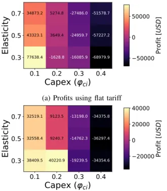
The percentage of public funding for the development of the SAMG modifies the profit of the private investors. Additionally, the implementation of the incentive-based DSMS modifies the profits of the investors compared to the base case. Figure 6 shows the profits of the private investors for the two tariffs, four different percentages of private investment (ϕci) and three different elasticities
of the customers. Figure 6a shows the profits of the private investors using a flat tariff and Figure 6b shows the profits of the private investors using the proposed incentive-based DSMS. The negative values represent that the private investors are loosing money to run the project. Due to this, the figure only considers values of ϕci until 0.4.
The incentive-based DSMS introduces variations in the final price of the energy. Figure 7 shows the daily prices offered to the customers. The continuous line rep-resents the daily average and the shaded area reprep-resents the standard deviation computed over the 365 days of the optimization horizon. The variation in the final price of the energy modify the total payments of the customers. It is interesting to notice in Figure7that the incentive-based DSMS allow to the investors to offer a negative final price for the energy to the customers. A negative final price means that the investor are paying to the customers to consume energy at certain hours of the day. Despite this, the formulation guarantee the reliability of the business model to the investors. Additionally, negative payments can be easily avoided by modifying the limits of the constraint presented in Equation (10).
An interesting analysis as well is how the payments of the customers change when the planner applies the
0.1
0.2
0.3
0.4
Capex (
ci
)
0.3
0.5
0.7
Elasticity
77638.4 -1628.8 -16085.9 -68979.9 43323.1 3649.4 -24959.7 -57227.2 34873.2 5274.8 -27486.0 -51578.750000
0
50000
Profit [
USD
]
(a) Profits using flat tariff
0.1
0.2
0.3
0.4
Capex (
ci
)
0.3
0.5
0.7
Elasticity
38409.5 40220.9 -19239.5 -34354.6 32558.4 9240.7 -14762.3 -36297.4 32519.1 9123.5 -13198.0 -34375.820000
0
20000
40000
Profit [
USD
]
(b) Profits using a DSMS with economic incentives Figure 6: Profit of the private investors for different values of elasticity and different percentages of private investments for the CAPEX.
1 2 3 4 5 6 7 8 9 101112131415161718192021222324
Hour of the day
0.1 0.0 0.1 0.2 0.3
Price [USD]
Flat price
DSMS price
Figure 7: Final prices for the energy offered to the customers.
incentive-based DSMS. The variations in the payments of the customers depend on different aspects. Two of the aspects are the amount of private investment in the project, and the elasticity of the customers. Figure
8 shows a comparison of the customer payments for
the flat and the incentive-based tariffs. Figure 8ashows the total payments of the customers when the planner applies a flat tariff. Figure8bshows the payments of the customers when the planner applies an incentive-based tariff. However, to facilitate the comprehension of the
results, Figure 8b shows the percentage variation of the payments that Eq.28 computes.
%var = PN n=1Γninc− PN n=1Γnf lat PN n=1Γnf lat (28)
0.1
0.2
0.3
0.4
Capex (
ci
)
0.3
0.5
0.7
Elasticity
271101.2 247145.9 260654.0 247145.9 250991.3 254009.3 257899.2 254009.3 255943.6 255399.8 254510.2 255399.8250000
255000
260000
265000
270000
Profit [
USD
]
(a) Payments of the customers using flat tariff (base-line case)
0.1
0.2
0.3
0.4
Capex (
ci
)
0.3
0.5
0.7
Elasticity
-26.54 -13.04 -17.21 -5.57 -7.03 -8.19 -9.51 -8.22 -8.7 -8.66 -8.08 -8.63200000
210000
220000
230000
Profit [
USD
]
(b) Percentage change in payments of the customers using a DSMS with economic incentives
Figure 8: Payments of the customers before and after of the introduction of the DSMS.
By using the results of Figure 8b is possible to
compute the average reduction in the payments of the customers. The average reduction of the payments after the introduction of the DSMS is 10.8%
4.2. Sizing and energy dispatch analysis
The variation in the price shown in Figure 7 incen-tivizes the customers to modify their patterns of con-sumption. Figure 9 shows the variations in the demand after the application of the DSMS for an elasticity of −0.3. To make a clear visualization of the results, only the daily average and the daily standard deviation are shown in the figure. The blue and red continuous lines represent the daily average. The blue and red shaded area represent the standard deviation. The average and the standard deviation are computed over the 8760 hours of simulation.
The proposed methodology uses the tariffs of energy as a DSMS. The tariffs modify the patterns of con-sumption of the customers, which in the end, modify
1 2 3 4 5 6 7 8 9 101112131415161718192021222324
Hour of the day
50 100 150 200 250 300 350
Electrical demand [kW]
Flat demand
DSMS demand
Figure 9: Comparison of the electrical demand before and after the application of the DSMS.
the installed capacities of the energy sources. However, tariffs have superior and inferior limits. The limits in the tariffs and the elasticity of the customers limit the response of the demand. In this regard, the BESS acquires relative importance in the energy dispatch of the SAMG. The BESS can store energy in periods where it is cheaper to generate electricity. The stored energy can supply the demand of the customers when it is more expensive to generate electric energy. This behavior allows the reduction of the installed capacity of the DG when the planner chooses to apply the DSMS. Figure 10 shows the daily average dispatch of the EMS with and without the application of the incentive-based DSMS.
1 2 3 4 5 6 7 8 9 101112131415161718192021222324 Hour of the day
0 50 100 150 200 250 300 350 Energy dispatched [kWh] Right axis DG flat PV flat DG DSMSPV DSMS 0 200 400 600 800 1000 1200
BESS Residual Energy [kWh]
Left axis BESS flat BESS DSMS
Figure 10: Daily average dispatch before and after the application of the DSMS.
4.3. Solar radiation sensitive analysis
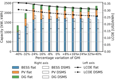
Figure 11 shows the impacts of varying the GHI on facility size and LCOE. Figure 11 reveals the correla-tion between the GHI and the LCOE. When the GHI
increases, the LCOE decreases. This inverse relationship is valid even when the installed photovoltaic capacity remains almost constant. Besides, Figure11 reveals that for reductions in GHI higher than 24%, the fixed sizes of all power sources decrease considerably. Despite this, the LCOE continues to increase.
-40% -32% -24% -16% -8% 0% +8%+16%+24%+32%+40% Percentage variation of GHI
0 500 1000 1500 2000 2500 Capacity [kW, kWh] Right axis BESS flat PV flat DG flat BESS DSMS PV DSMS DG DSMS 0.00 0.05 0.10 0.15 0.20 0.25 0.30 0.35 LCOE [USD/kWh] Left axis LCOE flat LCOE DSMS Figure 11: Comparison of the variations of the size of the energy sources before and after of the application of the DSMS when percentage variation in the GHIs are considered.
4.4. Diesel’ price sensitive analysis
Figure12shows the variations in the sizing of the en-ergy sources when different diesel prices are considered. On the one hand, the flexibility of the DSMS allows the size of the energy sources to be kept almost constant, even when the price of diesel increases 40%. This fact highlights the relevance of the DSMS to face variations in the price of diesel without having to increase the capacities of energy sources. On the other hand, the reduction in the price of diesel allows reducing the in-stalled capacities of PV and BESS. This occurs because the sizing methodology chooses to increase the installed capacities of the DG. By increasing DG capacity, it is possible to supply more demand with diesel generation, taking advantage of low fuel prices.
4.5. BESS costs sensitive analysis
Figure 13 shows the impact of the BESS price on
the sizing of the energy sources of the SAMG. Figure 13 shows that the installed capacities of the BESS de-crease as the purchase price inde-creases. The LCOE main-tains a direct relationship with the acquisition price of BESS. Even when the BESS installed capacity decreases, the LCOE keeps to increase. Furthermore, the sizing
-40% -32% -24% -16% -8% 0% +8%+16%+24%+32%+40% Percentage variation in the price per liter of diesel 0 500 1000 1500 2000 2500 Capacity [kW, kWh] Right axis BESS flat PV flat DG flat BESS DSMS PV DSMS DG DSMS 0.00 0.05 0.10 0.15 0.20 0.25 0.30 0.35 LCOE [USD/kWh] Left axis LCOE flat LCOE DSMS Figure 12: Comparison of the variations of the size of the energy sources before and after of the application of the DSMS when variations in the diesel price are considered.
methodology chooses to increase the DG’s installed capacity when the acquisition price of BESS increases.
Another aspect worth mentioning is that the reduction in LCOE due to the introduction of DSMS remains almost constant. The average reduction in the LCOE when the GHI varies is 15.18%. The average reduction in the LCOE when the price of diesel varies is 15.45%. The average reduction in the LCOE when the BESS price varies is 15.07%. These results highlight the fact that the DSMS can keep the reduction in the LCOE stable despite the variations in GHI, the price of diesel per liter, and the acquisition price of BESS.
-40% -32% -24% -16% -8% 0% +8%+16%+24%+32%+40% Percentage variation in the price per kWh of the BESS 0 500 1000 1500 2000 2500 Capacity [kW, kWh] Right axis BESS flat PV flat DG flat BESS DSMS PV DSMS DG DSMS 0.00 0.05 0.10 0.15 0.20 0.25 0.30 0.35 LCOE [USD/kWh] Left axis LCOE flat LCOE DSMS Figure 13: Comparison of the variations of the size of the energy sources before and after of the application of the DSMS when variations in the BESS price are considered.
5. Conclusions
The present study shows the design of a Demand Side Management Strategy (DSMS) using a Disciplined Convex approach for the planning of islanded micro-grids. The application of the methodology help SAMG planners to compute the sizing of the facilities consid-ering different sources of energy and apply an optimal energy dispatch strategy for the microgrid. Moreover, the methodology allows the planners to compute the expected expenses and revenues of any SAMG project. Additionally, the methodology allows computing the required amount of subsidies from the government to make financially feasible any SAMG project.
The application of sensitivity analysis in a study case shows a reduction in the total costs of the project and the Levelized Cost of the Energy. The study case shows that the profit of the investors decreases when the elasticity of the customers’ increases. In the same way, the payments of the customers reduce when the elasticity of the customers’ increases. This means that the methodology is able to redistribute the excessive profits of the private investors to the customers. However, clear policies are required for SAMG projects to guarantee that the customers benefit from the application of DSMS.
Acknowledgments
The authors wish to thank the Department of Elec-trical, Electronics, and Telecommunications Engineer-ing (Escuela de Ingenierías Eléctrica, Electrónica y de Telecomunicaciones); the Vice-Rectorate for Research and Extension (Vicerrectoría de Investigación y Ex-tensión) from the Universidad Industrial de Santander (Project 8585); and the Administrative Department of Science, Technology, and Innovation (Departamento Administrativo de Ciencia, Tecnología e Innovación)-COLCIENCIAS (Contract No. 80740-191-2019, Fund-ing source). The authors also wish to thank to the Emerging Leaders for the Americas Program (ELAP), offered by the government of Canada, to the Latino-American and Caribbean community.
REFERENCES
[1] W. S. Ebhota, “Power accessibility, fossil fuel and the exploitation of small hydropower technology in sub-saharan africa,” International Journal of Sustainable Energy Planning and Management, vol. 19, pp. 13–28, 2019. [Online]. Available:
https://doi.org/10.5278/ijsepm.2019.19.3
[2] B. Brahim, “Performance investigation of a hybrid PV-diesel power system for remote areas,” International Journal of Energy Research, vol. 43, no. 2, pp. 1019–1031, 2019. [Online]. Available:https://doi.org/10.1002/er.4301
[3] T. Tu, G. P. Rajarathnam, and A. M. Vassallo, “Optimal sizing and operating strategy of a stand-alone generation–load–storage system: An island case study,” Energy Storage, no. September 2019, pp. 1–22, 2019. [Online]. Available: https://doi.org/10. 1002/est2.102
[4] V. Kumtepeli, Y. Zhao, M. Naumann, A. Tripathi, Y. Wang, A. Jossen, and H. Hesse, “Design and analysis of an aging-aware energy management system for islanded grids using mixed-integer quadratic programming,” International Journal of Energy Research, vol. 43, no. 9, pp. 4127–4147, 2019. [Online]. Available:https://doi.org/10.1002/er.4512
[5] C. Domingueza, K. Orehounig, and J. Carmeliet, “Modelling of rural electrical appliances ownership in developing countries to project their electricity demand: A case study of sub-Saharan Africa,” International Journal of Sustainable Energy Planning and Management, vol. 22, pp. 5–16, 2019. [Online]. Available:
https://doi.org/10.5278/ijsepm.2564
[6] I. O. Ogundari, Y. O. Akinwale, A. O. Adepoju, M. K. Atoyebi, and J. B. Akarakiri, “Suburban housing development and off-grid electric power supply assessment for North-Central Nigeria,” International Journal of Sustainable Energy Planning and Management, vol. 12, pp. 47–64, 2017. [Online]. Available:https://doi.org/10.5278/ijsepm.2017.12.5
[7] Z. Xu, M. Nthontho, and S. Chowdhury, “Rural electrification implementation strategies through microgrid approach in South African context,” International Journal of Electrical Power and Energy Systems, vol. 82, pp. 452–465, 2016. [Online]. Available:https://doi.org/10.1016/j.ijepes.2016.03.037
[8] J. Tariq, “Energy management using storage to facilitate high shares of variable renewable energy,” International Journal of Sustainable Energy Planning and Management, vol. 25, pp. 61–76, 2020. [Online]. Available: https://doi.org/10.5278/ijse pm.3453
[9] H. Meschede, J. Hesselbach, M. Child, and C. Breyer, “On the impact of probabilistic weather data on the economically optimal design of renewable energy systems – A case study of la gomera island,” International Journal of Sustainable Energy Planning and Management, vol. 23, pp. 15–26, 2019. [Online]. Available:https://doi.org/10.5278/ijsepm.3142
[10] J. Aghaei and M. I. Alizadeh, “Demand response in smart electricity grids equipped with renewable energy sources: A review,” Renewable and Sustainable Energy Reviews, vol. 18, pp. 64–72, 2013. [Online]. Available:
http://dx.doi.org/10.1016/j.rser.2012.09.019
[11] N. Cicek and H. Delic, “Demand Response Management for Smart Grids With Wind Power,” Transactions on Sustainable Energy, vol. 6, no. 2, pp. 625–634, 2015. [Online]. Available:
http://dx.doi.org/10.1109/tste.2015.2403134
[12] L. Gelazanskas and K. A. A. Gamage, “Demand side management in smart grid: A review and proposals for future direction,” Sustainable Cities and Society, pp. 1–9, 2013. [Online]. Available:http://dx.doi.org/10.1016/j.scs.2013.11.001
[13] M. H. Albadi and E. F. El-Saadany, “A summary of demand response in electricity markets,” Electric Power Systems Research, vol. 78, no. 11, pp. 1989–1996, 2008. [Online]. Available:https://doi.org/10.1016/j.epsr.2008.04.002
[14] K. Kostková, Omelina, P. Kyˇcina, and P. Jamrich, “An introduction to load management,” Electric Power Systems Research, vol. 95, pp. 184–191, 2013. [Online]. Available:
https://doi.org/10.1016/j.epsr.2012.09.006
[15] M. Franz, Nico Peterschmidt, Michael Rohrer, and Bozhil Kondev, “Mini-grid Policy Toolkit,” Alliance for Rural
Electrification, Eschborn, Tech. Rep., 2014. [Online].
Available: https://www.ruralelec.org/sites/default/files/inensus-t oolkit-en-21x21-web-ok.pdf
[16] T. Reber, S. Booth, D. Cutler, X. Li, J. Salasovich, and W. Ratterman, “Tariff Considerations for Micro-Grids in Sub-Saharan Africa,” NREL, Tech. Rep. February, 2018. [Online]. Available:https://www.nrel.gov/docs/fy18osti/69044.pdf
[17] M. Jin, W. Feng, P. Liu, C. Marnay, and C. Spanos, “MOD-DR: Microgrid optimal dispatch with demand response,” Applied Energy, vol. 187, pp. 758–776, 2017. [Online]. Available:
http://dx.doi.org/10.1016/j.apenergy.2016.11.093
[18] C. E. Casillas and D. M. Kammen, “The delivery of low-cost, low-carbon rural energy services,” Energy Policy, vol. 39, no. 8, pp. 4520–4528, 2011. [Online]. Available:
http://dx.doi.org/10.1016/j.enpol.2011.04.018
[19] R. Palma-Behnke, C. Benavides, E. Aranda, J. Llanos, and D. Sáez, “Energy management system for a renewable based microgrid with a demand side management mechanism,” in Symposium Series on Computational Intelligence - Applications in Smart Grid, Paris, 2011, pp. 131–138. [Online]. Available:
http://dx.doi.org/10.1109/CIASG.2011.5953338
[20] M. Mazidi, A. Zakariazadeh, S. Jadid, and P. Siano, “Integrated scheduling of renewable generation and demand response programs in a microgrid,” Energy Conversion and Management, vol. 86, pp. 1118–1127, 2014. [Online]. Available:http://dx.doi.org/10.1016/j.enconman.2014.06.078
[21] G. R. Aghajani, H. A. Shayanfar, and H. Shayeghi,
“Demand side management in a smart micro-grid in the presence of renewable generation and demand response,” Energy, vol. 126, pp. 622–637, 2017. [Online]. Available:
http://dx.doi.org/10.1016/j.energy.2017.03.051
[22] C. Wu, H. Mohsenian-Rad, J. Huang, and A. Y. Wang, “Demand side management for Wind Power Integration in microgrid using dynamic potential game theory,” in GLOBECOM Workshops, 2011, pp. 1199–1204. [Online]. Available: http: //dx.doi.org/10.1109/GLOCOMW.2011.6162371
[23] F. Weston, “Integrated Resource Planning:
His-tory and Principles,” in 27th National
Reg-ulatory Conference, 2009. [Online].
Avail-able: https://www.raponline.org/wp-content/uploads/2016/05/ra p-weston-integratedresourceplanningoverview-2009-05-20.pdf
[24] International Rivers, “An Introduction to
Inte-grated Resource Planning,” 2013. [Online].
Avail-able: https://www.internationalrivers.org/resources/an-introduct ion-to-integrated-resources-planning-8143
[25] Lan Zhu, Zheng Yan, Wei-Jen Lee, Xiu Yang, and Yang Fu, “Direct load control in microgrid to enhance the performance of integrated resources planning,” in Industrial & Commercial Power Systems Technical Conference, 2014, pp. 1–7. [Online]. Available:https://doi.org/10.1109/TIA.2015.2413960
[26] L. Zhu, X. Zhou, X.-P. Zhang, Z. Yan, S. Guo, and L. Tang, “Integrated resources planning in microgrids considering interruptible loads and shiftable loads,” Journal of Modern Power Systems and Clean Energy, vol. 6, no. 4, pp. 802–815, 2018. [Online]. Available: https://doi.org/10.1007/s40565-017-0357-1
[27] S. Kahrobaee, S. Asgarpoor, and W. Qiao, “Optimum sizing of distributed generation and storage capacity in
smart households,” IEEE Transactions on Smart Grid,
vol. 4, no. 4, pp. 1791–1801, 2013. [Online]. Available:
http://dx.doi.org/10.1109/TSG.2013.2278783
[28] O. Erdinc, N. G. Paterakis, I. N. Pappi, A. G. Bakirtzis, and J. P. Catalão, “A new perspective for sizing of distributed generation and energy storage for smart households under demand response,” Applied Energy, vol. 143, pp. 26–37, 2015. [Online]. Available:http://dx.doi.org/10.1016/j.apenergy.2015.01.025
[29] S. Nojavan, M. Majidi, and N. N. Esfetanaj, “An efficient cost-reliability optimization model for optimal siting and sizing of energy storage system in a microgrid in the presence
of responsible load management,” Energy, vol. 139, pp. 89–97, 2017. [Online]. Available:https://doi.org/10.1016/j.ener gy.2017.07.148
[30] M. Majidi, S. Nojavan, and K. Zare, “Optimal Sizing of Energy Storage System in a Renewable-Based Microgrid Under Flexible Demand Side Management Considering Reliability and Uncertainties,” Journal of Operation and Automation in Power Engineering, vol. 5, no. 2, pp. 205–214, 2017. [Online]. Available:http://dx.doi.org/10.22098/joape.2017.3356.1268
[31] V. Mehra, R. Amatya, and R. J. Ram, “Estimating the value of demand-side management in low-cost, solar micro-grids,” Energy, vol. 163, pp. 74–87, 2018. [Online]. Available:
https://doi.org/10.1016/j.energy.2018.07.204
[32] V. Mehra, “Optimal Sizing of Solar and Battery Assets in Decentralized Micro-Grids with Demand-Side Management,” Ph.D. dissertation, Massachusetts Institute of Technology, 2017. [Online]. Available: https://dspace.mit.edu/handle/1721. 1/108959
[33] J. Kumar, B. V. Suryakiran, A. Verma, and T. S. Bhatti, “Analysis of techno-economic viability with demand response strategy of a grid-connected microgrid model for enhanced rural electrification in Uttar Pradesh state, India,” Energy,
vol. 178, pp. 176–185, 2019. [Online]. Available: https:
//doi.org/10.1016/j.energy.2019.04.105
[34] G. Notton, V. Lazarov, Z. Zarkov, and L. Stoyanov,
“Optimization of hybrid systems with renewable energy sources : Trends for research,” 2006 1st International Symposium on Environment Identities and Mediterranean Area, ISEIM, pp. 144–149, 2006. [Online]. Available: http: //dx.doi.org/10.1109/ISEIMA.2006.344942
[35] J. L. Bernal-Agustín and R. Dufo-López, “Simulation and optimization of stand-alone hybrid renewable energy systems,” Renewable and Sustainable Energy Reviews, vol. 13, no. 8, pp. 2111–2118, 2009. [Online]. Available:https://doi.org/10.1016/ j.rser.2009.01.010
[36] P. Samadi, A.-H. Mohsenian-Rad, R. Schober, V. W.S., Wong, and J. Jatskevich, “Optimal Real-time Pricing Algorithm Based on Utility Maximization for Smart Grid,” in International Conference on Smart Grid Communications, no. June 13, 2010, pp. 415–420. [Online]. Available: http://dx.doi.org/10. 1109/SMARTGRID.2010.5622077
[37] R. Yu, W. Yang, and S. Rahardja, “A Statistical Demand-Price Model With Its Application in Optimal Real-Time Price,” Transactions on Smart Grid, pp. 1–9, 2012. [Online]. Available:
http://dx.doi.org/10.1109/TSG.2012.2217400
[38] H. Aalami, G. R. Yousefi, and M. Parsa Moghadam, “Demand response model considering EDRP and TOU programs,”
Transmission and Distribution Exposition Conference:
Powering Toward the Future, 2008. [Online]. Available:
http://dx.doi.org/10.1109/TDC.2008.4517059
[39] A. Gillespie, Foundations of Economics. Oxford University
Press, 2007. [Online]. Available: https://books.google.ca/book s?id=9NoT4gnYvPMC
[40] Ausgrid, “Appendix 5: Australian Price Elasticity of Demand,” Ausgrid, Tech. Rep. November, 2015. [Online]. Available:
https://bit.ly/2OfmeR2
[41] “Centro nacional de monitoreo, informe mensual de telemetría,”
http://190.216.196.84/cnm/info_mes.php, accessed:
2019-12-09.
[42] A. Chauhan and R. P. Saini, “A review on Integrated Renewable Energy System based power generation for stand-alone applications: Configurations, storage options, sizing methodologies and control,” Renewable and Sustainable
Energy Reviews, vol. 38, pp. 99–120, 2014. [Online].
Available:http://dx.doi.org/10.1016/j.rser.2014.05.079
[43] S. Diaf, G. Notton, M. Belhamel, M. Haddadi, and A. Louche,
“Design and techno-economical optimization for hybrid
PV/wind system under various meteorological conditions,” Applied Energy, vol. 85, no. 10, pp. 968–987, 2008. [Online]. Available:https://doi.org/10.1016/j.apenergy.2008.02.012
[44] B. Li, R. Roche, D. Paire, and A. Miraoui, “Sizing of a stand-alone microgrid considering electric power, cooling/heating, hydrogen loads and hydrogen storage degradation,” Applied Energy, vol. 205, no. July, pp. 1244–1259, 2017. [Online]. Available:https://doi.org/10.1016/j.apenergy.2017.08.142
[45] J. Zhang, K. J. Li, M. Wang, W. J. Lee, H. Gao, C. Zhang, and K. Li, “A Bi-Level Program for the Planning of an Islanded Microgrid Including CAES,” IEEE Transactions on Industry Applications, vol. 52, no. 4, pp. 2768–2777, 2016. [Online]. Available:http://dx.doi.org/10.1109/TIA.2016.2539246
[46] F. Lasnier, Photovoltaic Engineering Handbook. Taylor & Francis, 1990. [Online]. Available: https://books.google.ca/bo oks?id=1ZuVGsySttQC
[47] E. Skoplaki and J. A. Palyvos, “Operating temperature of photovoltaic modules: A survey of pertinent correlations,” Renewable Energy, vol. 34, no. 1, pp. 23–29, 2009. [Online]. Available:https://doi.org/10.1016/j.renene.2008.04.009
[48] J. A. Duffie and W. A. Beckman, Solar Engineering of Thermal Processes, 4th ed. Wiley, 2013. [Online]. Available:http://eu.w iley.com/WileyCDA/WileyTitle/productCd-0470873663.html
[49] T. Markvart, Ed., Solar electricity, 2nd ed. Wiley, 2000.
[Online]. Available: https://www.wiley.com/en-us/Solar+Electr icity,+2nd+Edition-p-9780471988526
[50] X. Zhang, Y. Wang, J. Wu, and Z. Chen, “A novel method for lithium-ion battery state of energy and state of power estimation based on multi-time-scale filter,” Applied Energy, vol. 216, no. February, pp. 442–451, 2018. [Online]. Available:
https://doi.org/10.1016/j.apenergy.2018.02.117
[51] P. Arun, R. Banerjee, and S. Bandyopadhyay, “Optimum sizing of battery-integrated diesel generator for remote electrification through design-space approach,” Energy, vol. 33,
no. 7, pp. 1155–1168, 2008. [Online]. Available: https:
//doi.org/10.1016/j.energy.2008.02.008
[52] S. Ashok, “Optimised model for community-based hybrid energy system,” Renewable Energy, vol. 32, pp. 1155– 1164, 2006. [Online]. Available:https://doi.org/10.1016/j.rene ne.2006.04.008
[53] M. S. Scioletti, A. M. Newman, J. K. Goodman, A. J. Zolan, and S. Leyffer, “Optimal design and dispatch of a system of diesel generators, photovoltaics and batteries for remote locations,” Optimization and Engineering, vol. 18,
no. 3, pp. 755–792, 2017. [Online]. Available: https: