HAL Id: hal-03025174
https://hal.archives-ouvertes.fr/hal-03025174
Submitted on 7 Dec 2020
HAL is a multi-disciplinary open access
archive for the deposit and dissemination of
sci-entific research documents, whether they are
pub-lished or not. The documents may come from
L’archive ouverte pluridisciplinaire HAL, est
destinée au dépôt et à la diffusion de documents
scientifiques de niveau recherche, publiés ou non,
émanant des établissements d’enseignement et de
Seismological evidence for thermo-chemical
heterogeneity in Earth’s continental mantle
Federico Munch, Amir Khan, Benoit Tauzin, Martin van Driel, Domenico
Giardini
To cite this version:
Federico Munch, Amir Khan, Benoit Tauzin, Martin van Driel, Domenico Giardini. Seismological
ev-idence for thermo-chemical heterogeneity in Earth’s continental mantle. Earth and Planetary Science
Letters, Elsevier, 2020, 539, pp.116240. �10.1016/j.epsl.2020.116240�. �hal-03025174�
Seismological evidence for thermo-chemical
heterogeneity in Earth’s continental mantle
Federico D. Munch1,∗, Amir Khan2,1, Benoit Tauzin3,4, Martin van Driel1,
Domenico Giardini1
Abstract
Earth’s thermo-chemical structure exerts a fundamental control on mantle con-vection, plate tectonics, and surface volcanism. There are indications that man-tle convection occurs as an intermittent-stage process between layered and whole mantle convection in interaction with a compositional stratification at 660 km depth. However, the presence and possible role of any compositional layering in the mantle remains to be ascertained and understood. By interfacing inversion of a novel global seismic data set with petrologic phase equilibrium calcula-tions, we show that a compositional boundary is not required to explain short-and long-period seismic data sensitive to the upper mantle short-and transition zone beneath stable continental regions; yet, radial enrichment in basaltic material reproduces part of the complexity present in the data recorded near subduction zones and volcanically active regions. Our findings further indicate that: 1) cratonic regions are characterized by low mantle potential temperatures and sig-nificant lateral variability in mantle composition; and 2) chemical equilibration seems more difficult to achieve beneath stable cratonic regions. These findings suggest that the lithologic integrity of the subducted basalt and harzburgite
∗Corresponding author
Email address: fmunch@seismo.berkeley.edu (Federico D. Munch)
1Institute of Geophysics, ETH Zurich, Switzerland.
Present address: Berkeley Seismological Laboratory, University of California, Berkeley, CA 94720, USA.
2Institute of Theoretical Physics, University of Zurich, Switzerland.
3Laboratoire de G´eologie de Lyon, Terre, Plan`etes, Environnement, Universit´e de Lyon,
Ecole Normale Sup´erieure de Lyon, CNRS, France.
4Research School of Earth Sciences, Australian National University, Australia.
*Manuscript (tex)
may be better preserved for geologically significant times underneath cratonic regions.
Keywords: Mantle thermo-chemistry, receiver functions, surface wave
dispersion, petrologic phase equilibrium calculations
1. Introduction
1
Since the recognition that plate tectonics is driven by solid-state mantle
2
convection in the late 1960s, geoscientists have been debating mantle
thermo-3
chemical structure and the detailed morphology of convection. Geochemical
4
analysis of volcanic rocks (e.g., Pearson et al., 2003) support the existence of
5
distinct reservoirs suggesting the mantle to be compositionally and
dynami-6
cally layered, with the 660–km seismic discontinuity acting as compositional
7
boundary. However, three-dimensional images of mantle structure from seismic
8
tomography (e.g., French and Romanowicz, 2014; Schaeffer and Lebedev, 2013)
9
indicate that subducted oceanic plates (known as slabs) can penetrate into the
10
lower mantle as well as stagnate in the mantle transition zone (MTZ; region
11
between 410 and 660 km depth) and around ∼1000 km depth, which rules out
12
global layering at 660–km and appears to support whole-mantle convection
in-13
stead. A range of hypotheses have been proposed to reconcile these observations
14
(e.g., leaky layering at 660 km, layering deeper in the mantle, and ubiquitous
15
compositional heterogeneity), yet the detailed morphology of convection
pat-16
terns remains a matter of debate. The key question is whether the 660–km
17
discontinuity is caused by a change in chemical composition (e.g., Anderson,
18
2007) in addition to the endothermic ringwoodite→bridgmanite+ferropericlase
19
phase transition (e.g., Ita and Stixrude, 1992).
20
Numerical modeling of subduction suggests that a lower-mantle enrichment
21
in basalt (∼8% with respect to the upper mantle) can explain slab stagnation
22
at 660 and 1000 km depth, in the presence of whole-mantle convection (e.g.,
23
Ballmer et al., 2015). This finding suggests that mantle convection occurs in an
24
intermittent mode between layered- and whole-mantle convection, where slabs
penetrate intermittently in space and time, while a globally-averaged
composi-26
tional stratification at 660 km depth is maintained (e.g., Tackley, 2000).
Sup-27
porting evidence arises from direct comparison of one-dimensional Earth
ref-28
erence velocity models and seismic observations sensitive to the bulk velocity
29
structure of the mantle (P- and S-wave travel times and surface wave data)
30
with estimates for a pyrolitic (Ringwood, 1975) and adabatic mantle based on
31
insights obtained from theoretical and experimental mineral physics. These
32
studies report that pyrolitic and adiabatic mantle models cannot explain global
33
observations (e.g., Cobden et al., 2008) and suggest that the lower mantle is
ei-34
ther enriched (e.g., Murakami et al., 2012) or depleted (e.g., Khan et al., 2008)
35
in silicon relative to the upper mantle. However, detailed analysis of SS and PP
36
precursors that are sensitive to MTZ discontinuities, indicate that the observed
37
amplitude variations (and even the absence of PP precursors in certain regions)
38
are well-explained by lateral changes in mantle temperature or aluminium
con-39
tent for a pyrolite mantle (Deuss et al., 2006).
40
Here, we investigate whether compositional mantle stratification is required
41
to jointly explain seismic data sensitive to upper mantle and transition zone
42
beneath a number of different tectonic settings by implementing a methodology
43
that interfaces geophysical inversion of seismic data with self-consistent
calcu-44
lations of mineral phase equilibria (Munch et al., 2018). The prediction of rock
45
mineralogy and its elastic properties as a function of pressure, temperature, and
46
bulk composition allows for self-consistent determination of depth and sharpness
47
of the 410– and 660–km seismic discontinuities as well as upper mantle
veloc-48
ities. This enables the joint analysis of P-to-s receiver functions and Rayleigh
49
surface wave dispersion data to directly infer global lateral variations of
man-50
tle temperature and composition. Until now, both data types have never been
51
combined to resolve the structure down to the base of the MTZ.
2. Materials and Methods
53
2.1. P-to-s receiver functions
54
P-to-s receiver functions (hereinafter RF) are the records of compressional
55
waves that convert into shear waves when encountering a discontinuity in
mate-56
rial properties and are sensitive to sharp seismic discontinuities within a
depth-57
dependent annulus underneath seismic stations (see Figure 1). Conversions
58
occurring at the 410–km (P410s) and 660–km (P660s) discontinuities are
rou-59
tinely used for detection of mineralogical phase changes at 410 and 660 km
60
depth (e.g., Helffrich, 2000; Lawrence and Shearer, 2006b; Tauzin et al., 2008),
61
but are rarely inverted to determine MTZ elastic structure (e.g., Schmandt,
62
2012; Lawrence and Shearer, 2006a). Building on previous experience (Munch
63
et al., 2018), we here invert RF waveforms to directly map global variations in
64
mantle temperature and composition.
65
To this end, we first constructed a new global high-quality dataset of RF
66
waveforms. The data consists of three-component seismograms recorded at 155
67
broad-band permanent stations between 1997 and 2018. In order to ensure a
68
good signal-to-noise ratio, only teleseismic events for epicentral distances
be-69
tween 40◦and 95◦ with magnitudes larger than 6 were selected. RF waveforms
70
at each station were obtained by: 1) filtering of the records in the period range
71
1–100 s; 2) rotation of the seismograms into radial, transverse, and vertical
72
components; 3) calculation of signal-to-noise ratio between the maximum
ampli-73
tude of the signal and the averaged root-mean-square of the vertical component;
74
4) construction of RF waveforms through iterative time domain deconvolution
75
(Ligorria and Ammon, 1999) for traces with signal-to-noise ratio larger than
76
5; and 5) low-pass filtering of the RF waveforms to remove frequencies higher
77
than 0.2 Hz. Finally, RF waveforms were corrected for move-out (using IASP91
78
velocity model and a reference slowness of 6.5 s/deg) and subsequently stacked.
79
Error on the stacked amplitudes were estimated using a bootstrap resampling
80
approach (Efron and Tibshirani, 1991).
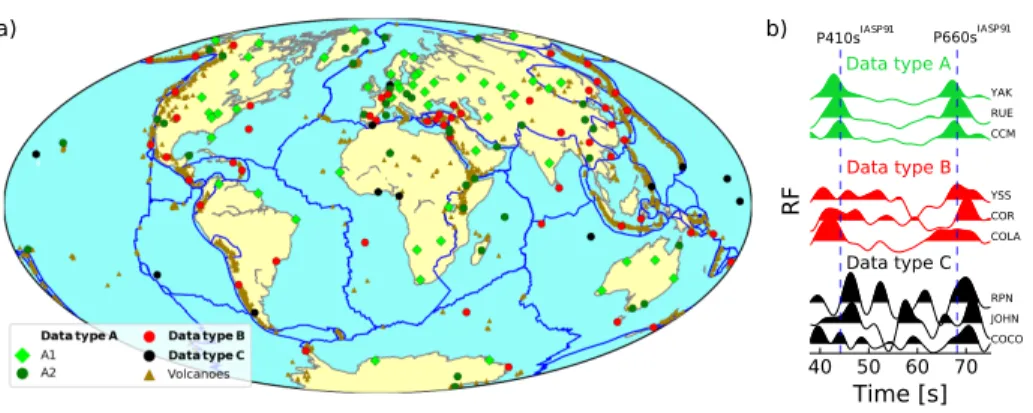
2.2. Data selection
82
The inversion of RFs requires careful waveform inspection to ensure high
83
quality data. The stations were classified into three quality classes by visual
84
inspection of the stacked RF waveforms (see Figure 2 and Table S1). Type-A
85
stations correspond to RF waveforms with high signal-to-noise ratio and clear
86
P410s and P660s signals. Type-B stations are characterized by RF waveforms
87
with high signal-to-noise ratio but the signals corresponding to either the P410s
88
or P660s conversions cannot be clearly isolated due to the potential presence
89
of interfering seismic phases or complex three-dimensional structure. Type-C
90
stations correspond to locations where only a small number of data could be
91
stacked resulting in highly noisy RF waveforms with no clear P410s and P660s
92
signals.
93
We found 48 stations for which the signals corresponding to either the P410s
94
or P660s conversions cannot be unambiguously isolated (Type–B stations in
95
Figure 2 and Figure S1). These stations are often located in regions where
96
structure has previously been identified in seismic tomography models (e.g.,
97
Schaeffer and Lebedev, 2013) such as subducted slabs in northeast Asia and the
98
Mediterranean Sea. Our analysis focuses on 103 stations (Type–A stations in
99
Figure 2) mainly located away from plate boundaries, where the RF waveforms
100
can be accurately modeled with relatively low computational cost by methods
101
that simulate full seismic wave propagation from source to receiver in spherical
102
1D Earth models.
103
2.3. Rayleigh wave dispersion data
104
Rayleigh wave phase velocities are sensitive to the bulk velocity structure
105
of the upper mantle and provide a better global coverage than the RFs, but
106
with lower lateral resolution (∼650 km). Here, we enhanced our RF data by
107
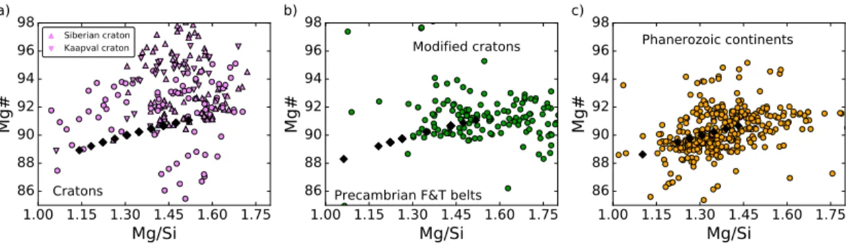
extracting phase velocity dispersion curves for each station from the most recent
108
available global data set of Rayleigh wave phase velocity dispersion (Durand
109
et al., 2015). The data set consists of 60 phase velocity maps and uncertainties
0 400 800 200 600 1000 P660s P410s P Transition zone 410-km 660-km
Figure 1: Schematic representation of teleseismic P–to–s waves scattered in the mantle tran-sition zone and recorded at a seismic station (black triangle) located at an epicentral distance of 40◦. Solid and dashed lines correspond to P and S ray path segments, respectively. The distance from the receiver along the 410–km and 660–km discontinuities is indicated in kilo-meters. The conversion points at 410–km and 660–km depth are laterally shifted from the station by ∼150 km and ∼250 km, respectively. Figure modified from Tauzin et al. (2008).
8 a) 40 50 60 70 Time [s] RF COCO JOHN RPN COLA COR YSS CCM RUE YAK Data type A Data type B Data type C P410sIASP91 P660sIASP91 b)
Figure 2: Geographic distribution of seismic stations. a) In all 155 seismic stations were considered and classified by data quality (type A, B, and C). Type A stations are subdivided into two further categories based on the data fit, labelled “A1” and “A2”. b) Examples of observed receiver functions (RF) for each data class.
covering the period range 40–250 s for the fundamental mode and up to the
111
fifth overtone on a 2◦× 2◦ grid.
112
We would like to note that this data set is the result of a global tomographic
113
inversion and hence is affected by the chosen regularization. If overly damped,
114
phase velocity maps will be smoothened as a result of which dispersion curves
115
and RF waveforms might possibly sense slightly different structure.
116
2.4. Model parameterization and forward problem
117
The crustal structure underneath each station is described in terms of a
118
set of layers with variable S–wave velocity Vi
s and thickness di (i = 1, ..., 5).
119
Mantle velocities below the Moho are derived from a set of model parameters
120
that describe mantle composition and thermal structure (Munch et al., 2018).
121
The former is parameterized in terms of a single variable (f) that represents
122
the amount of basalt in a basalt-harzburgite mixture, with the composition of
123
basalt and harzburgite end-members described using the CFMASNa chemical
124
model system comprising the oxides CaO-MgO-FeO-Al2O3-SiO2-Na2O. Mantle
125
thermal structure is delineated by a conductive lithosphere (linear gradient) on
126
top of an adiabatic geotherm. The lithospheric temperature is defined by the
temperature (T0) at the surface and the temperature (Tlit) at the bottom of 128
the lithosphere. The bottom of the lithosphere (zlit) corresponds to the depth
129
at which the conductive lithospheric geotherm intersects the mantle adiabat
130
defined by the entropy of the lithology at the temperature Tlitand pressure Plit.
131
This simplification allow us to treat continents as conducting lids that float atop
132
the convecting mantle. The pressure profile is obtained by integrating the load
133
from the surface.
134
Mantle mineralogy and its elastic properties as a function of depth are
com-135
puted by means of free-energy minimization (Connolly, 2009; Stixrude and
136
Lithgow-Bertelloni, 2011). Furthermore, shear attenuation is self-consistently
137
derived from the shear modulus, temperature, and pressure profiles using the
138
extended Burgers viscoelastic model (e.g., Bagheri et al., 2019). The resulting
139
velocity and attenuation profiles are then used to compute synthetic RF
wave-140
forms and Rayleigh wave phase velocities. The former are computed with the
141
reflectivity method (Muller, 1985) replicating the slowness distribution recorded
142
at each station and the same processing scheme applied on the observed
seismo-143
grams. The latter are estimated using a spectral element-based python toolbox
144
(Kemper et al., 2020; A spectral element normal mode code for the generation
145
of synthetic seismograms; manuscript in preparation).
146
The choice of chemical model parameterization relies on its proximity to
147
mantle dynamical processes, i.e., partial melting of mantle material along
mid-148
ocean ridges. This process produces a basaltic crust and its depleted residue
149
(harzburgite), which are cycled back into the mantle at subduction zones and
150
become entrained in the mantle flow and remixed. In spite of its simplicity, the
151
concept of distinct chemical end-member compositions has been found to
pro-152
vide an adequate description of mantle chemistry, at least from a geophysical
153
point of view (e.g., Xu et al., 2008; Khan et al., 2009; Ritsema et al., 2009).
154
Furthermore, the use of the CFMASNa model chemical system allows us to
155
account for the effect of transitions in the olivine, garnet, and pyroxene
compo-156
nents of the mantle. As a consequence, and in contrast to usual seismological
157
practice (e.g., Lawrence and Shearer, 2006b; Tauzin et al., 2008; Schmandt,
2012; Cottaar and Deuss, 2016), estimates of MTZ topography, volumetric
ve-159
locities, and temperature derived here are independent of tomographic models
160
or assumptions about the Clapeyron slope of pure (Mg,Fe)2SiO4-phases.
161
The thermodynamic model presented here precludes consideration of redox
162
effects (e.g., Cline II et al., 2018) as well as minor phases and components such
163
as H2O and melt due to lack of thermodynamic data. With regard to potential
164
errors introduced by neglecting the effect of water, experimental evidence
sug-165
gests that the presence of water would tend to thicken the transition zone by
166
moving the olivine-wadsleyite transition up, while deepening the dissociation of
167
ringwoodite (Frost and Dolejˇs, 2007; Ghosh et al., 2013). However, as discussed
168
by Thio et al. (2015), it is currently not possible to quantify the effect of
wa-169
ter on phase transitions because of the large uncertainties in thermodynamic
170
data. In addition, the analyses performed by Thio et al. (2015) and Wang et al.
171
(2018), where it is suggested that hydration of ringwoodite can significantly
172
reduce elastic wave velocities, are based on experiments performed at ambient
173
pressure conditions. A recent study by Schulze et al. (2018) showed that the
174
hydration-induced reduction of seismic velocities almost vanishes at the
tem-175
perature and pressure conditions of the transition zone. Density and elastic
176
moduli are estimated to be accurate to within ∼0.5% and ∼1–2%, respectively
177
(Connolly and Khan, 2016).
178
2.5. Inverse problem
179
The inverse problem is solved within a Bayesian framework where the
so-180
lution is described in terms of the posterior probability distribution σ(m|d) ∝
181
ρ(m)L(m|d). The probability distribution ρ(m) describes the a priori
informa-182
tion on model parameters (summarized in Table S2) and the likelihood function
183
L(m|d) represents a measure of the similarity between the observed data d and
184
the predictions from model m = (Tlit, zlit, f, V1s, . . . , V5s, d1, . . . , d5). As time
185
windows containing considerably small or no signal can introduce undesirable
186
noise into the misfit function and unnecessarily increase the complexity of the
187
misfit surface (Munch et al., 2018), the modeled and observed RF waveforms
are compared in three time windows defined by visual inspection of the
ob-189
served waveforms to include: 1) crustal signals (−5 s < t < 30 s); 2) the P410s
190
conversion (generally observed in the time window 40 s–50 s); and 3) the P660s
191
conversion (typically recorded within the time window 60 s–80 s). Consequently,
192
the likelihood function can be written as
193 L(m|d) ∝ exp ( −1 2 3 X i=1 φRFi (m|d) −1 2 5 X i=0 φSWi (m|d) ) , (1) with 194 φRFi (m|d) = 1 3Ni Ni X j=1 " RFobserved(tj) − RFmodeled(m, tj) δRFobserved(tj) #2 (2) and 195 φSWi (m|d) = 1 6Mi Mi X j=1 " Ci,observedp (Tj) − Ci,modeledp (Tj, m) δCi,observedp (Tj) #2 , (3) where Ci
p(Tj) denotes Rayleigh wave phase velocities for mode i and period
196
Tj with Mi being the number of observed periods for each mode, δ observed
197
uncertainties for each data type, and Ni the number of samples in each time
198
window of interest.
199
We sample the posterior distribution in the model space by combining a
200
Metropolis-Hastings Markov chain Monte Carlo (McMC) method (e.g., Mosegaard
201
and Tarantola, 1995) with a stochastic optimization technique (Hansen et al.,
202
2011). The latter is used to obtain a good initial model for the McMC
algo-203
rithm. This strategy improves the efficiency of the McMC method by
signif-204
icantly reducing the burn-in period. The McMC sampling is performed using
205
10 independent chains (with a total length of 10,000 iterations) characterized
206
by identical initial models but different randomly chosen initial perturbations.
207
This strategy allows for sampling 100,000 models with moderate computational
208
cost (∼3 days using 10 cores). Finally, the 50,000 best-fitting candidates are
209
used to build histograms of the marginal probability distribution of each model
210
parameter.
3. Results
212
The seismic data are inverted using a Bayesian framework to provide
es-213
timates of model range and uncertainty (see Sections 2.4 and 2.5). At each
214
station, we recover marginal probability distributions of parameters describing
215
crustal and mantle thermo-chemical structure (Figure 3b). By-products are
as-216
sociated elastic profiles (Vp, Vs, and density) for the upper mantle down to
217
1000 km depth (Figure 3b). The sampled models must predict the observed
218
Rayleigh wave phase velocities for the fundamental mode and overtones, as well
219
as the main features of the observed RF waveforms (Figure 3a). Type-A
sta-220
tions are further separated into two categories based on the quality of the data
221
fit (Figure 2a) determined by visual inspection of the RF waveforms (Figure 3c
222
and Figure S1) and Rayleigh wave dispersion curves (Figures S2–S3).
223
Our results suggest significant regional deviations from a compositionally
224
uniform and adiabatic mantle. The retrieved models succeed in explaining the
225
observed data in the inner part of continents (A1 stations in Figure 2a), but not
226
near active plate boundaries such as in the western US or northeast Eurasia,
227
in oceanic regions (Hawaii, Iceland, Samoa), or regions of intra-plate
volcan-228
ism such as the Afar (A2 stations in Figure 2a). Among 93 stations in the
229
continents, we succeed to fit the seismic data at 53 stations: 11 stations in
230
Phanerozoic provinces of age younger than 600 Myr, 20 stations in 600-2000
231
Myr old precambrian platforms, and 22 stations in cratonic regions older than
232
2.2 Byr (Figure 4a).
233
We find mantle potential temperatures – equivalent to the temperature that
234
the mantle would have at the surface, if it ascended along an adiabat
with-235
out undergoing melting (McKenzie and Bickle, 1988) – ranging between 1450–
236
1700 K (Figure 4b). These estimates are in good agreement with experimentally
237
determined mantle potential temperatures (1610±35 K) based on a pyrolitic
238
composition (Katsura et al., 2010) and estimates derived from petrological and
239
geochemical analysis of erupted lavas (1553–1673 K; Herzberg et al., 2007).
240
Furthermore, we find that cratonic regions are characterized by low mantle
P410s
P660s
Data type A (A1-fit)
9 P410s P660s Pms P reverberations FM O1 O2 O3 O4 O5 observed modelled c) a) Moho “410” “660” Tlit zlit b) 0 0.2 0.4 Pyr olite Basalt fraction Most probable Least probable
time window fitted
Figure 3: a) Example data fit (at station YAK) of RF waveforms and fundamental mode (FM) and overtone (O) Rayleigh wave phase velocities (Cp). Observed data are shown in black and
predictions in green. Magenta rectangles indicate the part of the RF waveform that is fitted in the inversion. b) Example inverted composition, thermal (temperature), and shear-wave velocity (Vs) structure, including marginal posterior distributions of the main thermo-chemical
parameters basalt fraction, lithospheric thickness (zlit) and temperature (Tlit). c) Observed
(black) and computed (green) RF waveforms for A1-fit stations (RF waveforms for A2-fit stations are shown in Figure S1).
a)
pyrolite enrichmentbasalt harzburgite
enrichment Kaapval craton
Siberian craton 0.0 0.1 0.2 0.3 0.4 Basalt fraction 1450 1550 1650 1750
Mantle potential temperature [K]
Ambient mantle potential temperature from geochemical analysis of erupted lavas
50 100 150 200
1450 1550 1650 1750
Mantle potential temperature [K] Zlit[km]
Mantle potential temperature estimates from X-ray diffraction experiments
(olivine-wadsleyite transition) b) c) Cratons Precambrian F&T belts and modified cratons Phanerozoic
continents Ridgesand backarcs
Oldest oceanic
Figure 4: Global variations in mantle composition and thermal state. The results summarise the models that best fit (equivalent to the most probable model from the entire sampled model distribution) the observed data at each station and include both fully equilibrated as mechanically mixed models (see Figure 7). Panel a) depicts lateral variations in mantle com-position (basalt fraction) for A1-fit stations (indicated by diamonds in Figure 2a). Coloured background shows a regionalised tectonic map derived from cluster analysis of tomographic models (Schaeffer and Lebedev, 2015). Panels b) and c) summarize most probable mantle potential temperature, basalt fraction, and thickness of the conductive layer (zlit) estimates
classified by tectonic setting and shown as dots including error bars and along the axes as distributions. Coloured areas in panel b) depict experimentally-determined mantle potential temperatures for a pyrolitic composition (light blue, Katsura et al., 2010) and estimates
1.00 1.15 1.30 1.45 1.60 1.75 Mg/Si 86 88 90 92 94 96 98 Mg# Cratons Siberian craton Kaapval craton 1.00 1.15 1.30 1.45 1.60 1.75 Mg/Si 86 88 90 92 94 96 98 Mg# Phanerozoic continents 1.00 1.15 1.30 1.45 1.60 1.75 Mg/Si 86 88 90 92 94 96 98 Mg#
Precambrian F&T belts Modified cratons
a) b) c)
Figure 5: Variability in Mg# (Mg/(Mg+Fe)) and Mg/Si inferred in this study (black dia-monds) and estimates derived from analysis of mantle xenoliths (coloured circles) extracted from the GEOROC database (http://georoc.mpch-mainz.gwdg.de) for different tectonic set-tings: a) cratonic regions; b) Precambrian fold-thrust belts; and c) phanerozoic continents based on the tectonic regionalization of Schaeffer and Lebedev (2015).
tential temperatures (1450–1550 K) and significant lateral variability in mantle
242
composition (f∼0.05–0.30), whereas higher mantle potential temperature
esti-243
mates (1600–1700 K) and smaller deviations from a pyrolitic mantle composition
244
(f∼0.1–0.25) are recovered underneath phanerozoic continents (see Figure 4b).
245
In addition, we find that phanerozoic regions are characterized by relatively thin
246
thermal conductive layers (mean zlit∼75 km), whereas larger thicknesses (mean
247
zlit∼135 km) are inferred underneath cratonic regions (Figure 4c).
248
The variability in mantle composition is in overall agreement with
geo-249
chemical observations that derive from analysis of mantle xenoliths – mantle
250
fragments carried to the surface by explosive eruptions – in the form of Mg#
251
(Mg/(Mg+Fe)) and Mg/Si estimates (see Figure 5), particularly for
Precam-252
brian fold-thrust belts (F&T belts) and Phanerozoic continents. Mantle
xeno-253
liths from Archean regions, in particular the Siberian and Kaapval cratons
(indi-254
cated in Figure 4a), are characterized by an excess in SiO2. This Si-enrichment
255
was first believed to be a general characteristic of Archean subcontinental
man-256
tle (e.g., Boyd et al., 1997). However, lower SiO2concentrations were measured
257
in xenoliths from the Slave (e.g., Kopylova and Russell, 2000) and North
At-258
lantic (e.g., Bernstein et al., 1998) cratons suggesting that Si-enrichment is a
30 15 0 15 30
z410−zref410[km]
20 10 0 10 20
z660−z660ref[km]
150
75
0
75
Deviations in MTZ mean temperature [K]
(T = 1650 K)
ref150
Figure 6: Relative lateral variations in mean mantle transition zone (MTZ) temperature and discontinuity topography (histograms). The latter show changes in the “410-” and “660-km” seismic discontinuities that bound the transition zone.
secondary (metasomatic) feature imposed upon the subcontinental mantle after
260
its formation as a residue of melting (Carlson et al., 2005). The compositional
261
changes imposed by such metasomatic processes can be addressed by extending
262
the chemical model to include other plausible end-members such as lherzolitic
263
and dunitic components.
264
In agreement with previous global studies (e.g., Deuss et al., 2013), we
de-265
termine an average MTZ thickness of ∼250 km with regional variations between
266
235 km and 270 km that mainly reflect changes in the topography of the 410–km
267
discontinuity (Figure 6). Furthermore, our results indicate that MTZ thickness
268
is linearly correlated with MTZ temperatures, whereas no clear correlation with
269
mantle composition can be identified (Figure S4). In addition, the recovered
270
crustal structure is in overall agreement with global crustal models (see
Fig-271
ure S5).
272
In order to test the robustness of the thermo-chemical variations reported
273
here, we performed two additional sets of inversions in which we fixed: 1) mantle
composition to pyrolite (f = 0.2); and 2) mantle thermal parameters (Tlit = 275
1623 K and zlit = 100 km). We find that data are better explained (∼2–15
276
% reduction in misfit values) when both thermal and compositional variations
277
are considered (Figure S6). Furthermore, we find that it is not possible to
278
explain the observed data solely by compositional variations (Figure S6c). This
279
analysis confirms that although temperature plays a primary role in determining
280
the seismic structure of the upper mantle and transition zone, the effect of
281
composition cannot be neglected.
282
In addition, we investigated the correlation between the thermochemical
pa-283
rameters inverted for here (Figure S7). As reported in previous work (Munch
284
et al., 2018), no significant trade-offs are found between thermal and
compo-285
sitional parameters signaling that temperature and composition are
indepen-286
dently resolvable. In the context of erroneously mapping shallow into deeper
287
structure, one could envisage mapping fast lithospheric phase velocities into cold
288
temperatures. As a result, lower mantle temperatures would ensue, which
corre-289
spond to larger MTZ thicknesses, and thus increased differential RF travel times.
290
To compensate, a systematic decrease in basalt fraction would be required (see
291
Figure 5 in Munch et al., 2018), which would result in a strong correlation
be-292
tween mantle potential temperature and basalt fraction in the subcontinental
293
mantle. Such a correlation is, however, not observed (see Figure 4b)
indicat-294
ing that shallow cold continental structure is unlikely to be mapped into MTZ
295
structure.
296
4. Discussion and implications
297
Mineralogical models of the Earth typically view the mantle as either
homo-298
geneous and pyrolitic (e.g., Ringwood, 1975) or chemically stratified with
homo-299
geneous and equilibrated compositions in each layer (e.g., Mattern et al., 2005).
300
To first order, such models are capable of explaining the observed composition of
301
mid-ocean ridge basalts (e.g., McKenzie and Bickle, 1988) and seismic velocities
302
of the upper mantle and transition zone (e.g., Ita and Stixrude, 1992).
ever, experimental measurements of mantle mineral chemical diffusivity (e.g.,
304
Hofmann and Hart, 1978) suggest that equilibration may not be accomplished
305
over the age of the Earth for the amount of stretching and folding predicted
306
in mantle convection simulations (e.g., Nakagawa and Buffett, 2005).
Further-307
more, trace element chemistry of basalts (Sobolev et al., 2007) also point to the
308
mantle as consisting of a non-equilibrated mechanical mixture. This led to the
309
concept of two distinct mantle compositional models (Xu et al., 2008):
mechan-310
ical mixture and equilibrium assemblage. The former represents the scenario in
311
which pyrolitic mantle has undergone complete differentiation to basaltic and
312
harzburgitic rocks, whereas the latter assumes the mantle to be well-mixed and
313
fully-equilibrated. These two types of mantle compositional models generate
314
subtle differences that are rarely accounted for in the interpretation of seismic
315
data (e.g., Ritsema et al., 2009).
316
Here, we have investigated the extent to which the mantle is well-mixed
317
or chemically equilibrated by quantitatively comparing the quality of the data
318
fit obtained for each compositional model. We find 42 stations for which
rel-319
ative differences in the misfit values for the best-fitting models (calculated as
320
described in Section 2.5) are larger than 5% (Figure S8). Our results suggest
321
that the mantle is neither completely equilibrated nor fully mechanically mixed,
322
but appears to be best described by an amalgam between the two with cratonic
323
regions best characterized by a mechanically mixed model and Precambrian
324
fold-thrust belts best described by an equilibrium assemblage (see Figure 7a).
325
This suggests that the lithologic integrity of the subducted basalt and
harzbur-326
gite is better preserved for geologically significant times beneath stable cratonic
327
regions, i.e., chemical equilibration is more difficult to achieve. Further to this,
328
the presence of lower potential mantle temperatures underneath cratonic regions
329
support the existence of deep low-temperature continental roots whose signal
330
extends into the MTZ (e.g., Jordan, 1978) and which might be isolated from
331
the main mantle flow associated with ridges and trenches. In contrast hereto,
332
our results suggest that these regions are not systematically depleted in basalt
333
component.
b)
Mechanically-mixed mantle Fully-equilibrated mantle
a) 1450 1550 1650 Fully-equilibrated mantle 1450 1550 1650 Mechanically-mixed ma ntle Pearsons correlation: 0.70 Mantle Potential Temperature[K] 0.0 0.1 0.2 0.3 0.4 Fully-equilibrated mantle 0.0 0.1 0.2 0.3 0.4 Mechanically-mixed ma ntle Pearsons correlation: 0.73 Basalt fraction b)
Figure 7: a) Global map of cratonic regions (pink areas) and distribution of stations for which the observed data are best explained by either a mechanically mixed or a fully equilibrated mantle compositional model. b) Most probable mantle potential temperature and basalt fraction estimates (shown as dots including error bars) retrieved for fully-equilibrated and mechanically-mixed mantle models.
Despite subtle differences, we find that temperature and compositional
es-335
timates appear to be independent of compositional model (Figure 7b). This
336
contrasts with a previous study (Ritsema et al., 2009) where the equilibrium
as-337
semblage model was found to result in higher temperature estimates relative to
338
the mechanical mixture model based on comparison of theoretical and observed
339
differential travel times of waves reflected underneath the MTZ discontinuities.
340
This discrepancy can be explained by the fact that Ritsema et al. (2009) 1) only
341
considered a pyrolitic mantle composition and therefore mapped all variations
342
of chemistry into temperature and 2) focused on regions of the mantle
charac-343
terized by higher mantle potential temperatures (>1700 K) for which differences
344
in differential travel times predicted for distinct mantle compositional models
345
are observed to be larger (cf. Figure 5 in Munch et al., 2018).
346
Laboratory experiments and numerical simulations of mantle convection
sug-347
gest that continents can have a strong influence on mantle dynamics and the
348
heat flow escaping from the Earth’s surface (e.g., Lenardic et al., 2011). In
349
this context, it has been proposed that continents can act as thermal
insula-350
tors by inhibiting heat loss, thereby increasing mantle temperatures regionally
351
(e.g., Ballard and Pollack, 1987; Lenardic et al., 2005). For instance, Rolf et al.
352
(2012) predicted a temperature increase of ∼140 K underneath continental
re-353
gions relative to the sub-oceanic mantle, based on internally heated 3-D mantle
354
convection simulations with various continental configurations. However, the
355
influence of the insulating effect of continents on present-day mantle thermal
356
state remains uncertain (cf, Jain et al., 2019). The mantle potential
tempera-357
tures derived here (summarized in Figure 4b) suggest that the insulating effect
358
might not be as prominent as predicted in mantle convection simulations.
359
A recent analysis of short-scale (∼10 km) variations in 660–km
discontinu-360
ity topography (Wu et al., 2019) suggested the potential existence of chemical
361
layering at the top of the lower mantle. In this context, our results indicate
362
that a compositional boundary at 660 km depth is not required beneath stable
363
continental regions to explain the observed seismic signals. However, we find
364
significant complexity in the RF waveforms (see Figure S1) recorded near
0.0 0.1 0.2 0.3 0.4 0.5 Basalt fraction 400 500 600 700 800 900 Depth [km] 4.5 5.0 5.5 6.0 Vs[km/s] 400 500 600 700 800 900 Depth [km] Pyr olite Modelled RF waveforms 60 65 70 75 80 Time [s] APE COLA
EIL KMBO SPB WLF SSE INU SNZO MORC
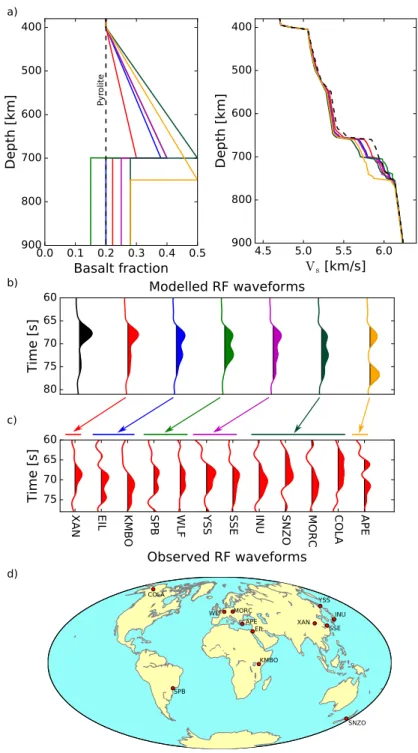
XAN YSS Observed RF waveforms 60 65 70 75 Time [s] APE COLA EIL INU KMBO MORC SNZO SPB SSE WLF XAN YSS a) b) c) d)
Figure 8: Comparison between observed and synthetic receiver function (RF) waveforms computed for different compositional gradients as predicted by mantle convection simulations (e.g., Ballmer et al., 2015). a) Compositional profiles and corresponding shear-wave velocity
tive plate boundaries (e.g., western US or northeast Eurasia), in oceanic regions
366
(e.g., Hawaii and Iceland), and regions of intra-plate volcanism (e.g., Afar) that
367
cannot be explained by a compositionally uniform and adabatic mantle.
Fig-368
ure 8 depicts synthetic RF waveforms computed for different depth-dependent
369
compositional profiles based on predictions from mantle convection simulations
370
(e.g., Tackley, 2008; Ballmer et al., 2015). We find an overall agreement between
371
the observed and synthetic waveforms between 60 and 75 seconds (P660s)
sug-372
gesting that a significant part of the complexity present in the RF waveform data
373
between 60 and 75 seconds (P660s) can be explained by local radial changes in
374
mantle composition. Variations in P660s travel time present in the observed RF
375
waveforms (Figure 8c) most likely reflect local changes in upper mantle
veloc-376
ities due to thermal and compositional variations. Despite being a qualitative
377
comparison, this result supports the existence of local lower-mantle enrichment
378
in basalt (∼5–10% with respect to the upper mantle) and the local
accumu-379
lation of basalt (∼15–30%) in the MTZ. A detailed characterization of these
380
radial changes would require the use of more advanced wave propagation
tech-381
niques (Monteiller et al., 2012) that account for effects introduced by complex
382
three-dimensional structure. Compositional layering has also been found
neces-383
sary to explain regional SS precursors signals beneath Hawaii (Yu et al., 2018)
384
and narrow high-velocity anomalies beneath the MTZ in regions of mantle
up-385
wellings (Maguire et al., 2017). Although the detailed morphology of mantle
386
compositional gradients remains uncertain, all these observations support
geo-387
dynamical simulations that describe mantle convection as a mixture of layered
388
and whole-mantle convection (Tackley, 2000), where cold and/or basaltic
ma-389
terial accumulates above 660 km depth until huge avalanches precipitate it into
390
the lower mantle, “flushing” the local upper mantle through broad cylindrical
391
downwellings to the core-mantle boundary in a globally asynchronous manner
392
(e.g., Tackley, 2008).
5. Conclusions
394
In this paper, we investigated whether compositional mantle stratification
395
is required to jointly explain short- (P-to-s receiver functions) and long-period
396
(Rayleigh wave dispersion) seismic data sensitive to upper mantle and transition
397
zone structure beneath a number of different tectonic settings. This is achieved
398
by implementing a methodology that interfaces the geophysical inversion with
399
self-consistent calculations of mineral phase equilibria on a new global
high-400
quality dataset of receiver function waveforms from an initial pool of 155 stations
401
enhanced with the most recent available global dataset of Rayleigh wave phase
402
velocity dispersion for the fundamental mode and up to fifth overtone.
403
We showed that a compositional boundary is not required to explain
short-404
and long-period seismic data sensitive to the upper mantle and transition zone
405
beneath stable continental regions; yet, radial enrichment in basaltic material
406
reproduces part of the complexity present in the data recorded near
subduc-407
tion zones and volcanically active regions. Our findings further suggest that
408
the mantle is neither completely chemically equilibrated nor fully mechanically
409
mixed, but appears to be best described as an in-between amalgam. In
particu-410
lar, chemical equilibration seems less prevalent beneath cratons suggesting that
411
these regions are possibly isolated from convection processes.
412
Future work will focus on further investigation of the morphology of mantle
413
compositional gradients near subduction zones and volcanically active regions.
414
This will require the incorporation of: 1) a depth-dependent composition and
415
deviations from adiabatic profiles; 2) wave propagation simulations based on
416
more advanced waveform modeling (e.g., Monteiller et al., 2012) to account for
417
three-dimensional effects; and 3) additional information from other geophysical
418
techniques such as Love phase and group velocities (e.g., Khan et al., 2009; Cal`o
419
et al., 2016) or S–to–p converted waves (Oreshin et al., 2008; Yuan et al., 2006)
420
to improve the resolution in the upper mantle.
Acknowledgments
422
We are grateful to John Brodholt and an anonymous reviewer for comments
423
that led to an improved manuscript. This work was supported by the Swiss
424
National Science Foundation (SNSF project 159907). B.T. was funded by the
425
European Union’s Horizon 2020 research and innovation program under the
426
Marie Sklodowska-Curie grant agreement 793824. Calculations were performed
427
using the ETH Zurich cluster Euler.
428
References
429
Anderson, D.L., 2007. New theory of the Earth. Cambridge University Press.
430
Bagheri, A., Khan, A., Al-Attar, D., Crawford, O., Giardini, D., 2019. Tidal
431
response of Mars constrained from laboratory-based viscoelastic dissipation
432
models and geophysical data. Journal of Geophysical Research: Planets
433
doi:10.1029/2019JE006015.
434
Ballard, S., Pollack, H.N., 1987. Diversion of heat by Archean cratons: a model
435
for southern Africa. Earth and Planetary Science Letters 85, 253–264.
436
Ballmer, M.D., Schmerr, N.C., Nakagawa, T., Ritsema, J., 2015. Compositional
437
mantle layering revealed by slab stagnation at ∼1000–km depth. Science
438
advances 1, e1500815.
439
Bernstein, S., Kelemen, P.B., Brooks, C.K., 1998. Depleted spinel harzburgite
440
xenoliths in Tertiary dykes from East Greenland: restites from high degree
441
melting. Earth and Planetary Science Letters 154, 221–235.
442
Boyd, F., Pokhilenko, N., Pearson, D., Mertzman, S., Sobolev, N., Finger, L.,
443
1997. Composition of the Siberian cratonic mantle: evidence from Udachnaya
444
peridotite xenoliths. Contributions to Mineralogy and Petrology 128, 228–246.
445
Cal`o, M., Bodin, T., Romanowicz, B., 2016. Layered structure in the upper
446
mantle across North America from joint inversion of long and short period
447
seismic data. Earth and Planetary Science Letters 449, 164–175.
Carlson, R.W., Pearson, D.G., James, D.E., 2005. Physical, chemical, and
449
chronological characteristics of continental mantle. Reviews of Geophysics
450
43.
451
Cline II, C., Faul, U., David, E., Berry, A., Jackson, I., 2018. Redox-influenced
452
seismic properties of upper-mantle olivine. Nature 555, 355.
453
Cobden, L., Goes, S., Cammarano, F., Connolly, J.A., 2008. Thermochemical
454
interpretation of one-dimensional seismic reference models for the upper
man-455
tle: evidence for bias due to heterogeneity. Geophysical Journal International
456
175, 627–648.
457
Connolly, J., 2009. The geodynamic equation of state: what and how.
Geo-458
chemistry, Geophysics, Geosystems 10.
459
Connolly, J., Khan, A., 2016. Uncertainty of mantle geophysical properties
460
computed from phase equilibrium models. Geophysical Research Letters 43,
461
5026–5034.
462
Cottaar, S., Deuss, A., 2016. Large-scale mantle discontinuity topography
be-463
neath Europe: Signature of akimotoite in subducting slabs. Journal of
Geo-464
physical Research: Solid Earth 121, 279–292.
465
Deuss, A., Andrews, J., Day, E., 2013. Seismic observations of mantle
discon-466
tinuities and their mineralogical and dynamical interpretation. Physics and
467
Chemistry of the Deep Earth , 297–323.
468
Deuss, A., Redfern, S.A., Chambers, K., Woodhouse, J.H., 2006. The nature of
469
the 660-kilometer discontinuity in Earth’s mantle from global seismic
obser-470
vations of PP precursors. Science 311, 198–201.
471
Durand, S., Debayle, E., Ricard, Y., 2015. Rayleigh wave phase velocity and
472
error maps up to the fifth overtone. Geophysical Research Letters 42, 3266–
473
3272.
Efron, B., Tibshirani, R., 1991. Statistical data analysis in the computer age.
475
Science , 390–395.
476
French, S., Romanowicz, B., 2014. Whole-mantle radially anisotropic shear
477
velocity structure from spectral-element waveform tomography. Geophysical
478
Journal International 199, 1303–1327.
479
Frost, D.J., Dolejˇs, D., 2007. Experimental determination of the effect of H2O
480
on the 410–km seismic discontinuity. Earth and Planetary Science Letters
481
256, 182–195.
482
Ghosh, S., Ohtani, E., Litasov, K.D., Suzuki, A., Dobson, D., Funakoshi, K.,
483
2013. Effect of water in depleted mantle on post-spinel transition and
impli-484
cation for 660 km seismic discontinuity. Earth and Planetary Science Letters
485
371, 103–111.
486
Hansen, N., Ros, R., Mauny, N., Schoenauer, M., Auger, A., 2011. Impacts
487
of invariance in search: When CMA-ES and PSO face ill-conditioned and
488
non-separable problems. Applied Soft Computing 11, 5755–5769.
489
Helffrich, G., 2000. Topography of the transition zone seismic discontinuities.
490
Reviews of Geophysics 38, 141–158.
491
Herzberg, C., Asimow, P.D., Arndt, N., Niu, Y., Lesher, C., Fitton, J.,
Chea-492
dle, M., Saunders, A., 2007. Temperatures in ambient mantle and plumes:
493
Constraints from basalts, picrites, and komatiites. Geochemistry, Geophysics,
494
Geosystems 8.
495
Hofmann, A., Hart, S., 1978. An assessment of local and regional isotopic
496
equilibrium in the mantle. Earth and Planetary Science Letters 38, 44–62.
497
Ita, J., Stixrude, L., 1992. Petrology, elasticity, and composition of the mantle
498
transition zone. Journal of Geophysical Research: Solid Earth 97, 6849–6866.
499
Jain, C., Rozel, A., Tackley, P., 2019. Quantifying the correlation between
500
mobile continents and elevated temperatures in the subcontinental mantle.
501
Geochemistry, Geophysics, Geosystems 20, 1358–1386.
Jordan, T.H., 1978. Composition and development of the continental
tecto-503
sphere. Nature 274, 544.
504
Katsura, T., Yoneda, A., Yamazaki, D., Yoshino, T., Ito, E., 2010. Adiabatic
505
temperature profile in the mantle. Physics of the Earth and Planetary
Inte-506
riors 183, 212–218.
507
Khan, A., Boschi, L., Connolly, J., 2009. On mantle chemical and thermal
508
heterogeneities and anisotropy as mapped by inversion of global surface wave
509
data. Journal of Geophysical Research: Solid Earth 114.
510
Khan, A., Connolly, J., Taylor, S., 2008. Inversion of seismic and geodetic
511
data for the major element chemistry and temperature of the Earth’s mantle.
512
Journal of Geophysical Research: Solid Earth 113.
513
Kopylova, M.G., Russell, J.K., 2000. Chemical stratification of cratonic
litho-514
sphere: constraints from the Northern Slave craton, Canada. Earth and
515
Planetary Science Letters 181, 71–87.
516
Lawrence, J.F., Shearer, P.M., 2006a. Constraining seismic velocity and
den-517
sity for the mantle transition zone with reflected and transmitted waveforms.
518
Geochemistry, Geophysics, Geosystems 7.
519
Lawrence, J.F., Shearer, P.M., 2006b. A global study of transition zone thickness
520
using receiver functions. Journal of Geophysical Research: Solid Earth 111.
521
Lenardic, A., Moresi, L., Jellinek, A., O’neill, C., Cooper, C., Lee, C., 2011.
522
Continents, supercontinents, mantle thermal mixing, and mantle thermal
iso-523
lation: Theory, numerical simulations, and laboratory experiments.
Geochem-524
istry, Geophysics, Geosystems 12.
525
Lenardic, A., Moresi, L.N., Jellinek, A., Manga, M., 2005. Continental
insula-526
tion, mantle cooling, and the surface area of oceans and continents. Earth
527
and Planetary Science Letters 234, 317–333.
Ligorria, J.P., Ammon, C.J., 1999. Iterative deconvolution and receiver-function
529
estimation. Bulletin of the seismological Society of America 89, 1395–1400.
530
Maguire, R., Ritsema, J., Goes, S., 2017. Signals of 660 km topography and
531
harzburgite enrichment in seismic images of whole-mantle upwellings.
Geo-532
physical Research Letters 44, 3600–3607.
533
Mattern, E., Matas, J., Ricard, Y., Bass, J., 2005. Lower mantle
composi-534
tion and temperature from mineral physics and thermodynamic modelling.
535
Geophysical Journal International 160, 973–990.
536
McKenzie, D., Bickle, M., 1988. The volume and composition of melt generated
537
by extension of the lithosphere. Journal of petrology 29, 625–679.
538
Monteiller, V., Chevrot, S., Komatitsch, D., Fuji, N., 2012. A hybrid method
539
to compute short-period synthetic seismograms of teleseismic body waves in
540
a 3-D regional model. Geophysical Journal International 192, 230–247.
541
Mosegaard, K., Tarantola, A., 1995. Monte Carlo sampling of solutions to
542
inverse problems. Journal of Geophysical Research: Solid Earth 100, 12431–
543
12447.
544
Muller, G., 1985. The reflectivity method - A tutorial. Journal of
Geophysics-545
Zeitschrift Fur Geophysik 58, 153–174.
546
Munch, F.D., Khan, A., Tauzin, B., Zunino, A., Giardini, D., 2018.
Stochas-547
tic inversion of P-to-s converted waves for mantle composition and thermal
548
structure: Methodology and application. Journal of Geophysical Research:
549
Solid Earth .
550
Murakami, M., Ohishi, Y., Hirao, N., Hirose, K., 2012. A perovskitic lower
551
mantle inferred from high-pressure, high-temperature sound velocity data.
552
Nature 485, 90.
553
Nakagawa, T., Buffett, B.A., 2005. Mass transport mechanism between the
554
upper and lower mantle in numerical simulations of thermochemical mantle
convection with multicomponent phase changes. Earth and Planetary Science
556
Letters 230, 11–27.
557
Oreshin, S., Kiselev, S., Vinnik, L., Prakasam, K.S., Rai, S.S., Makeyeva, L.,
558
Savvin, Y., 2008. Crust and mantle beneath western Himalaya, Ladakh and
559
western Tibet from integrated seismic data. Earth and Planetary Science
560
Letters 271, 75–87.
561
Pearson, D., Canil, D., Shirey, S., 2003. Mantle samples included in volcanic
562
rocks: xenoliths and diamonds. Treatise on geochemistry 2, 568.
563
Ringwood, A., 1975. Composition and petrology of the Earth’s mantle.
564
Ritsema, J., Xu, W., Stixrude, L., Lithgow-Bertelloni, C., 2009. Estimates of
565
the transition zone temperature in a mechanically mixed upper mantle. Earth
566
and Planetary Science Letters 277, 244–252.
567
Rolf, T., Coltice, N., Tackley, P., 2012. Linking continental drift, plate tectonics
568
and the thermal state of the Earth’s mantle. Earth and Planetary Science
569
Letters 351, 134–146.
570
Schaeffer, A., Lebedev, S., 2013. Global shear speed structure of the upper
571
mantle and transition zone. Geophysical Journal International 194, 417–449.
572
Schaeffer, A., Lebedev, S., 2015. Global heterogeneity of the lithosphere and
un-573
derlying mantle: A seismological appraisal based on multimode surface-wave
574
dispersion analysis, shear-velocity tomography, and tectonic regionalization,
575
in: The Earth’s heterogeneous mantle. Springer, pp. 3–46.
576
Schmandt, B., 2012. Mantle transition zone shear velocity gradients beneath
577
USArray. Earth and Planetary Science Letters 355, 119–130.
578
Schulze, K., Marquardt, H., Kawazoe, T., Ballaran, T.B., McCammon, C.,
579
Koch-M¨uller, M., Kurnosov, A., Marquardt, K., 2018. Seismically invisible
580
water in Eearth’s transition zone? Earth and Planetary Science Letters 498,
581
9–16.
Sobolev, A.V., Hofmann, A.W., Kuzmin, D.V., Yaxley, G.M., Arndt, N.T.,
583
Chung, S.L., Danyushevsky, L.V., Elliott, T., Frey, F.A., Garcia, M.O., et al.,
584
2007. The amount of recycled crust in sources of mantle-derived melts. Science
585
316, 412–417.
586
Stixrude, L., Lithgow-Bertelloni, C., 2011. Thermodynamics of mantle
minerals-587
II. Phase equilibria. Geophysical Journal International 184, 1180–1213.
588
Tackley, P.J., 2000. Self consistent generation of tectonic plates in
time-589
dependent, three dimensional mantle convection simulations, part 1:
Pseudo-590
plastic yielding. G3 1.
591
Tackley, P.J., 2008. Geodynamics: Layer cake or plum pudding? Nature
592
Geoscience 1, 157.
593
Tauzin, B., Debayle, E., Wittlinger, G., 2008. The mantle transition zone as
594
seen by global Pds phases: no clear evidence for a thin transition zone beneath
595
hotspots. Journal of Geophysical Research: Solid Earth 113.
596
Thio, V., Cobden, L., Trampert, J., 2015. Seismic signature of a hydrous mantle
597
transition zone. Physics of the Earth and Planetary Interiors 250, 46–63.
598
Wang, F., Barklage, M., Lou, X., van der Lee, S., Bina, C.R., Jacobsen, S.D.,
599
2018. HyMaTZ: a Python program for modeling seismic velocities in hydrous
600
regions of the mantle transition zone. Geochemistry, Geophysics, Geosystems
601
19, 2308–2324.
602
Wu, W., Ni, S., Irving, J.C., 2019. Inferring Earth’s discontinuous chemical
603
layering from the 660–kilometer boundary topography. Science 363, 736–740.
604
Xu, W., Lithgow-Bertelloni, C., Stixrude, L., Ritsema, J., 2008. The effect of
605
bulk composition and temperature on mantle seismic structure. Earth and
606
Planetary Science Letters 275, 70–79.
607
Yu, C., Day, E.A., Maarten, V., Campillo, M., Goes, S., Blythe, R.A., van der
608
Hilst, R.D., 2018. Compositional heterogeneity near the base of the mantle
609
transition zone beneath Hawaii. Nature Communications 9, 1266.
Yuan, X., Kind, R., Li, X., Wang, R., 2006. The S receiver functions: synthetics
611
and data example. Geophysical Journal International 165, 555–564.
Supplementary material for online publication only