HAL Id: hal-02130490
https://hal.archives-ouvertes.fr/hal-02130490
Submitted on 23 May 2020
HAL is a multi-disciplinary open access
archive for the deposit and dissemination of
sci-entific research documents, whether they are
pub-lished or not. The documents may come from
teaching and research institutions in France or
abroad, or from public or private research centers.
L’archive ouverte pluridisciplinaire HAL, est
destinée au dépôt et à la diffusion de documents
scientifiques de niveau recherche, publiés ou non,
émanant des établissements d’enseignement et de
recherche français ou étrangers, des laboratoires
publics ou privés.
Dual-primal skeleton: a thinning scheme for vertex sets
lying on a surface mesh
Ricardo Uribe Lobello, Jean-Luc Mari
To cite this version:
Ricardo Uribe Lobello, Jean-Luc Mari. Dual-primal skeleton: a thinning scheme for vertex sets lying
on a surface mesh. 14th International Symposium on Mathematical Morphology (ISMM 2019), Jul
2019, Saarbrücken, Germany. �10.1007/978-3-030-20867-7_6�. �hal-02130490�
for vertex sets lying on a surface mesh
Ricardo Uribe Lobello* and Jean-Luc Mari
Aix Marseille Universit´e, Universit´e de Toulon, CNRS, LIS, Marseille, France
Abstract. We present a new algorithm for the skeletonization of shapes lying on surface meshes, which is based on a thinning scheme with a gran-ularity that is twice as fine as that of other thinning methods, since the proposed approach uses dual-primal iterations in the region of interest to perform the skeleton extraction. This dual operator is built on specific construction rules, and it is applied until idempotency, which provides a better geometric positioning of the skeleton compared to other thin-ning methods. Moreover, the skeleton has the property of ensuring the same topological guarantees as other homotopic thinning approaches: the skeleton is thin, connected and can include Y-branches and cycles if the input region contains holes.
Keywords: skeletonization, surface mesh, homotopic thinning, shape de-scription, topology preservation.
1
Introduction
1.1 Context, problem and related work
The skeleton is a well-known shape descriptor. It is an entity that is globally centered in a 2D or 3D object, and it characterizes its topology and its geometry. This structure is widely used in various applications (video tracking [4], shape recognition [13], surface sketching [9], etc.). Several techniques exist in order to extract the skeleton from binary 2D images [14], 3D closed volume meshes [2], or 3D cubic grids [8].
Nevertheless, very few approaches have been dedicated to the extraction of skeletons from binary information located on an arbitrary triangulated mesh (see [3,12,11] for the state of the art). Therefore, the task of computing the skeleton of the subset of a discrete surface embedded in R3 remains. R¨ossl et al. [10] have presented the first method that uses the elementary mathemati-cal morphology opening operator, ported to triangulated meshes. However, the operator’s definition is incomplete, and the underlying algorithm presents some issues. Therefore, several drawbacks have been pointed out, which mainly lead to unexpectedly disconnected skeletons [5]. Kudelski et al. have later proposed a modified algorithm that produces topologically robust skeletons by generaliz-ing the notion of morphological erosion to arbitrary meshes [7,6]. This approach takes, as an input, a subset lying on a triangulated surface mesh in 3D, and as
outputs, thin lines corresponding to the skeleton obtained by homotopic thin-ning. The main idea is to transpose the notion of neighborhood from the classical thinning algorithms where the adjacency is constant (e.g., 26-adjacency in digital volumes, 8-adjacency in 2D grids) to the mesh domain where the neighborhood is variable due to the adjacency of each vertex.
1.2 Contribution
Our work continues the idea of homotopic thinning using a generalized adjacency described in [6]. Instead of iteratively removing nonrelevant vertices of the subset (topologically speaking, i.e., the simple vertices), the erosion step is replaced by a dual-primal operation. The area of interest is converted to the dual space, and all semi-infinite edges are removed from the structure. This process is repeated (dual to primal to dual) until idempotency. It produces a lineal skeleton with a resolution increased by a factor 2, as the resulting structure is not only composed of initial vertices and edges but also composed of dual vertices and edges. This skeletonization is more general because it can address nondevelopable surfaces (the operations are local, and there is no need to have a [i, j] indexing such as in 2D grids). Moreover, the resulting skeleton preserves the topology of the original shape lying on the surface.
This paper is divided as follows: section 2 briefly develops some basic notions and definitions. Then, section 3 explains in detail our approach of dual-primal skeletonization using a specific thinning scheme on surface meshes. Section 4 is dedicated to the validation of the method, including tests on irregular meshes and an application to the extraction of feature lines.
2
Basic notions
Let M be an unstructured mesh patch representing an arbitrary manifold sur-face S, such as M = (V, E , T ). The sets V, E and T correspond, respectively, to the vertices, the edges, and the triangles composing M, a piecewise linear approximation of S. We denote pi the vertices, with i ∈ [0; n[ and n = |V| being
the number of vertices in M. The neighborhood N of a vertex pi is defined as
follows:
N (pi) = {qj | ∃ (pi, qj) ∈ E }. (1)
In such a case, mi= |N (pi)| represents the total number of neighbors of pi.
As we consider obtaining a skeleton of a subset of M, let us now define a binary attribute F on each vertex of V. The set R ⊆ V is then written as follows:
∀pi ∈ R ⇐⇒ F (pi) = 1. (2)
The attribute F may be defined from a previous process such as manual selection, thresholding based on geometric properties (triangle area, principal curvatures, etc.) or any binarization process. Then, an edge e = (p, q) belongs to R if and only if p, q ∈ R. Similarly, a triangle t = (p, q, r) belongs to R if and only if p, q, r ∈ R.
3
Dual-primal skeletonization
Our approach is based on a robust dual-primal erosion algorithm that preserves the topology of the original mesh. In the next sections, we present an overview of our algorithm and a detailed explanation of each part of our algorithm.
3.1 Overview of the approach
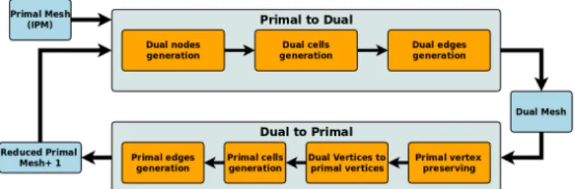
The input to our algorithm can be any triangular mesh M that is a set of trian-gular faces connected by edges and vertices as defined in section 2. As in section 2, this mesh must have the vertices marked with a function in order to define re-gions of interest. M can contain several connected components, and it can have one or several borders. Hereafter, we will call the input mesh the initial primal mesh (IPM). Our approach is straightforward; it starts by extracting the dual representation of the IPM. Then, it detects the faces that can be eliminated by exploring the dual mesh. Finally, it computes the intermediate primal represen-tation of the mesh by eliminating the primal faces that are not going to affect the topology of the final skeleton. Then, we repeat the dual-primal iteration over this new primal mesh. Finally, it stops when the primal mesh in iteration N is equal to the primal mesh in iteration N+1. The main steps of our approach are illustrated in figure 1.
Fig. 1: General structure of the workflow of our approach. The initial mesh is provided as input. A dual representation is computed. Then, a primal mesh is obtained by eliminating those dual cells that are not totally contained in the areas of interest. The new primal mesh can contain edges representing the thin features of the input mesh. Finally, the reduced mesh is provided as input to the next iteration until idempotency.
The primal-to-dual and dual-to-primal transformations are performed by fol-lowing a well-defined set of rules that guarantee that the final mesh will preserve the topology of the IPM.
3.2 Primal-Dual-Primal computation
In classic dual extraction algorithms, the dual mesh is extracted based on an edge adjacency relationship between cells. For each edge in the primal mesh,
a dual edge is generated. However, this narrow definition is not sufficient to obtain a 1-dimensional skeleton because it does not consider vertex adjacencies between edges and vertex adjacency between faces. Vertex adjacency is necessary to detect all connected components in the area of interest in the original mesh. Furthermore, as our algorithm applies an erosion to the input mesh, it will eventually lead to the creation of mixed meshes containing 2-dimensional (faces) and 1-dimensional (edges) cells that are uniquely connected by vertices. Our approach addresses these cases in order to keep the consistency and fidelity of the final mesh with respect to the IPM.
3.3 General rules for dual mesh generation
These rules follow classic definitions of dual meshes extracted from polygonal meshes.
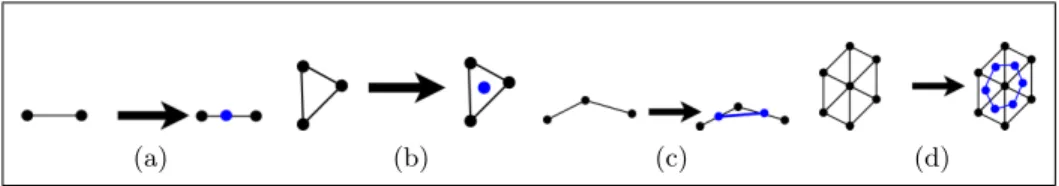
1. Each primal cell is replaced by a dual vertex. It includes primal faces and primal edges. Initially, we always place the dual vertex in the barycenter of the primal cell as illustrated in figures 2a and 2b.
2. Each primal vertex is replaced by a dual cell. In the case of vertices sur-rounded by 2-dimensional cells, the dual cell is a polygon. In the case of a vertex surrounded by edges, it is replaced by a dual edge. These cases are illustrated in figures 2c and 2d.
(a) (b) (c) (d)
Fig. 2: Basic transformations from a primal mesh to a dual mesh. (a) Primal edge to dual vertex. (b) Primal face to dual vertex. (c) Primal vertex to dual edge. (d) Primal vertex to dual cell (a polygon).
As a consequence of the previous rules, starting from a primal mesh Mk =
{V, E, C}, its dual mesh Dk = {Vd, Ed, Cd} (in the general case) is defined by
equations:
Vd= {vdi| ∃ci∈ C so that vdiis located at the barycenter of fi} (3)
Ed= {edi| ∃ei∈ E} (4)
Cd= {cdi| ∃vi∈ V} (5)
These definitions apply, as mentioned, in the general case of a closed mesh without borders. The IPM can have borders, and thus, the intermediate meshes
can contain borders. Therefore, the previous definitions have to be expanded to consider these special cases. For example, the region R can contain thin structures; hence, it is not possible to generate the classic dual cell, but it is possible to generate linear dual cells. We will explain these cases in more detail in the next section.
3.4 Generation of dual cells in particular cases
To address all possible cases in a region with borders and to prove its topological correctness, it is necessary to expand our definition of a dual mesh.
Dual vertex generation Our algorithm simply traverses each cell in the primal mesh M and computes a dual vertex placed in the barycenter of the current cell. This algorithm is easily applied over 1-dimensional and 2-dimensional cells. There is no need to extend the current definitions.
Dual cell generation In the general case, it is possible to build the dual cell di around a primal vertex ci by extracting its face neighborhood as defined in
equation 6
Nf(ci) = {fj| ci ∈ V(fj) where V(fj) is the set of vertices of cell fj}. (6)
From Nf(ci), it is possible to generate the dual vertices that will be connected
to generate the dual cell. However, it is necessary to ensure that the faces are ordered counterclockwise in order to obtain a well oriented dual mesh. To do this, our algorithm extracts the ordered neighborhood of the primal vertices around ciby traversing all faces incidents to ci. Then, we extract all edges in those faces
not containing ci. Finally, we order these edges to create a closed path. This
algorithm only works in well oriented surfaces. Thus, this vertex neighborhood can be redefined as follows.
Nv(ci) = {cj ∈ V(fk) | ∃fk∈ Nf(ci) and cj6= ci}. (7)
The vertices contained in Nv(ci) can be ordered to check if the current vertex
ciis actually surrounded by a closed path of vertices. If it is the case, it is possible
to generate the dual cell. If it is not the case, the current vertex belongs to a thin structure or a border. Our algorithm to process these cases will be explained in the next section.
It is necessary to also handle the cases where 1-dimensional and 2-dimensional cells are adjacent. In these cases, it is necessary to make a decision about the way how these cells have to be connected, which occurs in both the primal space and in the dual space, and the method used to solve this is presented in the next section.
3.5 Handling mixed regions
Mixed regions usually appear when large components encounter thin structures. It can happen in the transition from primal to dual and in the dual-to-primal transformation. Therefore, we develop these two transitions separately.
Primal to Dual Transformation Once the dual vertices have been generated, it is necessary to detect thin structures to avoid the separation of components connected by a strip of triangles or a set of vertices. To detect if a primal face f is contained in a thin structure, we traverse each of its primal vertices checking if a ring can be built around each one. If this is not possible for any of them, this primal face is marked as comprising part of a thin structure. Then, each dual vertex in every face is connected to the dual vertex in the edge-adjacent cell in order to generate a dual edge. This process is repeated until all dual vertices in the thin structure are connected. It is important to clarify that edges generated in thin structures are 1-dimensional dual cells and are stored explicitly, in contrast to edges comprising part of 2-dimensional dual cells, which are stored implicitly. This process is illustrated in figure 3.
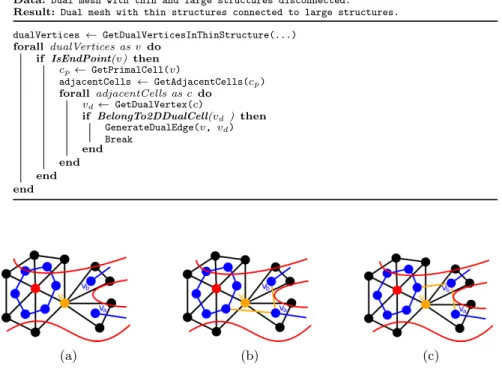
Fig. 3: Detection of thin structures. For each primal vertex, we check the 1-ring built from its incident faces. In red, a primal vertex in a larger structure. In yellow, these primal vertices do not have a 1-ring around them. Consequently, all primal faces containing only these kinds of vertices are part of a thin structure. In blue are dual vertices, dual faces and dual edges.
As seen in figure 3, dual vertices in thin structures are still not connected to dual vertices in the larger structure. Our algorithm traverses all dual vertices belonging to thin structures to detect end points, which is done by checking if the dual vertex is only adjacent to one 1-dimensional cell. Then, for each end point vendpoint, we obtain its primal cell cp, and we check if cp is an edge-adjacent
to another primal cell ca so that it contains a dual vertex belonging to a
2-dimensional dual cell. We do this only once in order to avoid connecting the thin structure with the larger structure multiple times. This procedure is listed in the algorithm 1.
As mentioned previously, our algorithm connects vertex-adjacent regions in order to preserve the topology of a region of interest defined with marked ver-tices, which is implemented in the primal-to-dual phase. Dual vertices in vertex-adjacent primal vertices are always connected by an edge. It is important to remember that a primal cell can be edge-adjacent to several structures. Conse-quently, it is necessary to detect all components that have to be connected with the current dual vertex, which is illustrated in figure 4a.
To connect these structures, it is necessary to detect one of the end points va or vb. Then, the algorithm extracts the set of primal cells C that are adjacent
to the shared primal vertex v. Next, we extract the connected components of C. Finally, we choose one of the primal cells belonging to each connected component
Algorithm 1: Connecting the dual vertices in a thin structure with the dual vertices in larger structures.
Data: Dual mesh with thin and large structures disconnected. Result: Dual mesh with thin structures connected to large structures.
dualVertices ← GetDualVerticesInThinStructure(...) forall dualVertices as v do if IsEndPoint(v) then cp← GetPrimalCell(v) adjacentCells ← GetAdjacentCells(cp) forall adjacentCells as c do vd← GetDualVertex(c) if BelongTo2DDualCell(vd) then GenerateDualEdge(v, vd) Break end end end end (a) (b) (c)
Fig. 4: In red, we illustrate potential borders for the structure approximated by the area of interest. (a) Vertex-adjacent components in the Dual cells and dual vertices are in blue. The large structure is composed of a dual cell in blue. This structure is connected to two thin structures by the primal vertex in orange. (b) The three components are connected by the orange edges from va. It is clear,
however, that we can obtain different meshes depending on the initial dual vertex (c). As explained later, we do not consider this as a limitation for our approach because the topology of the area of interest is preserved.
that contains a dual vertex, and we connect va (or vb) with each one of these
dual vertices. This procedure is listed in algorithm 2 and illustrated in figure 4b. By using this method, it is possible to obtain different meshes from the same input depending on the dual vertex that is first detected (va or vb). However,
as this choice does not change the topology (but the connectivity) of the final mesh. As our objective is to preserve the topology in the sense of connected components, holes and voids and not in terms of connectivity of the mesh, this result is correct.
Dual-to-Primal Transformation Once a dual mesh has been generated, our approach detects which primal cells can be eliminated without affecting the topology of the final linear structure. To do this, we apply the following rule:
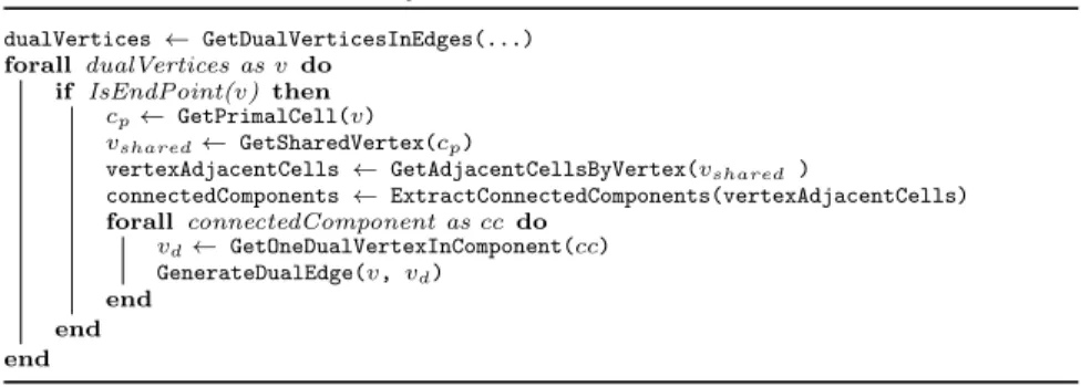
Algorithm 2: Connecting the dual vertices of vertex-adjacent primal cells. This algorithm can connect multiple dual vertices from multiple vertex-adjacent primal cells (see figure 4).
Data: Dual mesh with vertex-adjacent structures disconnected. Result: Dual mesh with vertex-adjacent structures connected.
dualVertices ← GetDualVerticesInEdges(...) forall dualVertices as v do
if IsEndPoint(v) then cp← GetPrimalCell(v)
vshared← GetSharedVertex(cp)
vertexAdjacentCells ← GetAdjacentCellsByVertex(vshared )
connectedComponents ← ExtractConnectedComponents(vertexAdjacentCells) forall connectedComponent as cc do vd← GetOneDualVertexInComponent(cc) GenerateDualEdge(v, vd) end end end
Rule 1 A primal cell must be preserved if and only if its dual vertex is shared by three 2D dual cells.
The rule 1 is intended to preserve primal cells that are part of large structures. This rule also implies that all primal cells corresponding to a dual vertex shared uniquely by one or two 2D dual cells must be eliminated. These primal cells are, evidently, always located in the frontiers of the structure. Therefore, the application of rule 1 results in an erosion of the larger structures from the border to the inside, similar to the prairie fire algorithm used in topological thinning methods. It is implemented by traversing all dual vertices and obtaining its adjacent dual cells.
(a) (b) (c) (d)
Fig. 5: General illustration of the transition from dual to primal. This example shows a large structure connected to a thin structure.
The rule 1 is only intended to preserve interior faces. The connectivity be-tween large and thin structures is represented as a dual edge sharing a dual vertex with a 2-dimensional dual cell, as explained in the previous section. To preserve this topology in the next primal mesh, we proceed as follows. In the case of primal faces belonging to thin structures and, as consequence, represented in the dual mesh by dual vertices, they are not preserved; however, each one is replaced by its dual vertex, which is added to the next primal mesh. Dual edges inside these thin structures are all preserved as primal edges. Finally, dual edges connecting to 2-dimensional dual cells are also preserved by adding the shared
dual vertex to the primal vertices and connecting it to the primal vertex at the origin of the primal 2-dimensional cell.
This process is illustrated in figure 5 with the original mesh in black and the initial dual mesh in blue. In figure 5b, green faces and vertices are preserved, all primal faces and vertices that are going to be eliminated (by using the comple-ment of rule 1) are in red. In 5c, thin and large structure are still not connected. In 5d, These structures are connected by using the primal vertex at the origin of the 2-dimensional dual cell and the dual vertex in the same dual cell connected to the thin structure.
The method previously described is sufficiently general to address several thin structures or branches converging toward a single 2-dimensional dual cell and can generate multiple junctions at the same point; it preserves the topology of the original area of interest.
As evident from the primal mesh obtained in figure 5d, our approach generates intermediary meshes that are a mixture of faces and edges as illustrated in figure 6a. Therefore, this kind of configuration has to be addressed in the primal-to-dual transition. In these cases, the algorithm connects the primal-to-dual vertex in the primal edge with the dual vertex belonging to the adjacent primal face, forming a junction as shown in figure 6b.
(a) (b)
Fig. 6: General illustration of the extraction of a dual mesh in areas of the mesh where primal faces and edges are connected. (a) This primal mesh has been generated from a previous iteration. It generates mixed meshes with edges and faces. (b) The dual mesh in blue is generated mostly by using the standard rules explained earlier. However, in mixed areas, dual vertices in edges have to be connected to dual vertices in primal faces generating a junction.
The previous primal-to-dual and dual-to-primal processes are applied itera-tively until idempotency. In this final stage, we obtain a mesh containing edges only. These edges are positioned approximately at the center of the topological structures of the original area of interest. This fact will help to better understand the next section.
3.6 Geometric positioning
The algorithm generates linear meshes well positioned in the center of the main structures of the original object, which is possible because of the symmetrical erosion procedure that is used to progressively eliminate the most external primal faces in the mesh. As explained above, our algorithm advances from the borders of the mesh to the interior. Thus, the final structure converges slowly towards the center of the structure. Additionally, we use the primal vertices if possible;
however, if necessary, we generate and add dual vertices to the next primal mesh. These dual vertices are placed in the barycenter of primal faces, thus increasing the centering of the final structure, especially in thin structures.
Concerning the geometric position with respect to the original surface, we use, if possible, the original primal vertices. If dual vertices are used in the final mesh, they are strictly located over the primal faces. Therefore, the vertices of the final mesh are always located over the original mesh. By contrast, final edges are not always located on the surface. It is only the case when the edge is relying two initial primal meshes. In any other case, all the points of the edge are not necessarily on the surface.
3.7 Topological guarantees
The topological guarantees offered by our approach can be proven by analyzing the different cases that can appear in the primal-to-dual and dual-to-primal transitions.
Lemma 1. In the transition from the primal mesh to the dual mesh, all topo-logical structures are represented through their dual counterparts.
Proof. Let Ap = {Vp, Fp, Ep} with Vp be a set of primal vertices, Fp be a set
of primal faces and Ep be a set of edges. We consider Sp a conformal mesh so
that N-dimensional cells only intersect on (N-1)-dimensional cells. Triangles only intersect in an edge or a vertex and edges only intersect in a vertex. Therefore, we consider that Ap is also conformal.
First, let the dual mesh be defined equivalently as Ad = {Vd, Fd, Ed}. As our
algorithm generates one dual vertex for each primal cell or edge, we find that the set of dual vertices Vd is composed of dual vertices centered at their
corre-sponding primal cell, as illustrated in figure 2a and 2b. Hence, each face fpi∈ Fp
or edge ei
p ∈ Ep in the region Ap is represented by a dual vertex vdi ∈ Vd.
Uniform regions : In the case of 2 edges connected by a primal vertex, dual vertices are connected by a dual edge (see 2c). In the case of primal vertices surrounded by faces, dual vertices are connected as illustrated in figure 2d. This construction guarantees that linear structures will still be represented by linear (but dual) structures. In the case of triangulations, they will be represented by at least one dual cell.
Mixed regions : these are regions where a triangulation representing a large structure Lp is connected to a thin structure Tp by at least a primal vertex.
These thin structures can be a strip of triangles or a set of edges. Two cases can be considered:
– If Lp∪ Tp is an edge: The dual vertices belonging to the edge-adjacent
triangles are connected by a dual edge, thus connecting the two regions. – If Lp∪ Tp is a primal vertex: Lp and Tp are either two primal faces or a
primal face and a primal edge. Then, the dual vertex in Tpis connected to the
first primal cell of each vertex-adjacent connected component as illustrated in figure 4.
Mixed regions in the primal mesh only transform into dual edges in the dual mesh. As we have assumed that the area of interest is a conformal surface, the cases explained above connect all cells that are at least connected by a primal vertex. Consequently, this algorithm preserves the topology of the original surface.
Lemma 2. In the transition from the dual mesh to the primal mesh, all topo-logical structures are preserved.
Proof. To prove lemma 2, we need to proceed by case:
– Dual edges: Dual edges are only converted to primal edges. Therefore, thin structures are preserved.
– Large structures: As mentioned previously, all internal dual vertices are transformed to primal cells. All noninternal dual vertices and their corre-sponding primal faces are eliminated. If no internal dual vertices exist, it means it is a thin structure; in any other case, primal faces will be con-served, and this structure will be present in the next iteration.
– Mixed structures: A 2-dimensional dual cell connected to a dual edge. In this case, the connection between the components is always conserved because the primal vertex at the center of the dual edge will be connected to the primal vertex at the origin of the 2-dimensional dual cell.
In conclusion, no components that have been connected during the primal-to-dual process are separated in the primal-to-dual-to-primal transition. All connections are preserved in the edge and vertex adjacency. Consequently, the topology of the original region of interest is preserved.
3.8 Post-processing
Pruning Our algorithm uses a simple criterion to eliminate parasite branches. It consists of the detection of ending vertices of the structure. For each of these ending vertices, it checks if it belongs to the original mesh. If this is the case, this branch is preserved because it can represent an important feature of the region. If the ending vertex does not belong to the initial mesh, it means that it has been created during the primal-dual-primal iteration process. In this case, it is not sure that the vertex reflects a thin structure in the initial mesh. In this article, we have decided to keep these branches if they have a minimum length (a parameter) but more research is needed to establish if they really have to be conserved.
Smoothing As our approach is based entirely on the geometrical information of the mesh, it can produce highly oscillating structures. To improve these re-sults, we apply a simple smoothing algorithm that moves every vertex to the barycenter of the vertices composing its topological neighborhood similar to the ”Beatifying” algorithm proposed in [1].
Evidently, as this process can affect the approximation quality of the final skele-ton, we bound the maximum approximation error from the original mesh.
4
Results and validation
These results have been obtained in the Ubuntu 16.04 LTS 64-bit environment with the processor, Intel i7-7820HQ CPU @ 2.90 GHz × 8 and 32 GBytes of internal memory. It has been implemented in C++, and the mesh data structure used was the vtkPolyData. We used VTK built-in methods to traverse the mesh and access to its properties. Our approach is intended to work in 2-dimensional simplex meshes that can be mapped in 3D in order to represent volumes. For this, we have started applying it to 2D planar meshes and the results are discussed in the next section.
4.1 Application on planar meshes
In figure 7, our implementation is applied to four different meshes. These meshes are regular meshes with relatively well-formed faces. In the figure, we show the original mesh and the extracted skeleton after cleaning and some iterations of the smoothing process. Table 1 shows relevant information about the examples presented in figure 7.
(a) Cross. (b) Shape. (c) Letter A. (d) Letter B. Fig. 7: Application of our algorithm to 2D meshes. The cleaned skeleton is shown after a smoothing process.
Table 1: Information on the execution of the algorithm in the four previous planar meshes. This table shows the number of primal-to-dual and dual-to-primal iterations, the execution time and the total number of edges in the final skeleton.
Data set # Triangles # Iterations Exec. Time (in ms) Lines Final skeleton
Cross 819 5 246 108
Shape 8556 13 4529 1009
A letter 812 6 261 103
B Letter 4307 9 2049 361
From figure 7, it is clear that the algorithm is able to extract skeletons from arbitrary triangular meshes while preserving the topology of the original mesh. It keeps junctions and holes, and places the final skeleton at approximately the center of the topological structure. However, the method is entirely based on the geometry and the connectivity of the mesh, and consequently, a different triangulation of the same object will produce a different skeleton.
Concerning the execution time, our implementation is not optimal because of the choice of the vtkPolyData structure. The vtkPolyData depends on a loga-rithmic data structure to traverse neighboring cells and adjacent vertices. Having
into account the vtkPolyData data structure, the complexity of the dual vertex generation process is O(NK1(F + V )) and including the complexity of the dual cell generation, the final complexity of our method is O(N [K1[(F +V )+V log F ]). As seen, the execution time of our algorithm is highly dependent of the size and connectivity of the input mesh. As optimization and with a half-edge data struc-ture, the k1V log F part of our approach can be optimized to a constant factor.
4.2 Application on surfaces
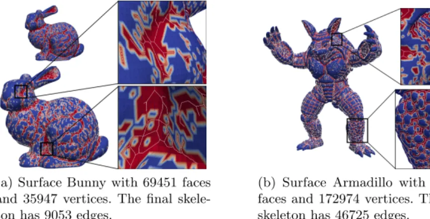
We have applied our approach to surfaces mapped in 3D that represent volumes. These surfaces have to be marked in order to define areas of interest. In figure 8, we show two surface meshes where areas of maximum curvature are marked. Our approach has extracted skeletons close to the center of interest areas.
(a) Surface Bunny with 69451 faces and 35947 vertices. The final skele-ton has 9053 edges.
(b) Surface Armadillo with 345944 faces and 172974 vertices. The final skeleton has 46725 edges.
Fig. 8: Application to the high curvature areas of a surface (in red). Two closeups show how the skeleton (in white) is located in the middle of the region of interest.
As seen in figure 8, our algorithm is robust enough to be applied to any 2D mesh with complex topology. It is able to connect connected components with edge and vertex connectivity, allowing us to preserve the topology of thin structures connected only by 1-dimensional cells or edges. However, our current implementation does not guarantee that the skeleton is located in the center of the connected component but tends to place it close to it. To offer guarantees on the location of the skeleton, it will likely be necessary to follow closely the position of dual vertices, thus minimizing its distance to the center of mass of the current component. This kind of implementation can be used to extract the main features of surface meshes in the future.
5
Conclusion and future work
We have tested our approach and we have confirmed that the algorithm is robust and capable of extracting a 1-dimensional structure from any region lying on a mesh with arbitrary topology. However, this approach is highly dependent on
the size and connectivity of the mesh. Thus, we think that a more efficient mesh data structure can strongly improve the complexity and the execution time of our method.
As future work, we consider that our approach is not limited to 2D triangular meshes, and it can be easily extended to simplicial meshes in higher dimensions.
References
1. Carlo Arcelli and Gabriella Sanniti di Baja. Euclidean skeleton via centre-of-maximal-disc extraction. Image and Vision Computing, 11(3):163 – 173, 1993. 2. Oscar Kin-Chung Au, Chiew-Lan Tai, Hung-Kuo Chu, Daniel Cohen-Or, and
Tong-Yee Lee. Skeleton extraction by mesh contraction. ACM Transaction on Graphics, 27(3):1–10, August 2008.
3. Thomas Delame, Jacek Kustra, and Alexandru Telea. Structuring 3d medial skele-tons: A comparative study. In Symposium on Vision, Modeling and Visualization, 2016.
4. J. Gall, C. Stoll, E. De Aguiar, C. Theobalt, B. Rosenhahn, and H.P. Seidel. Motion capture using joint skeleton tracking and surface estimation. In IEEE Computer Society Conference on Computer Vision and Pattern Recognition (CVPR’09), pages 1746–1753. IEEE Computer Society, June 2009.
5. Dimitri Kudelski, Jean-Luc Mari, and Sophie Viseur. Extraction of feature lines with connectivity preservation. In Computer Graphics International (CGI’11 elec-tronic proceedings), June 2011.
6. Dimitri Kudelski, Sophie Viseur, and Jean-Luc Mari. Skeleton extraction of vertex sets lying on arbitrary triangulated 3D meshes. In Discrete Geometry for Computer Imagery - 17th IAPR International Conference, DGCI 2013, Seville, Spain, March 20-22, 2013. Proceedings, pages 203–214, 2013.
7. Dimitri Kudelski, Sophie Viseur, Giovanni Scrofani, and Jean-Luc Mari. Feature line extraction on meshes through vertex marking and 2D topological operators. Int. J. Image Graphics, 11(4):531–548, 2011.
8. T.C. Lee, R.L. Kashyap, and C.N. Chu. Building skeleton models via 3-D me-dial surface/axis thinning algorithms. Graphical Models and Image Processing, 56(6):462–478, November 1994.
9. Jean-Luc Mari. Surface sketching with a voxel-based skeleton. In 15th IAPR International Conference on Discrete Geometry for Computer Imagery (DGCI’09), volume 5810 of Lecture Notes in Computer Science, pages 325–336. Springer, 2009. 10. Christian R¨ossl, Leif Kobbelt, and Hans-Peter Seidel. Extraction of feature lines on triangulated surfaces using morphological operators. In AAAI Spring Symposium on Smart Graphics, volume 00-04, pages 71–75, March 2000.
11. Punam K Saha, Gunilla Borgefors, and Gabriella Sanniti di Baja. A survey on skeletonization algorithms and their applications. Pattern Recognition Letters, 76:3–12, 2016.
12. Andrea Tagliasacchi, Thomas Delame, Michela Spagnuolo, Nina Amenta, and Alexandru Telea. 3d skeletons: A state-of-the-art report. In Computer Graph-ics Forum, volume 35, pages 573–597. Wiley Online Library, 2016.
13. Kai Yu, Jiangqin Wu, and Yueting Zhuang. Skeleton-based recognition of chinese calligraphic character image. In Advances in Multimedia Information Processing (PCM’08), volume 5353 of Lecture Notes in Computer Science, pages 228–237. Springer, 2008.
14. T. Y. Zhang and C. Y. Suen. A fast parallel algorithm for thinning digital patterns. Communications of the ACM, 27(3):236–239, March 1984.