HAL Id: hal-02018634
https://hal-amu.archives-ouvertes.fr/hal-02018634
Preprint submitted on 14 Feb 2019
HAL is a multi-disciplinary open access
archive for the deposit and dissemination of
sci-entific research documents, whether they are
pub-lished or not. The documents may come from
teaching and research institutions in France or
abroad, or from public or private research centers.
L’archive ouverte pluridisciplinaire HAL, est
destinée au dépôt et à la diffusion de documents
scientifiques de niveau recherche, publiés ou non,
émanant des établissements d’enseignement et de
recherche français ou étrangers, des laboratoires
publics ou privés.
Modeled With Labeled Petri Nets Using an Overall
Fault Status
Guanghui Zhu, Lei Feng, Zhiwu Li, Naiqi Wu
To cite this version:
Guanghui Zhu, Lei Feng, Zhiwu Li, Naiqi Wu. Online Fault Diagnosis of Discrete Event Systems
Modeled With Labeled Petri Nets Using an Overall Fault Status. 2018. �hal-02018634�
Online Fault Diagnosis of Discrete Event Systems
Modeled With Labeled Petri Nets Using an Overall
Fault Status
Guanghui Zhu, Student Member, IEEE, Lei Feng, Zhiwu Li, Fellow, IEEE, Naiqi Wu, Senior Member, IEEE
Abstract—In this paper we present a fault diagnosis approach using labeled Petri nets, where the faults are modeled by unobservable transitions and the unobservable subnet is acyclic. In contrast to detecting the individual faults separately, a new specification called an overall fault status is introduced, which in-dicates the occurrence of faults from a global system perspective. Due to the introduction of the overall fault status, a more precise and informative diagnosis result can be provided and in some cases, the occurrence of some faults in a system can be detected before the actual faults are isolated, i.e., we are certain about the occurrence of faults but which faults have not been ascertained. An integer linear programming (ILP) problem is built according to the observed word. We prove that all transition sequences determined by solutions to the ILP problem constitute the set of sequences consistent with the observed word. By specifying different objective functions to the ILP problem, the diagnosis results of each individual fault and the overall fault status can be obtained. An online diagnosis algorithm is developed to implement the proposed diagnosis process, which reports the diagnosis results after the occurrence of every observable event.
Index Terms—Fault diagnosis, discrete event system, Petri net, integer linear programming, overall fault status.
I. INTRODUCTION
A. Position of the paper
With the development of contemporary information technol-ogy, the man-made mechanical and electronic systems that can be characterized as discrete event systems (DES) are becoming more and more complicated. To ensure their stable and correct operations, fault diagnosis has been an active research area in recent decades. A fault is a kind of event that causes a deviation in system’s behavior such that the performance or throughput of the system is degraded. Fault diagnosis aims to detect and isolate a fault when it occurs such that it can be fixed and the system can recover from it.
This work was supported in part by the National Natural Science Foundation of China under Grant Nos. 61873342 and 61703321, in part by the Science and Technology Development Fund, MSAR, under Grant Nos. 122/2017/A3 and 106/2016/A3, and in part by the 2017 Sino-French Cai Yuanpei Program. (Corresponding author: Zhiwu Li.)
G. Zhu is with the School of Electro-Mechanical Engineering, Xidian Uni-versity, Xi’an 710071, China, and with Aix Marseille UniUni-versity, Universite de Toulon, CNRS, LIS, Marseille, France (e-mail: [email protected]). L. Feng is with the Department of Machine Design, KTH Royal Institute of Technology, 100 44 Stockholm, Sweden (e-mail: [email protected]).
Z. Li is with the School of Electro-Mechanical Engineering, Xidian University, Xi’an 710071, China, and also with the Institute of Systems Engineering, Macau University of Science and Technology, Taipa, Macau (e-mail: [email protected]).
N. Wu is with the Institute of Systems Engineering, Macau University of Science and Technology, Taipa, Macau (e-mail: [email protected]).
The diagnosis of discrete event systems was originally discussed in [1], [2] using an automaton model with faulty (unobservable) events, where a diagnoser, i.e., a deterministic finite automaton (DFA), is first built and then based on the observed sequence the diagnosis result can be directly obtained by checking the diagnoser. The authors also define the diagnosability of an automation model and provide a necessary and sufficient condition for diagnosability.
An alternative to automata for modeling DES is provided by Petri nets. Their structural properties offer a new perspective for supervisory control [3], [4], model identification [5], [6], performance optimization [7], and knowledge discovery [8], [9]. In addition, the state equation of a Petri net provides a linear algebraic technique to deal with the issue of state estimation [10]–[14], which is always more efficient than exhaustively enumerating the reachability graph. In particular, we in this paper deal with the fault diagnosis issue using Petri nets.
In the context of Petri nets, Prock [15] proposed a diagnosis approach for a nuclear power plant by monitoring the number of tokens residing in places associated with P-invariants in a Petri net. Wu and Hadjicostis [16] developed an algebraic approach for fault diagnosis, where both place and transition faults are defined. By introducing additional places into a net, a redundant Petri net can be obtained. The place and/or transition faults can be detected by inspecting the current marking of the redundant net. Ram´ırez-Trevi˜no et al. [17] proposed a modeling methodology to build an interpreted Petri net (IPN) model of a system and then a fault detection algorithm based on the built IPN is provided. Benveniste et al. [18] reported a net unfolding approach to explore the diagnosis of asynchronous systems, which can be used in a distributed environment.
On the other hand, there is a deluge of studies that use Petri nets by explicitly modeling faults of a system as un-observable transitions [19], i.e, Petri nets, called faulty Petri nets, that contain not only regular but faulty behavior of a system. Genc et al. [20] originally extended the event-based diagnosis using automata to the case of faulty Petri nets. They construct a diagnoser, i.e., a labeled Petri net, according to the original net model of a system and a diagnosis result can be provided online when observing an event. The main drawback of this approach is the computational complexity due to the reachability analysis at each step. Giua and Seatzu
[21] proposed a basis-marking-based approach. By means
enumeration of paths in a reachability graph can be avoided. Cabasino et al. [22]–[24] extended this approach to the case of labeled Petri nets, i.e., nets where two or more transitions can share the same label. They develop a basis reachability graph (BRG), which can be built off-line and provides an efficient method for online diagnosis. In [25], Basile et al. defined a new type of marking with negative elements, called g-marking, and proposed an online diagnosis algorithm based on it. Integer linear programming (ILP) is a typical technique to deal with the issue of state estimation in a Petri net. An online diagnosis approach using ILP is reported in [26]. More specifically, the authors first build an integer linear programming model without objective function according to the observed transition sequence. Then, by assigning different objective functions to it, the occurrence of a fault can be detected. Ru et al. [27] addressed the issue of fault diagnosis using a partially observed Petri net (POPN), where a POPN is first converted into a labeled net and then an algorithm based on the reachability graph is proposed.
t1(a) t3 p1 p3 p2 p5 p4 p7 p6 t2 t5(b) t6 2 2 p8 t9 t11(c) f1 f2 t8(a) t7(b) t10(b) t4(c) p9 p10 p11 3 f3 t12(d)
Fig. 1. A plant model producing bolts and nuts.
B. Motivation
In a faulty Petri net model, faults are explicitly modeled as unobservable transitions and the transition set T is divided into two disjoint subsets Toand Tu with T = To∪ Tu, where
To denotes the set of observable transitions and Tu the set of
unobservable transitions. Transitions t1∈ To and t2∈ Tu are
assigned a label from the event set E and an empty string ε, respectively. In general, the diagnosis result provided by approaches based on faulty Petri nets [12], [21]–[23], [25], [28] can be represented by a function ∆ : E∗×Tf → {0, 1, 2},
where E is the set of events associated with a faulty net, Tf = {f1, . . . , fnf} ⊆ Tu is the set of nf fault transitions,
and 0, 1 and 2 denote that fault transition fi ∈ Tf does not
occur for sure, fi may occur and fi occurs with certainty,
re-spectively. For example, assuming that the observed sequence is ω, ∆(ω, f1) = 1 indicates that f1 may (possibly) occur till
the observation of ω.
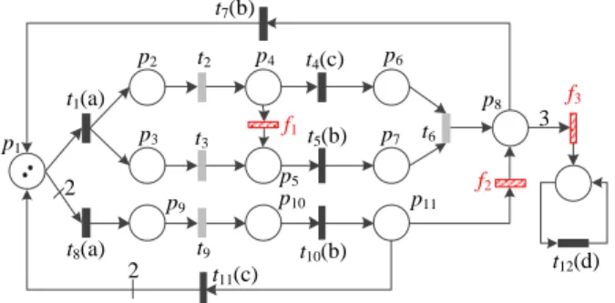
We next provide an example to show the motivation of introducing an overall fault status. Consider the net in Fig. 1
that models a plant producing bolts and nuts. This plant has two production lines: one (upper part) produces mini-size bolts and nuts and the other (lower part) produces
medium-size ones. In Fig. 1, we have E = {a, b, c, d}, Tu =
{t2, t3, t6, t9, f1, f2, f3}, Tf = {f1, f2, f3}, Ta = {t1, t8},
Tb = {t5, t7, t10}, Tc = {t4, t11}, and Td = {t12}. The
unobservable transitions are represented as gray bars (fault transitions f1, f2 and f3 are colored red), and Tx denotes
the set of transitions labeled x with x ∈ {a, b, c, d}. It is significant to design an algorithm to solve the following problem.
Problem 1. Consider the net shown in Fig.1and assume that the observed sequence is ω = abb. Does the plant modeled by this net run normally till the observation of ω? (i.e., have some faults occurred in the plant?)
The existing approaches for fault diagnosis, such as those in [12], [21], [23], [25], [28], provide an ambiguous answer to Problem1only. The procedure in [23], [25], [28] to solve Problem1 can be summarized as follows.
Step 1: Compute the diagnosis results of f1, f2 and f3,
re-spectively, and obtain that ∆(ω, f1) = 1, ∆(ω, f2) =
1, and ∆(ω, f3) = 0.
Step 2: Because of the ambiguous diagnoses of f1 and f2,
one cannot unambiguously determine the occurrence of faults and only an answer that the plant may run abnormally can be provided.
In fact, the exact answer is that the plant runs abnormally and one of f1 and f2 necessarily occurs. This situation can
be explained by Fig. 2(a), where the symbol ε denotes an
empty string. As a part of reachability graph of the net shown in Fig.1, it shows all transition sequences consistent with ω. In Fig. 2(a), M0 is the initial marking, and Mω1 and Mω2
are the markings reachable by firing the sequences consistent with ω = abb. We observe that each path from M0to Mω1or
Mω2 either goes through f1 or f2, i.e., there is no path that
passes none of faults. Fig.2(a) can be condensed as Fig.2(b) which shows all the paths more intuitively. By considering all possible evolutions of the plant consistent with the observation abb, there does not exist a possibility that no fault occurs since each path contains a fault transition. This implies that a fault must occur till the observation of abb and the plant does not run normally. t1(a) t8 (a) t2(e ) t3(e ) t3(e) f1 t2(e) t5(b) t2(e) f1 t3(e) t5(b) t3(e) f1 t5(b) t5(b) t5(b) t9(e) t10(b) f2 t7(b) M0 Mw1 Mw2 f1 f1 f1 f2 M0 Mw1 Mw2 (a) (b)
Fig. 2. (a) All paths consistent with abb and (b) an intuitive representation of (a).
This paper will provide a more precise and informative
solution to Problem 1 by extending the existing diagnosis
function. The new diagnosis function is defined as ∆ : E∗× TfS → {0, 1, 2}, where TfS = Tf∪ {F } and F stands for
the overall fault status. In contrast to detecting the individual fault separately, the overall fault status indicates the occurrence of faults from a global system perspective. In particular, ∆(ω, F ) = 0 denotes that a system is running normally, ∆(ω, F ) = 1 some faults may occur in the system, and 2 some faults must have occurred. Note that, in some cases, the diagnosis of F , i.e., ∆(ω, F ), can be directly inferred from ∆(ω, fi) with i = 1 . . . nf. However, in other cases, novel
methodologies have to be proposed to compute ∆(ω, F ). Due to the use of the overall fault status, in some cases, one can detect the occurrence of faults before the actual faults are isolated. Let us consider the net in Fig.1again. The diagnosis results for observed words ω’s are listed in Table I, where ∆(ω, F ) denotes the diagnosis of the overall fault status.
We observe that for ω = a, both f1 and f2 do not occur.
For ω = abb, both f1 and f2 may occur, as indicated by
∆(abb, f1) = 1 and ∆(abb, f2) = 1. However, ∆(abb, F ) = 2
implies that at least one fault must occur in the plant even if the diagnoses of f1 and f2are ambiguous, i.e., we detect the
occurrence of faults before the definite diagnosis of individual fault transition.
TABLE I
DIAGNOSIS RESULTS FOR OBSERVED WORDω.
f ∆(ω, f ) ω a ab abb . . . abbacba f1 0 1 1 . . . 2 f2 0 0 1 . . . 0 f3 0 0 0 . . . 0 F 0 1 2 . . . 2
This is particularly meaningful for a system that needs to respond to failures in time. For example, consider an aircraft with five faults from f1 to f5. If we detect that
∆(ω, f1) = 1, ∆(ω, f2) = 1, ∆(ω, fi) = 0 for i = 3, . . . , 5,
and ∆(ω, F ) = 2, some faults must occur in the aircraft though we cannot determine which faults occur at present. The captain of the aircraft can deal with this situation immediately before an unambiguous fault is reported.
However, for systems that can tolerate failures, we can wait for a longer observation of an event sequence in order to exactly find the faults with less cost. For example, some components of a system are hard to access and one should exactly identify the location of a fault before taking any corrective action that may involve component inspection and replacement [2]. If the occurrence of faults in a system is detected according to the overall fault status F and the exact faults cannot be currently ascertained, we can consider the following two ways to find the exact faults:
(1) Observe continuously the output of a net till a sufficiently long sequence is observed if the net is diagnosable (see SectionV);
(2) Stop the real-world system and inspect all the faults f ’s with ∆(ω, f ) = 1 one by one.
The first way provides exact fault locations such that they can be fixed in a short time. But a long wait may be needed to precisely identify the faults. For example, considering Fig. 1
and TableI, we detect the occurrence of faults (∆(abb, F ) = 2) but cannot determine that the fault is f1 or f2 when ω =
abb. If the plant continues to run and the observed word is
ω = abbacba, we then conclude that fault f1 must happen
(∆(ω, f1) = 2) and f2 not (∆(ω, f2) = 0). On the other
hand, for the second way, one has to stop (part of) the plant and further test it to find the faulty components. This will possibly reduce the throughput of the plant and increase the cost of isolating faults.
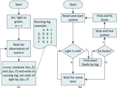
When performing diagnosis in a system, we will first try to detect any abnormal behavior of the system based on the observation. If the behavior is found to be abnormal, we will refine the diagnosis by using new observations and possibly further testing the system until the faulty components are found [29]. In this paper, a framework to isolate and fix faults in a system is proposed based on the overall fault status F . This framework is appropriate for faults that cause significant changes in the system state but do not bring the system to a halt. In a real-world system, the overall fault status F can be viewed as a fault indicator light that has three colors of green (∆(ω, F ) = 0), yellow (∆(ω, F ) = 1), and red (∆(ω, F ) = 2). If the light is green, it implies that the system is running normally and no fault is detected. Whereas a red light indicates that one or more faults have occurred and then one can check ∆(ω, fi) with i = 1, . . . , nf to localize and fix
the faults. Graphically, the diagnosis flow can be described by Fig.3. Start Set light to green, w = e Wait for observation of event e w=we, compute D(w, fi)
and D(w, F) and write to running log, set color of
light by D(w, F) Running log example: a b c f1 0 0 1 f2 0 1 1 F 0 1 2 Start Reset and start
system
Light is red?
Wait for some time
Fix faults? Stop and test
system Find and fix
faults N N Y Y (a) (b) Find exact faults by log
Fig. 3. (a) Diagnosis process and (b) supervision process
As shown in Fig.3, there are two processes in the system: diagnosis process and supervision process. The diagnosis process makes a diagnosis when observing an event and enters the diagnosis result into a log file (see Fig.3(a)). Note that a plant may continue to run and record the diagnosis result even if some faults have occurred. The supervision process monitors
the operation of the plant and decides whether to stop it to fix faults when the indicator light is red (see Fig. 3(b)).
C. Contribution
In this paper, we extend the approach in [26] to explore an improved diagnosis algorithm based on labeled Petri nets and the overall fault status. As done in the literature [22], [25], the approach in [26] can only be used for a special class of labeled Petri nets, i.e., nets in which each observable transition is assigned a unique label. We first extend the approach in [26] to the case of a labeled Petri net with an arbitrary labeling function, i.e., two or more transitions can share the same label, and then propose some new theoretical results to compute ∆(ω, F ). An online diagnosis approach is presented, which implements the diagnosis process described in Fig. 3(a).
Note that Fanti et al. [30] also extend the approach in [26] to the case of a labeled Petri net. They first build an ILP problem based on a transition sequence σo∈ To∗ using a special class
of labeled Petri net where an observable transition is assigned
a unique label. Then, for an observed word ω ∈ E∗, they
exhaustively enumerate all possible sequences σo’s with σo∈
To∗ whose projections on E are ω and, for each sequence
σo, solve a number of ILP problems built from it to perform
online diagnosis. For an observed word ω, there may exist a lot of transition sequences σo’s whose projection on E are
ω. Thus, a large number of ILP problems may need to be solved according to the approach in [30], which is infeasible in general due to prohibitive computational cost.
Different from the work in [30], we in this paper extend and improve the approach in [26] from a different perspective. Specifically, our extension is completely based on labeled Petri nets and an ILP problem is constructed based on the observed word ω not a transition sequence σo ∈ To∗. Compared with
the approach in [30], the number of times of solving ILP problems of our approach is usually considerably small when perform diagnosis for an observed word (see Section VI for an example).
The main contributions of the paper can be summarized as follows.
(1) We introduce a new diagnosis specification called an overall fault status and extend the diagnosis function such that a more precise and informative diagnosis result can be provided.
(2) We extend and improve the approach in [26] to the case of general labeled Petri nets, i.e., nets where two or more transitions can share the same label. Different from the extension in [30], we do not need to enumerate all possible sequences of observable transitions consistent with an
observed word ω ∈ E∗ and just solve an ILP problem
built according to ω to perform diagnosis.
(3) In contrast to the work in [30], our approach is usually more efficient, demonstrated by extensive experimental studies (see SectionVI).
This paper is organized in seven sections. We in Sec-tion I review the related literature and show the motivation of introducing the overall fault status. The basic definitions and preliminaries on Petri nets are recalled in Section II.
Section IIIdefines the problem on which this paper focuses. In SectionIV, a solution based on integer linear programming
is proposed. Section V discusses the relationship between
the diagnosability and the overall fault status. We present an example to compare the proposed approach with the one in [30] in Section VI. Finally, we conclude the paper in SectionVII.
II. PRELIMINARIES
This section recalls the Petri net formalism and some preliminary results used throughout the paper. The readers can refer to [31] and [32] for more details on Petri nets. We denote by N the set of non-negative integers.
A. Basics of Petri nets
A Petri net is a four-tuple N = (P, T, P re, P ost), where P = {p1, . . . , pm} is a set of m places, T = {t1, . . . , tn}
is a set of n transitions with P ∪ T 6= ∅ and P ∩ T = ∅, P re : P × T → N and P ost : P × T → N are the pre-and post-incidence matrices, respectively, which specify the structure of the net. Graphically, places and transitions are represented by circles and bars, respectively. For each arc with weight γ from place p (transition t) to transition t (place p), it holds P re(p, t) = γ (P ost(p, t) = γ). The other elements of P re and P ost are 0. The incidence matrix of a net is denoted by C = P ost − P re. A Petri net is said to be acyclic if there is no directed cycle.
For a transition t ∈ T , its preset is defined as •t = {p ∈ P | P re(p, t) > 0}, and its postset is defined as t• = {p ∈ P | P ost(p, t) > 0}. A transition t is said to be a source transitionif•t = ∅.
A marking of a Petri net is a vector M : P → N, and M (p) indicates the number of tokens, pictorially denoted by black dots, in place p. We use x1p1+ · · · + xmpm to denote the
marking [x1, . . . , xm]T for economy of space. A net system
hN, M0i is a Petri net N with an initial marking M0.
A transition t ∈ T is enabled at marking M if for all p ∈
•t, M (p) ≥ P re(p, t), which is denoted by M [ti. An enabled
transition t at M can fire yielding a new marking M0 such that M0= M + C(·, t), which is denoted by M [tiM0.
For a transition sequence σ ∈ T∗and a marking M , M [σi denotes that σ is enabled at marking M and M [σiM0 denotes that a new marking M0 is reachable from M after firing σ. The set of all the markings reachable from M0 is denoted by
R(N, M0), called the reachability set of a Petri net. The set
of transition sequences enabled at the initial marking M0 is
defined as
L(N, M0) = {σ ∈ T∗| M0[σi}
which is called the language of Petri net system hN, M0i.
We define a function π : T∗ → Nn that maps a transition
sequence σ ∈ T∗ to n-dimensional column vector y = π(σ),
called firing vector, such that y(t) = k if transition t appears k times in σ. Write t ∈ σ to denote that t is contained in σ.
Given M0[σiM , we have
Eq. (1), called the state equation, shows that there exists a
non-negative integer vector y such that M = M0+ C · y
if M is reachable from M0, which is a necessary but not
sufficient condition for the reachability of marking M from M0. However, for an acyclic net, it is necessary and sufficient,
as verified by the following result.
Theorem 1. [31] Let hN, M0i be an acyclic Petri net. A
marking M ≥ 0 is reachable from M0 if and only if (iff)
there exists a non-negative integer vector y satisfying M = M0+ C · y.
B. Labeled Petri net
Given a Petri net N = (P, T, P re, P ost) and the event set E, a labeling function λ : T → E ∪ {ε} assigns to each transition t ∈ T either a symbol from the event set E or an empty string ε. In the case of no confusion, a labeled Petri net in this paper refers to a net with an arbitrary labeling function, i.e., two or more transitions can share the same label. A Petri net system hN, M0i with a labeling function λ : T → E ∪ {ε}
is called a labeled Petri net system, denoted by hN, M0, E, λi.
A transition t is said to be unobservable or silent if it is associated with the label ε, i.e., λ(t) = ε. The set of unob-servable transitions is denoted by Tu = {t ∈ T | λ(t) = ε}
with cardinality nu. All other transitions whose labels come
from event set E constitute the set of observable transitions
To = {t ∈ T | λ(t) 6= ε} with cardinality no. Thus,
set T is divided into two disjoint subsets To and Tu with
T = To∪ Tu. For a faulty Petri net, the faults are always
modeled by unobservable transitions and accordingly the set of unobservable transitions is also divided into two disjoint subsets Treg and Tf, i.e., Tu= Treg∪ Tf, where Treg denotes
the set of regular unobservable transitions and Tf the set of nf
fault transitions. We use Te= {t ∈ T | λ(t) = e} to represent
the set of transitions with the same label e ∈ E.
Analogous to the definition of function π, for each sequence σo ∈ To∗, we define a function πo: To∗ → Nno such that
y = πo(σo) and y(t) = k if t ∈ To appears k times in σo.
Similarly, the function πu: Tu∗→ Nnu associates a sequence
σu∈ Tu∗ with an nu-dimensional vector πu(σu).
We extend the definition of labeling function λ to a sequence
σt ∈ T∗ such that λ(σt) = λ(σ)λ(t), i.e., for a sequence
σ ∈ T∗, ω = λ(σ) is an observed word composed of the labels of observable transitions contained in σ. The set of observed words in a labeled Petri net system hN, M0, E, λi is defined
as
LE(N, M
0) = {ω ∈ E∗| σ ∈ L(N, M0), ω = λ(σ)}.
Given a transition sequence σ, we use ←−σ to denote the last transition in σ. For example, if σ = t1t2t3, we have←σ = t− 3.
For an observed word ω ∈ LE(N, M0), the set
C(ω) = {σ ∈ T∗| σ ∈ L(N, M0), λ(σ) = ω}
denotes all sequences that are consistent with ω and ←−
C (ω) = {σ ∈ T∗| σ ∈ C(ω), ←σ ∈ T− o}
stands for the consistent transition sequences whose last tran-sitions are observable, i.e., the sequences with observable tails.
Accordingly, the set of markings that are reachable by firing the consistent transition sequences with observable tails is defined as
←−
D (ω) = {M ∈ Nm| σ ∈←−C (ω), M
0[σiM }.
Example 1. Consider the net shown in Fig. 1 and a
part of its reachability graph shown in Fig. 2. If the
observed word is ω = a, then it is readily verified
that C(ω) = {t1, t1t2, t1t2f1, t1t2f1t3, t1t2t3, t1t2t3f1, t1t3,
t1t3t2, t1t3t2f1, t8, t8t9} and
←−
C (ω) = {t1, t8}. On the other
hand, for ω = abb, we have ←D (ω) = {M− ω1, Mω2}.
Definition 1. Given a net N = (P, T, P re, P ost) and a subset of transitions T0⊆ T , the T0-induced subnet of N is a Petri
net N0= (P, T0, P re0, P ost0), where P re0 and P ost0 are the restrictions of P re and P ost to P × T0, respectively, i.e., the net N0 is obtained by removing all transitions in T \ T0 from N .
Given a net N = (P, T, P re, P ost) with T = To∪ Tu,
according to Definition 1, one can readily obtain from N the observable subnet No = (P, To, P reo, P osto) and the
unobservable subnet Nu = (P, Tu, P reu, P ostu). Moreover,
the incidence matrices of nets No and Nu are denoted by
Co= P osto− P reo and Cu = P ostu− P reu, respectively.
Note that, as in the literature [22], [25], [26], this paper assumes that the unobservable subnet is acyclic.
III. PROBLEMSTATEMENT
Fault diagnosis consists in determining if faults have oc-curred in a system according to the observed system output, such as the observed word ω in a Petri net. As done in the literature, we can design a diagnoser, i.e., a diagnosis function, to show the diagnosis result. For a labeled Petri net with event set E, a diagnoser is a function ∆ : E∗× Tf → {0, 1, 2} such
that a fault f ∈ Tf does not occur if ∆(ω, f ) = 0, may occur
if 1, and necessarily occurs if 2. Next, we provide the formal definition of diagnosis function ∆.
Definition 2. Let hN, M0, E, λi be a labeled Petri net system.
The diagnosis function ∆ : E∗× Tf → {0, 1, 2} associates an
observed word ω ∈ LE(N, M0) and a fault f ∈ Tf with a
diagnosis state such that
(1) ∆(ω, f ) = 0 if for all σ ∈←−C (ω), f /∈ σ, i.e., each path consistent with ω in the reachability graph does not pass fault transition f .
(2) ∆(ω, f ) = 1 if there exist σ1, σ2 ∈
←−
C (ω) such that f /∈ σ1 and f ∈ σ2, i.e., there exist two paths, one of which
passes f and the other does not.
(3) ∆(ω, f ) = 2 if for all σ ∈←−C (ω), f ∈ σ.
Note that some existing studies [21], [22] additionally consider the possible fault transitions after the last observed event of ω when performing diagnosis, i.e., the definition of ∆ is based on C(ω) not ←−C (ω). However, we in this paper do not adopt this setting and detect only the fault transitions occurring before the last event of ω in order to be consistent with the seminal work in [1].
From Definition 2, we observe that the diagnoser ∆ only concerns if an individual fault f ∈ Tf has occurred during
the system evolution and there is no information to indicate the overall system fault state, i.e., the diagnosis results of all fault transitions cannot completely describe the fault state of the system. To overcome this, we introduce the notion of the overall fault status F in Subsection I-B.
A diagnostic Petri net system hN, M0, E, λ, F i is a labeled
Petri net system hN, M0, E, λi with an overall fault status F .
For hN, M0, E, λ, F i, the diagnosis function is extended as
∆ : E∗ × TfS → {0, 1, 2}, where TfS = Tf ∪ {F }. The
diagnosis of F is defined as follows.
Definition 3. Let hN, M0, E, λ, F i be a diagnostic Petri net
system. For an observed word ω ∈ LE(N, M
0), the diagnosis
of F is represented by a diagnosis function ∆ : E∗× TfS →
{0, 1, 2} such that
(1) ∆(ω, F ) = 0 if for all σ ∈ ←−C (ω) and for all f ∈ Tf,
f /∈ σ.
(2) ∆(ω, F ) = 1 if there exist σ1, σ2∈
←−
C (ω) such that (i) for all f ∈ Tf, f /∈ σ1 and (ii) there exists f ∈ Tf, f ∈ σ2.
(3) ∆(ω, F ) = 2 if for all σ ∈ ←−C (ω), there exists f ∈ Tf
such that f ∈ σ.
In some cases, the value of ∆(ω, F ) can be directly de-duced from ∆(ω, fi). We provide the following proposition
to formalize this situation. However, when there exist two or more f ’s such that ∆(ω, f ) = 1, we have to figure out a new method to compute ∆(ω, F ).
Proposition 1. Given a diagnostic Petri net system
hN, M0, E, λ, F i and an observed word ω ∈ LE(N, M0), the
following statements hold:
(1) ∆(ω, F ) = 0 if for all f ∈ Tf, ∆(ω, f ) = 0,
(2) ∆(ω, F ) = 2 if there exists f ∈ Tf such that ∆(ω, f ) = 2,
(3) ∆(ω, F ) = 1 if there exists only one f ∈ Tf such that
∆(ω, f ) = 1 and ∆(ω, f0) = 0 for other faults f0 ∈ T f.
Proof. The conclusions (1) and (2) can be directly derived from Definitions 2 and3. For (3), since there is one f ∈ Tf
such that ∆(ω, f ) = 1, there exist two paths σ1, σ2 ∈
←− C (ω) satisfying f ∈ σ1 and f /∈ σ2. Moreover, for any other fault
transition f0, it holds ∆(ω, f0) = 0. Thus, we have f /∈ σ2
for each f ∈ Tf, i.e., ∆(ω, F ) = 1.
The conclusion (3) in Proposition1 provides a straightfor-ward method to compute ∆(ω, F ) in the case that there is only one f ∈ Tf satisfying ∆(ω, f ) = 1 (for all f0 ∈ Tf \ {f },
∆(ω, f0) = 0). However, for the case that there are two or more f ’s such that ∆(ω, f ) = 1, Corollary 3 has to be em-ployed to compute ∆(ω, F ). The Lines14–19of Algorithm1
show the use of Proposition 1 when performing diagnosis of F .
Next, we formally define the problem considered in this paper. In Section IV, an algorithm based on integer linear programming is provided to solve this problem.
Problem 2 (Online diagnosis). Given a diagnostic Petri net system hN, M0, E, λ, F i with T = To∪ Tu and Tu= Treg∪
Tf, let the observed word ω be null initially. The diagnosis
problem consists in computing ∆(ω, f ) and ∆(ω, F ) for each observed event e during the evolution of the system, where ω = ωe, f ∈ Tf, and F is the overall fault status.
By Definitions2and3, we know that an intuitive method to solve Problem2 is to analyze the reachability graph of a net. However, this is usually infeasible because of its huge size. In order to avoid analyzing the reachability graph, an integer linear programming technique is often used for a Petri net. We next present an ILP-based solution to Problem2.
IV. ILP-BASED SOLUTION
In [26], an approach based on ILP is proposed for fault diagnosis using Petri nets in which each observable transition is associated with a unique label. In this paper, we introduce the overall fault status and extend this approach to the case of a labeled Petri net. First, we give a theorem that is the cornerstone of the proposed ILP-based approach.
Theorem 2. Given a labeled Petri net hN, M0, E, λi and an
observed word ω = e1e2. . . eh ∈ LE(N, M0), there exists a
sequence σ = σu1tα1. . . σuhtαh ∈
←−
C (ω) if and only if there exist vectors yiand binary variables zjeiwith i = 1, . . . , h and
j = 1, . . . , nei satisfying the following equation
M0+ Cu· i X γ=1 yγ+ i−1 X γ=1 neγ X δ=1 C(·, teγ δ ) · (1 − z eγ δ ) − P re(·, tei 1) ≥ −z ei 1 · K .. . M0+ Cu· i X γ=1 yγ+ i−1 X γ=1 neγ X δ=1 C(·, teγ δ ) · (1 − z eγ δ ) − P re(·, tei nei) ≥ −zneiei · K zei 1 + . . . + z ei nei = nei− 1 Tei = {t ei 1 , . . . , teniei} yi∈ Nnu zei 1, . . . , zeniei ∈ {0, 1} i = 1, . . . , h, (2) where h ∈ N is the length of the observed word, nei is the
cardinality of set Tei, σui∈ T
∗
u, tαi ∈ Tei, yi= πu(σui) is a
firing vector, and K is a sufficiently large positive integer. Proof. For i = 1, . . . , h, Eq. (2) contains h groups of con-straints.
(if ) For i = 1, we obtain the first group of constraints shown as follows: M0+ Cu· y1− P re(·, te11) ≥ −z e1 1 · K .. . M0+ Cu· y1− P re(·, tne1e1) ≥ −zne1e1· K ze1 1 + . . . + zne1e1 = ne1− 1 Since ze1
k with k = 1, . . . , ne1 are binary variables, there must
exist a variable with value 0 among them. Without loss of generality, we assume ze1
1 = 0. Then we have M0+ Cu·
y1≥ P re(·, te11). Considering that the unobservable subnet is
acyclic, there exists a transition sequence σu1 ∈ T
∗
y1= πu(σu1) and M0[σu1t e1 1 i. It is clear that σu1t e1 1 ∈ ←− C (e1) holds.
For i = 2, we obtain the second group of constraints: M0+Cu· (y1+ y2) + C(·, te11)(1 − z e1 1 ) + . . . + C(·, te1 ne1)(1 − z e1 ne1) − P re(·, t e2 1 ) ≥ −z e2 1 · K .. . M0+Cu· (y1+ y2) + C(·, te11)(1 − z e1 1 ) + . . . + C(·, te1 ne1)(1 − z e1 ne1) − P re(·, t e2 ne2) ≥ −z e2 ne2· K ze2 1 + . . . + zne2e2 = ne2− 1 We know that ze1 1 = 0 and z e1 k = 1 with k = 2, . . . , ne1.
More-over, analogous to the situation of i = 1, we assume ze2
1 = 0.
Thus, we have M0+ Cu· y1+ C(·, t1e1) + Cu· y2≥ P re(·, te12).
Since there exists a sequence σu1 satisfying M0[σu1t
e1
1 iM1
and y1= πu(σu1), M1+Cu·y2≥ P re(·, t
e2
1 ) holds. Being the
unobservable subnet acyclic, there exists σu2 ∈ T
∗
u such that
M1[σu2t
e2
1 i and y2 = πu(σu2). Thus we conclude that there
exists σ = σu1t
e1
1 σu2t
e2
1 satisfying M0[σi and σ ∈
←− C (e1e2).
If the theorem is true for i = k − 1 with 2 ≤ k ≤ h, we next prove that it holds for i = k. For i = k, without loss of generality, we assume zej 1 = 0 with j = 1, . . . , k. Then, it holds M0+ Cu· k X γ=1 yγ+ k−1 X γ=1 C(·, teγ 1 ) ≥ P re(·, t ek 1 ).
Moreover, we have already known that yi = πu(σui)
with i = 1, . . . , k − 1 and M0[σu1tα1. . . σuk−1tαk−1iMk−1.
Thus, Mk−1 + Cu · yk ≥ P re(·, te1k) ≥ 0 holds.
S-ince the unobservable subnet is acyclic, there exists a
se-quence σuk ∈ T ∗ u such that Mk−1[σukt ek 1 iMk. Thus, it holds σu1tα1. . . σuk−1tαk−1σuktαk ∈ ←− C (e1. . . ek), i.e., we
prove by induction that there exists a sequence σ =
σu1tα1. . . σuhtαh ∈
←− C (ω).
(only if ) For the observed word ω = e1e2. . . eh, if there
exists a sequence σ = σu1tα1. . . σuhtαh ∈
←−
C (ω), a solution to Eq. (2) can be found as follows. First, we set yi= πu(σui)
for i = 1, . . . , h. Second, since tαi ∈ Tei, without loss of
generality, we assume tei
1 = tαi and then it holds z
ei
1 = 0 and
zei
i = 1 for i = 2, . . . , nei. Thus, there exist yi and z
ei
j with
i = 1, . . . , h and j = 1, . . . , nei satisfying Eq. (2).
On the basis of Theorem2, we can infer that all sequences σ’s corresponding to the solutions to Eq. (2) constitute the set ←−C (ω). Thus, by associating an objective function with Eq. (2), we can determine if a fault has occurred or not. In the following, three corollaries based on Theorem2 are provided to describe this.
Corollary 1. Given a labeled Petri net hN, M0, E, λi and
an observed word ω = e1e2. . . eh, then for each f ∈ Tf,
∆(ω, f ) = 0 if ILPP 1 admits a solution γ = 0. ILPP 1: γ = max h P i=1 yi(f ) s.t. Eq. (2)
Proof. If γ = 0, by checking all possible solutions to Eq. (2), there does not exist yi such that yi(f ) > 0. By Theorem 2,
each σui in σ = σu1tα1. . . σuhtαh ∈
←−
C (ω) does not contain f , i.e., for all σ ∈ ←−C (ω), f /∈ σ, which implies ∆(ω, f ) = 0.
Corollary 2. Given a labeled Petri net hN, M0, E, λi and an
observed word ω = e1e2. . . eh, for each f ∈ Tf, ∆(ω, f ) = 2
if ILPP 2 admits a solution γ > 0.
ILPP 2: γ = min h P i=1 yi(f ) s.t. Eq. (2)
Proof. If γ > 0, then there exists at least one yi in solutions
to Eq. (2) such that yi(f ) > 0, i.e., for all σ ∈
←−
C (ω), f ∈ σ, which indicates ∆(ω, f ) = 2.
For an observed word ω and each f ∈ Tf, Corollaries1and
2are devoted to computing the value of ∆(ω, f ). On the other hand, for the overall fault status F , we can compute ∆(ω, F ) according to Proposition1 and the following corollary.
Corollary 3. Given a diagnostic Petri net system
hN, M0, E, λ, F i and an observed word ω = e1e2. . . eh,
∆(ω, F ) = 2 if ILPP 3 admits γ > 0 and ∆(ω, F ) = 0 or 1 if γ = 0. ILPP 3: γ = min ~11×nf · h P i=1 yi(Tf) s.t. Eq. (2) Proof. Note that objective function Ph
i=1yi(Tf) denotes the
sum of projections of nu-dimensional column vectors yi’s over
the set Tf. If γ = 0, there exists a group of unobservable
sequences σui corresponding to yi with i = 1 . . . h such that
σ = σu1tα1. . . σuhtαh and f /∈ σ for each f ∈ Tf, i.e., there
exists at least one path which passes none of fault transitions in the reachability graph from M0 to
←−
D (ω). Thus, in this case, ∆(ω, F ) = 0 or 1 according to Definition 3. On the contrary, if γ > 0, there does not exist such a path, i.e., each path must pass one or more fault transitions. Thus, we have ∆(ω, F ) = 2.
Now, an online algorithm to Problem 2 can be provided.
Algorithm1describes the basic steps of how to perform diag-nosis in a labeled Petri net by using the ILP technique only. The correctness of this algorithm is ensured by Proposition1
and Corollaries1,2 and3.
We briefly illustrate how Algorithm1works. It is described in C-like syntax. For example, we use the symbol “=” to represent an assignment operation and “==” to indicate that
two variables are equal. In Line 1, R = ~0nf is an n
f
-dimensional column vector that records the diagnosis result of each f ∈ Tf. For a fault f , its diagnosis is denoted by R(f ).
Note that nf is the cardinality of set Tf. Variable s represents
the diagnosis of the overall fault status F , i.e., ∆(ω, F ). The diagnosis results R and s are written into a log file in Line26. We in SectionI discuss how to use the log file to refine the diagnosis result (see Fig. 3(b)). The value of ∆(ω, f ) with f ∈ Tf, i.e., R(f ), is first computed by Lines4–13according
to Corollaries1and2. In some cases, ∆(ω, F ) can be directly derived from R (see Proposition1 for details). Thus by Lines
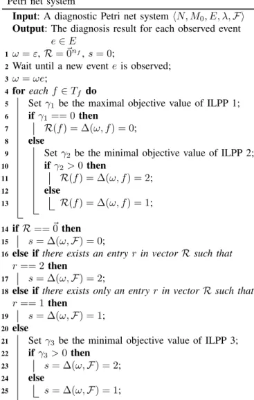
Algorithm 1: Online fault diagnosis using a diagnostic Petri net system
Input: A diagnostic Petri net system hN, M0, E, λ, F i
Output: The diagnosis result for each observed event e ∈ E
1 ω = ε, R = ~0nf, s = 0;
2 Wait until a new event e is observed;
3 ω = ωe;
4 for each f ∈ Tf do
5 Set γ1 be the maximal objective value of ILPP 1;
6 if γ1== 0 then
7 R(f ) = ∆(ω, f ) = 0;
8 else
9 Set γ2 be the minimal objective value of ILPP 2;
10 if γ2> 0 then 11 R(f ) = ∆(ω, f ) = 2; 12 else 13 R(f ) = ∆(ω, f ) = 1; 14 if R == ~0 then 15 s = ∆(ω, F ) = 0;
16 else if there exists an entry r in vector R such that
r == 2 then
17 s = ∆(ω, F ) = 2;
18 else if there exists only an entry r in vector R such that
r == 1 then
19 s = ∆(ω, F ) = 1;
20 else
21 Set γ3 be the minimal objective value of ILPP 3; 22 if γ3> 0 then
23 s = ∆(ω, F ) = 2;
24 else
25 s = ∆(ω, F ) = 1;
26 Output R and s and write them into log file; Goto 2;
14–19, we compute ∆(ω, F ) according to the diagnosis of each f ∈ Tf, i.e., R. If ∆(ω, F ) cannot be directly obtained by
R, we have to solve ILPP 3 to determine ∆(ω, F ) according to Corollary 3 (Lines 21–25). When the algorithm completes the diagnosis of the current step, it returns to Line 2 to wait for a new observed event.
The main computational cost of Algorithm1stems from the solutions of ILPPs 1, 2, 3. As known, solving an integer linear programming problem is NP-hard. Further, the computational cost mainly depends on its size,, i.e., the number of integer variables and constraints. We next analyze the size of the programming problem Eq. (2).
For ω = e1. . . eh, it is readily to verify that the number of
variables in Eq. (2) can be represented as
I = (nu+ ne1) + (nu+ ne2) + . . . + (nu+ neh)
= h · nu+ (ne1+ . . . + neh) ≈ h · (nu+ nf),
where nu= |Tu|1, nf = |Tf|, nei = |Tei|. Eq. (2) contains h
1| · | denotes the cardinality of a set.
groups of constraints and (nu+ nei) denotes the number of
variables in the ith group. Specifically, nu denotes the length
of vector yi and nei the number of binary variables, i.e.,
zei
1 , . . . , zneiei. At the same time, the number of constraints is
represented as
J = (m · ne1+ 1) + . . . + (m · neh+ 1)
= m · (ne1+ . . . + neh) + h ≈ h · (m · nf+ 1),
where m is the number of places in a labeled Petri net. For ei∈ ω, there are nei transitions whose labels are ei. Thus for
the ith group of constraints, it contains m·nei+1 constraints in
scalar form, where “1” denotes the constraint zei
1 +. . .+z ei
nei =
nei− 1.
In summary, the number of variables and constraints in Eq. (2) is linear in the length of the observed word. If the observed word is very long, we may not be able to obtain the diagnosis result in real time. However, the approach based on ILP is straightforward and easy to implement, and can be used as a basis to develop more efficient approaches.
TABLE II
DIAGNOSIS RESULT AND RUNNING TIME FOREXAMPLE2.
e1 e2 e3 e4 a b b a f1 0 1 1 1 f2 0 0 1 1 f3 0 0 0 0 F 0 1 2 2 Time (s) 0.0115 0.0107 0.0209 0.0233
Example 2. Let us consider the net shown in Fig.1. Assume that the observed word is ω = abba. The diagnosis result and running time are shown in Table II, where, for each event ei, there is a column which lists the diagnosis result and
running time corresponding to ei. For example, considering
e3 = b (i.e., ω = e1e2e3 = abb), the diagnosis results are
∆(ω, f1) = 1, ∆(ω, f2) = 1, ∆(ω, f3) = 0, and ∆(ω, F ) = 2
and the running time is 0.0209s. Note that the time is obtained by executing a MATLAB procedure with GUROBI solver (academic license) [33] on a laptop computer with Intel i5-4200M 2.5GHz processor and 8G DDR3 1600Hz RAM.
V. DIAGNOSABILITY AND OVERALL FAULT STATUS
The diagnosability of a Petri net is discussed in [34]–[36]. If a fault f is diagnosable, then the occurrence of f can be detected in a finite number of steps. Given a Petri net language L, its post-language after a transition sequence σ ∈ L
is defined as L/σ = {τ ∈ T∗ | στ ∈ L}. Formally, the
diagnosability of f is defined as follows.
Definition 4. [35] Given a labeled net hN, M0, E, λi, a fault
transition f is diagnosable if there exists an integer K ∈ N such that
∀σ = ˜σf ∈ L(N, M0), ∀τ ∈ L(N, M0)/σ with |τ | > K
If all fault transitions of a Petri net system are diagnosable, then the Petri net system is said to be diagnosable. For a diag-nosable labeled Petri net, we have the following proposition. Proposition 2. Consider a diagnosable labeled Petri net sys-tem hN, M0, E, λi with an overall fault status F . For each
sequence σf σ0 ∈ L(N, M0), it holds ∆(ω, F ) = 2, where
σ ∈ T∗, f ∈ Tf, σ0∈ T∗ with |σ0| > K, and ω = λ(σf σ0).
Proof. Since f is diagnosable, for each σ1∈
←−
C (ω), it holds f ∈ σ1. Thus, we have ∆(ω, F ) = 2 by Definition3.
In plain words, when a system is running, a fault f ∈ Tf
occurs and the process continues. After K steps, we are sure that f has occurred according to the observation ω. Thus, ∆(ω, f ) = 2 is true, which implies ∆(ω, F ) = 2.
Only when the Petri net model of a system is diagnosable (or I-diagnosable [1]), can the diagnosis algorithms detect unambiguously which faults have occurred. However, due to the use of overall fault status F , even if a net model of a system is not diagnosable, it is possible to detect the occurrence of faults in the system though we do not know exactly which fault occurs. An example is provided to clarify this. t1(a) p1 p2 p3 p4 t6(e) t8(c) f1 f2 t5(a) t4(b) t7(b) t3(b) p5 p6 p7 t2(c)
Fig. 4. A Petri net that is not diagnosable.
Example 3. Consider the net shown in Fig. 4, where Tu =
{t6, f1, f2} and Tf = {f1, f2}. According to Definition 4,
both f1and f2are not diagnosable. Assume that the observed
word is ω = (abb)(abb) · · · . Then it holds ∆(ω, f1) =
∆(ω, f2) = 1, i.e., the diagnosis results of f1 and f2 are
ambiguous for infinite ω. However, for ω0 = abb, it holds ∆(ω0, F ) = 2, i.e., when observing only abb, we have already known that some faults occur in the system. In this case, although we are sure that at least a fault has occurred, we are unable to exactly identify which faults have occurred. In real-world systems, a possible strategy is to stop the plant and inspect the faults one by one.
VI. CASE STUDY
We in this section explore the computational overhead of the proposed algorithm and compare its efficiency with the one shown in [30] by an example. Consider the labeled Petri net shown in Fig.5that is originally introduced in [20] and slightly modified in this paper, where Tu = {t1, f1, t4, t11, f2}, Tf =
{f1, f2}, Ta = {t3, t5, t6, t8}, Te = {t7, t9, t10, t12}, Th =
{t16}, Tg= {t14, t15, t17}. The initial marking is M0= p1+
αp2+ βp3, where α and β are two variables denoting the
numbers of tokens in p2 and p3, respectively.
a b t1 t4 t8(a) t12(e) t16(h) t5(a) t9(e) t17(g) t6(a) t10(e) t14(g) t3(a) t7(e) t11 t15(g) f1 f2 p1 p2 p3 p4 p5 p6 p7 p8 p9 p10 p11 p12 p13 p14 p15 p16
Fig. 5. A Petri net for case study.
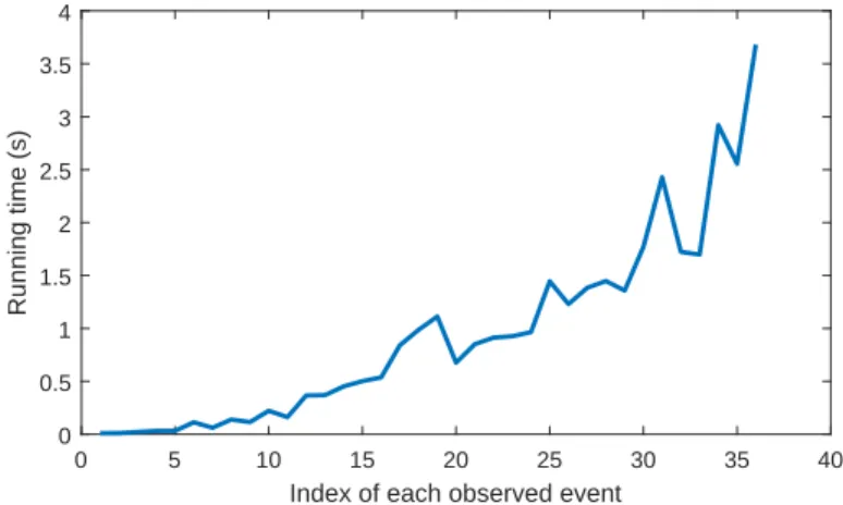
Let α = 10 and β = 10, and assume that the observed word is ω = ae(aeg)10gggg, where (aeg)10 represents that
the sequence aeg repeats 10 times. When observing an event, we make a diagnosis using Algorithm1. The running time of Algorithm1for each observed event is shown in Fig.6, where the x-axis represents the index of each event in sequence ω.
0 5 10 15 20 25 30 35 40
Index of each observed event 0 0.5 1 1.5 2 2.5 3 3.5 4 Running time (s)
Fig. 6. Running time for each observed event.
We have shown in SectionIVthat the size of programming model Eq. (2) is linear with respect to the length of the observed word. However, the difficulty of a generic ILP problem always increases exponentially with respect to its size, which is verified by Fig. 6. This implies that one probably cannot obtain the diagnosis result in real time if the observed sequence is very long. However, integer linear programming is a standard mathematical tool for diagnosis of Petri nets based on which some new approaches can be developed to overcome the complexity issue, which will be done in our subsequent work.
Fanti et al. [30] also proposed an algorithm for fault diag-nosis using labeled Petri nets and integer linear programming. However, the key idea is different from us. They first build an integer programming problem according to a transition sequence σ ∈ To∗ not an observed word ω ∈ E∗. Then, for
an observed word ω, they explore all possible sequences of observable transitions whose projections over E are equal to ω. The size of the programming problem in [30] is smaller
than the one in this paper. However, it has to be solved more times to obtain the diagnosis result.
The output and computational process of the algorithm proposed by Fanti et al. [30] are different from ours. In order to compare the efficiency of these two algorithms, we have to modify one of them to make them have the same input and output. We here choose to modify Fanti’s algorithm, though it is completely feasible to modify our algorithm (note that modifying our algorithm will lose some diagnostic informa-tion). The details of the modification of Fanti’s algorithm is discussed in Appendix A and this section mainly focuses on the comparison of these two algorithms. On the other hand, our algorithm, i.e., Algorithm 1, and the modified version of Fanti’s algorithm are both implemented in MATLAB language. The readers can refer to [37] for the source code.
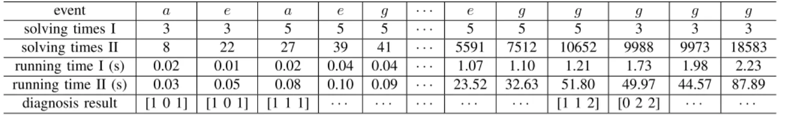
Consider the net in Fig.5again and assume that α = β = 7. If the observed word is ω = ae(aeg)7gggg, the comparison of these two algorithms is shown in TableIII. The first row lists all events in ω. The second row shows the number of times to solve the programming problems defined in this paper when performing diagnosis using the proposed algorithm. The third row shows the number of times to solve the programming problems defined in [30] when dealing with the diagnosis issue using the algorithm (modified version) developed in [30]. The fourth and fifth rows demonstrate the running time of diagnosis algorithms proposed by us and Fanti et al. [30], respectively. The running time is tested using GUROBI solver
[33] on a laptop computer with Intel i5-4200M 2.5GHz
processor and 8G DDR3 1600Hz RAM. The sixth row lists the diagnosis result for each event, which is represented as a row vector [a b c] such that ∆(ω, f1) = a, ∆(ω, f2) = b,
and ∆(ω, F ) = c. Note that the diagnosis of the fourth event from the last is [1 1 2], i.e., we detect the occurrence of faults (∆(ω, F ) = 2) before the exact faults are ascertained. The detailed comparison of running time is also illustrated by Fig.7. We observe that our approach is more efficient in this example.
0 5 10 15 20 25 30
Index of each observed event 0 20 40 60 80 100 Running time (s) Our approach
Approach proposed by Fanti et al.
Fig. 7. Comparison of our approach with the one in [30].
VII. CONCLUSION
This paper addresses the problem of fault diagnosis by formulating and solving ILP problems. The main contributions consist in introducing the overall fault status and proposing
an online diagnosis algorithm based on labeled Petri nets, in which two or more transitions can share the same label. The overall fault status provides a more informative diagnosis result, i.e., not only every fault but also the global system fault status can be detected. In addition, we show that, in some cases, a definite conclusion on the occurrence of faults in a system can be given even if the system is not diagnosable. We also compare the efficiency of the proposed approach with the one in [30] by a case study and the result shows that our approach is usually more efficient.
In future work, we plan to extend and modify the other diagnosis approaches, such as those in [25] and [21], to make them have a uniform interface. Then, we will develop a software package to compare their efficiency. On the other hand, we will explore the use of an overall fault status in a distributed environment.
REFERENCES
[1] M. Sampath, R. Sengupta, S. Lafortune, K. Sinnamohideen, and D. Teneketzis, “Diagnosability of discrete-event systems,” IEEE Trans-actions on Automatic Control, vol. 40, no. 9, pp. 1555–1575, 1995. [2] ——, “Failure diagnosis using discrete-event models,” IEEE
Transac-tions on Control Systems Technology, vol. 4, no. 2, pp. 105–124, 1996. [3] Y. F. Chen, Z. W. Li, K. Barkaoui, N. Q. Wu, and M. C. Zhou, “Compact supervisory control of discrete event systems by Petri nets with data inhibitor arcs,” IEEE Transactions on Systems, Man, and Cybernetics: Systems, vol. 47, no. 2, pp. 364–379, 2017.
[4] Y. F. Chen, Z. W. Li, K. Barkaoui, and A. Giua, “On the enforcement of a class of nonlinear constraints on Petri nets,” Automatica, vol. 55, pp. 116–124, 2015.
[5] G. H. Zhu, Z. W. Li, and N. Q. Wu, “Model-based fault identification of discrete event systems using partially observed Petri nets,” Automatica, vol. 96, pp. 201–212, 2018.
[6] A. Giua and C. Seatzu, “Identification of free-labeled Petri nets via integer programming,” in Proceedings of the 44th IEEE Conference on Decision and Control, Seville, Spain, 2005, pp. 7639–7644.
[7] Z. He, Z. W. Li, and A. Giua, “Performance optimization for timed weighted marked graphs under infinite server semantics,” IEEE Trans-actions on Automatic Control, vol. 63, no. 8, pp. 2573–2580, 2018. [8] W. M. P. van der Aalst, Process Discovery: An Introduction. New York,
NY, USA: Springer, 2011.
[9] H. M. Zhang, L. Feng, and Z. W. Li, “A learning-based synthesis approach to the supremal nonblocking supervisor of discrete-event systems,” IEEE Transactions on Automatic Control, vol. 63, no. 10, pp. 3345–3360, 2018.
[10] Z. Y. Ma, Y. Tong, Z. W. Li, and A. Giua, “Basis marking representation of Petri net reachability spaces and its application to the reachability problem,” IEEE Transactions on Automatic Control, vol. 62, no. 3, pp. 1078–1093, 2017.
[11] Y. Tong, Z. W. Li, C. Seatzu, and A. Giua, “Verification of state-based opacity using Petri nets,” IEEE Transactions on Automatic Control, vol. 62, no. 6, pp. 2823–2837, 2017.
[12] F. Basile, M. P. Cabasino, and C. Seatzu, “State estimation and fault di-agnosis of labeled time Petri net systems with unobservable transitions,” IEEE Transactions on Automatic Control, vol. 60, no. 4, pp. 997–1009, 2015.
[13] D. Lefebvre, “On-line fault diagnosis with partially observed Petri nets,” IEEE Transactions on Automatic Control, vol. 59, no. 7, pp. 1919–1924, 2014.
[14] L. Li and C. N. Hadjicostis, “Minimum initial marking estimation in labeled Petri nets,” IEEE Transactions on Automatic Control, vol. 58, no. 1, pp. 198–203, 2013.
[15] J. Prock, “A new technique for fault detection using Petri nets,” Auto-matica, vol. 27, no. 2, pp. 239–245, 1991.
[16] Y. Wu and C. N. Hadjicostis, “Algebraic approaches for fault iden-tification in discrete-event systems,” IEEE Transactions on Automatic Control, vol. 50, no. 12, pp. 2048–2055, 2005.
[17] A. Ram´ırez-Trevi˜no, E. Ruiz-Beltr´an, I. Rivera-Rangel, and E. Lopez-Mellado, “Online fault diagnosis of discrete event systems. A Petri net-based approach,” IEEE Transactions on Automation Science and Engineering, vol. 4, no. 1, pp. 31–39, 2007.
TABLE III
COMPARISON OF OUR APPROACH WITH THE ONE IN[30].
event a e a e g · · · e g g g g g solving times I 3 3 5 5 5 · · · 5 5 5 3 3 3 solving times II 8 22 27 39 41 · · · 5591 7512 10652 9988 9973 18583 running time I (s) 0.02 0.01 0.02 0.04 0.04 · · · 1.07 1.10 1.21 1.73 1.98 2.23 running time II (s) 0.03 0.05 0.08 0.10 0.09 · · · 23.52 32.63 51.80 49.97 44.57 87.89 diagnosis result [1 0 1] [1 0 1] [1 1 1] · · · [1 1 2] [0 2 2] · · · ·
[18] A. Benveniste, E. Fabre, S. Haar, and C. Jard, “Diagnosis of asyn-chronous discrete-event systems: a net unfolding approach,” IEEE Trans-actions on Automatic Control, vol. 48, no. 5, pp. 714–727, 2003. [19] J. Zaytoon and S. Lafortune, “Overview of fault diagnosis methods for
discrete event systems,” Annual Reviews in Control, vol. 37, no. 2, pp. 308–320, 2013.
[20] S. Genc and S. Lafortune, “Distributed diagnosis of discrete-event systems using Petri nets,” in Proceedings of International Conference on Application and Theory of Petri Nets, Eindhoven, the Netherlands, 2003, pp. 316–336.
[21] A. Giua and C. Seatzu, “Fault detection for discrete event systems using Petri nets with unobservable transitions,” in Proceedings of the 44th IEEE Conference on Decision and Contro, Seville, Spain, 2005, pp. 6323–6328.
[22] M. P. Cabasino, A. Giua, and C. Seatzu, “Fault detection for discrete event systems using Petri nets with unobservable transitions,” Automat-ica, vol. 46, no. 9, pp. 1531–1539, 2010.
[23] M. P. Cabasino, A. Giua, M. Pocci, and C. Seatzu, “Discrete event diagnosis using labeled Petri nets. An application to manufacturing systems,” Control Engineering Practice, vol. 19, no. 9, pp. 989–1001, 2011.
[24] M. P. Cabasino, A. Giua, A. Paoli, and C. Seatzu, “Decentralized diagnosis of discrete-event systems using labeled Petri nets,” IEEE Transactions on Systems, Man, and Cybernetics: Systems, vol. 43, no. 6, pp. 1477–1485, 2013.
[25] F. Basile, P. Chiacchio, and G. De Tommasi, “An efficient approach for online diagnosis of discrete event systems,” IEEE Transactions on Automatic Control, vol. 54, no. 4, pp. 748–759, 2009.
[26] M. Dotoli, M. P. Fanti, A. M. Mangini, and W. Ukovich, “On-line fault detection in discrete event systems by Petri nets and integer linear programming,” Automatica, vol. 45, no. 11, pp. 2665–2672, 2009. [27] Y. Ru and C. N. Hadjicostis, “Fault diagnosis in discrete event systems
modeled by partially observed Petri nets,” Discrete Event Dynamic Systems, vol. 19, no. 4, pp. 551–575, 2009.
[28] X. Wang, C. Mahulea, and M. Silva, “Diagnosis of time Petri nets using fault diagnosis graph,” IEEE Transactions on Automatic Control, vol. 60, no. 9, pp. 2321–2335, 2015.
[29] W. Hamscher, L. Console, and J. De Kleer, Readings in Model-Based Diagnosis. San Mateo, CA: Morgan Kaufmann, 1992.
[30] M. P. Fanti, A. M. Mangini, and W. Ukovich, “Fault detection by labeled Petri nets in centralized and distributed approaches,” IEEE Transactions on Automation Science and Engineering, vol. 10, no. 2, pp. 392–404, 2013.
[31] T. Murata, “Petri nets: Properties, analysis and applications,” Proceed-ings of the IEEE, vol. 77, no. 4, pp. 541–580, 1989.
[32] C. G. Cassandras and S. Lafortune, Introduction to discrete event systems. New York, NY, USA: Springer, 2009.
[33] Gurobi Optimizer. [Online]. Available:http://www.gurobi.com/
[34] M. P. Cabasino, A. Giua, and C. Seatzu, “Diagnosability of bounded petri nets,” in Proceedings of the 48th IEEE Conference on Decision and Control, Shanghai, China, 2009, pp. 1254–1260.
[35] ——, “Diagnosability of discrete-event systems using labeled Petri nets,” IEEE Transactions on Automation Science and Engineering, vol. 11, no. 1, pp. 144–153, 2014.
[36] F. Basile, P. Chiacchio, and G. De Tommasi, “On k-diagnosability of Petri nets via integer linear programming,” Automatica, vol. 48, no. 9, pp. 2047–2058, 2012.
[37] G. H. Zhu, “Matlab programs for this paper.” [Online]. Available:
https://github.com/zhuguanghui86/code for mypaper
APPENDIXA
MODIFICATION DETAILS OF THE ALGORITHM IN[30] The centralized fault diagnosis algorithm proposed in [30] has a different output with the one in this paper and thus we need to modify it, keeping the key idea unchanged, to compare its efficiency with our approach. We first briefly recall the ILP problem defined in [30] based on a sequence σo∈ To∗.
Given a sequence of observable transitions denoted by σo=
tα1tα2· · · tαh, the ILP problem without objective function can
be defined as M0+ Cu· i P k=1 yk+ i−1 P k=1 C(·, tαk) ≥ P re(·, tαi) yi∈ Nnu i = 1, . . . , h. (3)
By specifying different objective functions to Eq. (3), we obtain three ILP models:
ILPP 4: φ1= max h P i=1 yi(f ) s.t. Eq. (3) ILPP 5: φ2= min h P i=1 yi(f ) s.t. Eq. (3) ILPP 6: φ3= min ~11×nf· h P i=1 yi(Tf) s.t. Eq. (3).
On the basis of these ILP problems, the Fault Detection Algorithm (FDA) proposed in [30] (see Fig. 2 in [30]) is
modified as Algorithm 2 which takes a transition sequence
σo∈ To∗ as input. At the same time, the Diagnoser Algorithm
(DA) proposed in [30] (see Fig. 3 in [30]) is modified as
Algorithm 3 which enumerates all sequences of observable
transitions consistent with an observed word and repetitively calls Algorithm2. The data shown in rows 3 and 5 of TableIII
is computed by executing Algorithm3. The readers can inspect the souce code [37] for the details.
Note that the symbol ⊗ (not mentioned in [30]) in Line11
of Algorithm3is another contribution of this paper, which is a binary operation defined in Table IV and very appropriate to compute the combination of diagnosis results of transition sequences σo’s consistent with an observed word ω. We will
extend the approaches shown in [21] and [25] to the case of labeled Petri nets using this symbol in the subsequent research. We next show the formal definition of symbol ⊗ and prove its correctness.
Analogous to the labeling function λ, we define a new function τ : T → To∪ {ε} such that τ (t) = t if t ∈ To and
τ (t) = ε if t ∈ Tu. The function τ is extended to a sequence
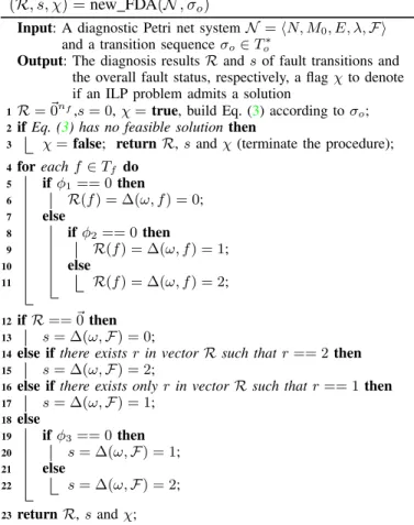
Algorithm 2: A fault diagnosis algorithm denoted by (R, s, χ) = new FDA(N , σo)
Input: A diagnostic Petri net system N = hN, M0, E, λ, F i
and a transition sequence σo∈ To∗
Output: The diagnosis results R and s of fault transitions and the overall fault status, respectively, a flag χ to denote if an ILP problem admits a solution
1R = ~0nf,s = 0, χ = true, build Eq. (3) according to σo; 2if Eq. (3) has no feasible solutionthen
3 χ = false; return R, s and χ (terminate the procedure); 4for each f ∈ Tf do 5 if φ1== 0 then 6 R(f ) = ∆(ω, f ) = 0; 7 else 8 if φ2== 0 then 9 R(f ) = ∆(ω, f ) = 1; 10 else 11 R(f ) = ∆(ω, f ) = 2; 12if R == ~0 then 13 s = ∆(ω, F ) = 0;
14else if there exists r in vector R such that r == 2 then 15 s = ∆(ω, F ) = 2;
16else if there exists only r in vector R such that r == 1 then 17 s = ∆(ω, F ) = 1; 18else 19 if φ3== 0 then 20 s = ∆(ω, F ) = 1; 21 else 22 s = ∆(ω, F ) = 2; 23return R, s and χ;
Algorithm 3: An online fault diagnosis algorithm Input: A diagnostic Petri net system N = hN, M0, E, λ, F i
Output: The diagnosis results R and s for each event e
1R = ~0nf, s = 0, Λ0= {ε}, α = true (α denotes if e is the
first event);
2Wait until a new event e is observed; Λ = ∅; 3for each t ∈ Te do 4 for each σ0o∈ Λ0 do 5 σo= σ0ot; (R 0 , s0, χ) = new FDA(N , σo); 6 if χ is true then 7 Λ = Λ ∪ {σo}; 8 if α is true then 9 R = R0, s = s0, α = false; 10 else 11 R = R ⊗ R0; s = s ⊗ s0; 12Λ0= Λ; 13Output R, s; Goto2;
the projection of σ ∈ T∗ on the set of observable transitions. For an observed word ω ∈ LE(N, M0), we denote
T (ω) = {ν ∈ T∗ o | σ ∈
←−
C (ω), ν = τ (σ)}
the set of observable projections of transition sequences con-sistent with ω.
Proposition 3. Given a diagnostic net system
hN, M0, E, λ, F i and an observed word ω ∈ E∗, for
TABLE IV BINARY OPERATION⊗. ⊗ 0 1 2 0 0 1 1 1 1 1 1 2 1 1 2 each f ∈ Tf ∪ {F }, it holds ∆(ω, f ) = ∆(ν1, f ) ⊗ ∆(ν2, f ) ⊗ . . . ⊗ ∆(νk, f ), (4) where k = |T (ω)|, {ν1, . . . , νk} = T (ω), and ⊗ : {0, 1, 2} ×
{0, 1, 2} → {0, 1, 2} is a binary operation defined in TableIV.
Proof. For f ∈ Tf ∪ {F } and ν ∈ T (ω), we can compute
∆(ν, f ) according to Algorithm2. T (ω) denotes all sequences of observable transitions whose projections on E are ω. Assume that there are only two items ν1 and ν2 in T (ω).
For f ∈ Tf, if ∆1 = ∆(ν1, f ) = 0 and ∆2= ∆(ν2, f ) = 0,
there is no fault f to occur in paths consistent with ν1and ν2
according to Definition 2, and thus we have ∆(ω, f ) = 0.
On the other hand, if ∆1 = 0 and ∆2 = 2, there is no
fault f in paths consistent with ν1 but fault f must occur
in all paths consistent with ν2. Thus, ∆(ω, f ) = 1 is true
according to Definition 2. Following a similar procedure, we obtain TableIVfor each f ∈ Tf∪{F } according to Definitions
2and3. If T (ω) contains more than two elements, Eq. (4) is readily verified.
![Fig. 7. Comparison of our approach with the one in [30].](https://thumb-eu.123doks.com/thumbv2/123doknet/14623368.733969/11.918.76.449.766.980/fig-comparison-approach.webp)