TCP Variants and Transfer Time Predictability in Very High Speed Networks

(1)

HAL Id: inria-00165781

https://hal.inria.fr/inria-00165781v2

Submitted on 30 Jul 2007

HAL is a multi-disciplinary open access

archive for the deposit and dissemination of sci-entific research documents, whether they are pub-lished or not. The documents may come from teaching and research institutions in France or abroad, or from public or private research centers.

L’archive ouverte pluridisciplinaire HAL, est destinée au dépôt et à la diffusion de documents scientifiques de niveau recherche, publiés ou non, émanant des établissements d’enseignement et de recherche français ou étrangers, des laboratoires publics ou privés.

High Speed Networks

Romaric Guillier, Sébastien Soudan, Pascale Vicat-Blanc Primet

To cite this version:

Romaric Guillier, Sébastien Soudan, Pascale Vicat-Blanc Primet. TCP Variants and Transfer Time Predictability in Very High Speed Networks. [Research Report] RR-6256, INRIA. 2007, pp.29. �inria-00165781v2�

(2)

a p p o r t

d e r e c h e r c h e

0 2 4 9 -6 3 9 9 IS R N IN R IA /R R --6 2 5 6 --F R + E N G Thème NUM

TCP Variants and Transfer Time Predictability in

Very High Speed Networks

Romaric Guillier — Sébastien Soudan — Pascale Vicat-Blanc Primet

N° 6256

(3)

(4)

Unité de recherche INRIA Rhône-Alpes

655, avenue de l’Europe, 38334 Montbonnot Saint Ismier (France)

Networks

Romaric Guillier, Sébastien Soudan, Pascale Vicat-Blanc Primet

Thème NUM — Systèmes numériques Projet RESO

Rapport de recherche n° 6256 — July 2007 — 26 pages

Abstract: In high performance distributed computing applications, data movements have demanding

performance requirements such as reliable and predictable delivery. Predicting the throughput of large transfers is very difficult in paths that are heavily loaded with just a few big flows. This report explores how current high speed transport protocols behave and may improve transfer time predictability of gigabits of data among endpoints in a range of conditions. In a fully controlled long distance 10 Gbps network testbed, we compare several TCP variants behaviour in presence of diverse congestion level and reverse traffic situations. We show that these factors have a very strong impact on transfer time predictability of several transport protocols.

Key-words: bulk data transfers, bandwidth sharing, transfer delay predictability, transport protocol

experimentation

This text is also available as a research report of the Laboratoire de l’Informatique du Parallélisme

(5)

Réseaux Trés Haut Débit

Résumé : Dans les applications hautes performances de calcul distribué, les mouvements de données

doivent fournir des garanties de performances, comme de la distribution fiable et prévisible. Prévoir le débit de larges transferts est difficile sur les chemins réseaux qui sont lourdement chargés par quelques gros flux. Ce rapport explore la façon dont les protocoles de transport haut débit se comportent et peuvent améliorer la prédictabilité des temps de transferts de gigaoctets de données entre des noeuds d’extrémité dans un éventail de conditions. Dans un environment de test complètement controlé avec un réseau longue distance à 10 Gbps, nous comparons le comportement de plusieurs variantes de TCP en présence de diffeérents niveaux de congestion et trafic sur le chemin retour. Nous montrons que ces facteurs ont un impact très important sur la prédictabilité du temps de transfert pour plusieurs protocoles de transport.

Mots-clés : partage de bande passante, expérimentation de protocole de transport, prédiction de temps de transfert total, transferts en masse de données

(6)

1 Introduction

In high performance distributed computing, like experimental analysis of high-energy physics, cli-mate modelling, and astronomy, massive datasets must be shared among different sites, and trans-ferred across network for processing. The movement of data in these applications have demanding performance requirements such as reliable and predictable delivery [FFR+04].

Generally, both distributed applications and high level communication libraries available on end systems use the socket API and TCP as transport protocol. TCP is a fully distributed congestion control protocol which statistically share available bandwidth among flows “fairly”. In Internet, where the endpoints’ access rates are generally much smaller (2 Mbps for DSL lines) than the backbone link’s capacity (2.5 Gbps for an OC48 link) these approaches used to be very efficient. It has also been shown that in such conditions, and particularly when the load is not too high and the degree of multiplexing in the bottleneck link is high, formula-based and history-based TCP throughput predictors give correct predictions [HDA05]. However for high-end applications, the bandwidth demand of a single endpoint (e.g.1 Gbps) is comparable to the capacity of bottleneck link. In such a low multiplexing environment, high congestion level may be not rare and a transient burst of load on the forward or on the reverse path may cause active transfers to miss their deadlines. For example, this situation might occur when processes belonging to different applications are exchanging input and output files simultaneously.

The goal of this report is then to explore this issue and to examine how recent transport pro-tocol enhancements could benefit to high-end applications in terms of data transfer efficiency and predictability in the absence of any access control and reservation mechanisms. It is centred on elephant-like bulk data transfers in very high-capacity (1 Gbps, 10 Gbps) networks these environ-ments are supposed to benefit today and on new TCP variant protocols that are currently available on end nodes. The systematic evaluation of the protocols in a fully controlled and real testbed called Grid’5000 provides a set of measurements of transfer time in a broad range of conditions. We explore mainly three factors: synchronisation of start time, congestion level and reverse traffic.

The report is organised as follows. In section 2, several protocols enhancements proposed are briefly surveyed. Section 3 describes our experimental methodology and testbed. Experimental results are given and analysed in section 4. We study systematically three factors influencing the protocol behaviour and affecting the predictability of data transfers. Related works are reviewed in section 5. Finally, we conclude in section 6 and propose some perspectives for protocol and network service enhancement.

2 Transport protocol variants and their characterisation

The enhancement of TCP/IP has been intensively pursued to tackle limits encounter in large bandwidth-delay product environment [WHVBPa05]. Different TCP variants have been proposed to improve the response function of AIMD congestion control algorithm in large bandwidth delay product networks. All these protocols are not equivalent and behave differently according the network and traffic con-ditions. In this report we concentrate on the TCP variants available in all recent GNU/Linux kernel: High Speed TCP, Scalable TCP, Hamilton-TCP, BIC-TCP and CUBIC.

To analyse the acquired data, several metrics can be used to synthetically characterise the be-haviour of different TCP variants [TMR07]. These metrics are: fairness, throughput, delay, goodput distribution, variance of goodput, utilisation, efficiency, transfer time. This paper is focused on the transfer time metric which can be considered as a throughput metric. Indeed, throughput can be mea-sured as a router-based metric of aggregate link utilisation, as a flow-based metric of per-connection

(8)

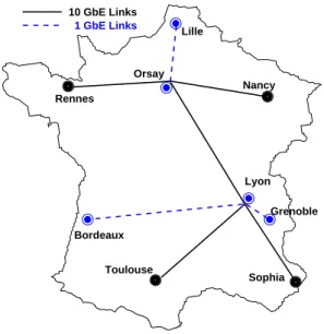
Nancy Grenoble Rennes Lille Sophia Toulouse 10 GbE Links Orsay Bordeaux 1 GbE Links Lyon

Figure 1: Grid’5000 backbone

transfer times, and as user-based metrics of utility functions or user waiting times. Throughput is distinguished from goodput, where throughput is the link utilisation or flow rate in bytes per sec-ond, and goodput, also measured in bytes per secsec-ond, is the subset of throughput consisting of useful traffic. We note that maximising throughput is of concern in a wide range of environments, from highly-congested to under-utilised networks, and from long-lived to very short flows. As an example, throughput has been evaluated in terms of the transfer times for connections with a range of transfer sizes for evaluating Quick-Start, a proposal to allow flows to start-up faster than slow start [SAF06].

3 Methodology

This report is associated with the Grid’5000 project, an experimental grid platform gathering 2500 processors over nine geographically distributed sites in France. It allows dynamic deployment of network stacks. The network infrastructure (see Figure 1) is an interconnection of LANs (i.e. grid sites) and an 10 Gbps lambda-based private network [BCC+_{06]. We are using iperf, GNU/Linux}

kernel version 2.6.16 with Web100 patch and CUBIC patch to perform our experiments.

Figure 2 presents the topology used in our experiments. It is a classical dumbbell, with N pairs of nodes able to send at 1 Gbps on each side. One flow by nodes’ pair is used to perform a file transfer. N is subdivided into two parts, according to the function assigned to the nodes. Nf refers to the number

of flows on the forward path (A → B) and Nrthe number of flows on the reverse path (B → A). The

bottleneck is the L2 switch. Here the Grid’5000 backbone could be the 10 Gbps link between Rennes and Toulouse (experiments at 19.8 ms RTT) or a 1 Gbps link between Rennes and Lyon (experiments at 12.8 ms RTT).

The congestion factor is defined as the ratio between the Nf nodes’ nominal capacity and the

bottleneck capacity. Similarly the reverse traffic factor is the ratio between the Nr nodes’ nominal

capacity and the bottleneck capacity. The multiplexing level is equal to Nf.

We explore starting time, congestion level and reverse traffic level parameters. We are considering several metrics, along with those defined in [GHK+07]. The primary metrics that will be used is the

(9)

Grid5000 backbone Side A Switch Switch 1Gbps 1Gbps PC PC Side B

Figure 2: Experiment topology

mean completion time, defined as: T = 1

Nf

PNf

i=1Ti where Ti is the completion time of the ith Nf

file transfer (typically, with sizes of 30 GB).

Additionally, we also use the following metrics:

Max completion time: Tmax= max(Ti)

Min completion time: Tmin = min(Ti)

Standard deviation of completion time σT = q

1 Nf orward

PNf orward

n=1 (Ti− T )2

Completion time coefficient of variation CoV = σT T

that are more suited than just mean values to characterise the variability of completion time. Each experiments for a given value of Nf, Nror protocols were executed at least three times to

ensure that our measures were consistent. By choice of the volume to transfer, an experiment would last an average of 400 s. The full experiment set for this report amount to more than 100 hours of experiments, which shows that doing real experiments is very time consuming. Also the logs we captured are amounting to more than 1.5 GB, even though we didn’t take precise Web100 logs for every experiments.

4 Results

In this section, we present the experiments that were made using a 10 Gbps bottleneck in Grid’5000. They were all performed between the Toulouse’s cluster (Sun Fire V20z) and Rennes’ cluster Parasol (Sun Fire V20z). The bottleneck is the access link of both sites. It is the output port of a 6500 Cisco in the Toulouse’s cluster and a 6509 Cisco in the Rennes’cluster Parasol.

4.1 Influence of starting time

The interval between each flow’s start is of importance as losses during slow start lead to ssthreshold moderation and may limit the achievable throughput during the whole transfer. Figure 3 illustrates the worst case: starting all flows simultaneously (within the same second) has the worst impact on the completion time of the flows and the best case: starting every flow outside the slow start phase of the

(10)

0 200 400 600 800 1000 1200 0 100 200 300 400 500 600 Goodput (Mbps) T (s) 17 Individual bic flows

(a) All flows starting at second 0

0 200 400 600 800 1000 1200 0 100 200 300 400 500 600 Goodput (Mbps) T (s) 17 Individual bic flows

(b) Each flow starts with a 4 s delay

(11)

TCP variant aX b Correlation Determination coefficient (r) coefficient (R2) Reno 267.68 0.090 0.993037 0.98612 BIC 217.96 85.97 0.984242 0.968732 Cubic 242.36 34.39 0.999619 0.999239 Highspeed 251.35 25.87 0.999134 0.99827 H-TCP 244.31 43.24 0.9989 0.9978 Scalable 182.45 136.21 0.977145 0.954812

Table 1: Linear regression for mean transfer time as a function of the congestion level without reverse traffic

others. The upper Figure 3(a) exhibits a set of flows experiencing drops during their slow start phase. These were unable to obtain a correct share during the rest of the experiment. Other grabbed a large portion of the bandwidth and completed in a short time (300 s). Even though the mean completion time in the worst case is better in Figure 3(b) (409 s vs 425 s), it has a much larger standard deviation (83 vs 28) than in the best case. We note that this parameter is especially important for the less aggressive TCP variants as they require a longer time to recover from these losses.

For the rest of our experiments, we choose to set the starting delay between transfers to 1 s to avoid potential harm from this parameter as in the best case, slow start takes in the best case(log2N − 1) ∗ RT T , for a congestion window of N packets [Jac88]. For a 19.7 ms RTT, N ≃1600 and slow start

lasts about 200 ms.

4.2 Congestion level

In this section, we are considering the impact of the congestion level factor alone on different TCP variants.

4.2.1 General Behaviour

Figure 4 shows the impact of high congestion level on every TCP variants. For example, we observe that the predictability of a transfer time with Scalable is bad as there is more than 300 s between the first and the last completion time. Even though each protocol is able to completely fill the link, they all have a different behaviour. The bandwidth sharing with Reno, BIC, CUBIC, Highspeed and H-TCP is fair among the various transfers leading to a smaller variance in the completion time.

4.2.2 Modelling

Table 1 presents the coefficients obtained through a linear regression of the mean transfer time for ev-ery TCP variant tested without reverse traffic. The models are only valid for congestion levels above or equal to 1.0. The linear model seems to fit fairly for most of the TCP variants for the range of congestion level studied (determination coefficient above 0.99). The only exception is Scalable for which the following model: 130.4∗X2

− 234.83 ∗ X + 454.83 seems to be more suited (determination

coefficient = 0.996432). These models are used in Figure 5 that presents the impact of the conges-tion level on mean compleconges-tion time for several TCP. The ideal TCP represented on the same figure corresponds to a TCP able to send continuously over 1 Gbps links, without slow start phase, without

(12)

0 200 400 600 800 1000 1200 0 100 200 300 400 500 600 700 Goodput (Mbps) T (s) 21 Individual reno flows

(a) Reno 0 200 400 600 800 1000 1200 0 100 200 300 400 500 600 700 Goodput (Mbps) T (s) 21 Individual bic flows

(b) BIC 0 200 400 600 800 1000 1200 0 100 200 300 400 500 600 700 Goodput (Mbps) T (s) 21 Individual cubic flows

(c) CUBIC 0 200 400 600 800 1000 1200 0 100 200 300 400 500 600 700 Goodput (Mbps) T (s) 21 Individual highspeed flows

(d) Highspeed 0 200 400 600 800 1000 1200 0 100 200 300 400 500 600 700 Goodput (Mbps) T (s) 21 Individual htcp flows (e) H-TCP 0 200 400 600 800 1000 1200 0 100 200 300 400 500 600 700 Goodput (Mbps) T (s) 21 Individual scalable flows

(f) Scalable

Figure 4: Impact of a high congestion level: 2.1 congestion level (21 flows), 19.8 ms RTT, on CUBIC and Scalable

(13)

200 250 300 350 400 450 500 550 600 0.7 0.9 1.1 1.3 1.5 1.7 1.9 2.1

Mean completion time

Congestion level Ideal TCP Reno no reverse Bic no reverse Cubic no reverse Highspeed no reverse Htcp no reverse Scalable no reverse

Figure 5: Impact of congestion level on the mean completion time for all TCP variants

losses or retransmissions and with equal sharing of the bottleneck link. All protocols, except Scalable, behave similarly: Our previous work [GHK+07] has shown that for the RTT used in our experiments here, most TCP variants tend to have similar performance.

We can see that the models are continuous but not differentiable when congestion appears. The completion time of transfers is nearly constant when there is no congestion. Scalable is displaying an asymptotic behaviour. The fact that the slopes for CUBIC and the ideal TCP are very close (242 to 252) might indicate that for a greater number of transfers we may observe an asymptotic behaviour too. It may be linked to aspects of Altman’s modelling of TCP Reno using parallel transfers [ABTV06].

4.2.3 Predictability

Figure 6 presents the completion time distribution of all the TCP variants. Scalable is somewhat remarkable as it is often displaying the shortest and the longest completion time for a given Nf. Even

though both distributions are roughly Gaussian-shaped, Scalable is more spreaded out (294 s vs 114 s for the 2.1 congestion level case) than CUBIC for instance. It makes Scalable a poor choice if we need to wait for all transfers to complete. But if we can start computation on a limited dataset (like a DNA sequencing), we might be able to increase the usage of the computation nodes. It might not be the case in other applications like astronomy interferometry that will need full transfer of all images before the start of a computation phase. It seems that HighSpeed TCP is the best choice if we are interested in good predictability, as it has the lowest dispersion of all protocols for high congestion levels.

Figure 7 presents the evolution of the completion time CoV for all the TCP variants tested. Here we can see that they all display the same kind of tendency as they all seem to be following a parabola as the congestion level increases. The apex of the parabola seems to depend on the protocol. This behaviour might indicate that there is a congestion level/multiplexing level region in which we should not be so as to minimise the variability of our completion time (and thus increase the predictability)

(14)

200 400 600 800 0.9 1.1 1.3 1.5 1.7 1.9 2.1 0 0.1 0.2 0.3 0.4 Congestion factor Completion time (s) Density Reno (a) Reno 200 400 600 800 0.9 1.1 1.3 1.5 1.7 1.9 2.1 0 0.1 0.2 0.3 0.4 Congestion factor Completion time (s) Density Bic (b) BIC 200 400 600 800 0.9 1.1 1.3 1.5 1.7 1.9 2.1 0 0.1 0.2 0.3 0.4 0.5 Congestion factor Completion time (s) Density CUBIC (c) CUBIC 200 400 600 800 0.9 1.1 1.3 1.5 1.7 1.9 2.1 0 0.1 0.2 0.3 0.4 Congestion factor Completion time (s) Density Highspeed (d) HighSpeed 200 400 600 800 0.9 1.1 1.3 1.5 1.7 1.9 2.1 0 0.1 0.2 0.3 0.4 0.5 Congestion factor Completion time (s) Density Htcp (e) H-TCP 200 400 600 800 0.9 1.1 1.3 1.5 1.7 1.9 2.1 0 0.1 0.2 0.3 0.4 Congestion factor Completion time (s) Density Scalable (f) Scalable

(15)

0 0.02 0.04 0.06 0.08 0.1 0.12 0.14 0.7 0.9 1.1 1.3 1.5 1.7 1.9 2.1

Completion time coefficient of variation

Congestion level Reno no reverse Bic no reverse Cubic no reverse Highspeed no reverse Htcp no reverse Scalable no reverse

Figure 7: Evolution of the completion time coefficient of variation as a function of the congestion level for several TCP variants

We can also note that most TCP variants’ CoV stays below 6 %. This means that if we are not able to control the way transfers are started to ensure that we are well under the congestion level, we would have to consider at least a 6 % margin on an estimated completion time to be sure not to fail the deadline in the case when there is no reverse traffic. If we assume that the distribution of the completion time is indeed Gaussian, using such a margin would provide a 68 % confidence interval for the completion of our transfers. If we want a more precise (say 95 % confidence interval), we would need to push the margin up to 12 %. But adding such a big margin is not the best solution, especially if the transfers have very strict windows and if we want to be efficient.

(16)

5000 6000 7000 8000 9000 10000 0 100 200 300 400 500 Aggregate goodput (Mbps) T (s) Reno 90% reverse traffic Reno 110% reverse traffic

(a) Reno 5000 6000 7000 8000 9000 10000 0 100 200 300 400 500 Aggregate goodput (Mbps) T (s) Bic 90% reverse traffic Bic 110% reverse traffic

(b) BIC 5000 6000 7000 8000 9000 10000 0 100 200 300 400 500 Aggregate goodput (Mbps) T (s) Cubic 90% reverse traffic Cubic 110% reverse traffic

(c) CUBIC 5000 6000 7000 8000 9000 10000 0 100 200 300 400 500 Aggregate goodput (Mbps) T (s) Highspeed 90% reverse traffic Highspeed 110% reverse traffic

(d) Highspeed 5000 6000 7000 8000 9000 10000 0 100 200 300 400 500 Aggregate goodput (Mbps) T (s) Htcp 90% reverse traffic Htcp 110% reverse traffic (e) H-TCP 5000 6000 7000 8000 9000 10000 0 100 200 300 400 500 Aggregate goodput (Mbps) T (s) Scalable 90% reverse traffic Scalable 110% reverse traffic

(f) Scalable

Figure 8: Comparison of aggregate goodput for 1.8 congestion level according to the level of reverse traffic

4.3 Reverse traffic impact

The reverse traffic here consists in similar large 30 GB file transfers as in the forward path. The reverse transfers are started after the forward transfers with the same interval of 1 s to prevent interactions during the slow start phase just as stated in Section 4.1. We are only considering what is happening on the transfer time for the forward path when there is reverse traffic.

(17)

0 200 400 600 800 1000 1200 1400 1600 0 100 200 300 400 500 600 0 1000

Individual goodput (Mbps) _{Aggregated goodput (Mbps)}

T (s) Flow 1 Cubic

Flow 2 Cubic cubic Sum

(a) no reverse traffic

0 200 400 600 800 1000 1200 1400 1600 0 100 200 300 400 500 600 700 800 900 0 1000

T (s) Flow 1 Cubic

Flow 2 Cubic cubic Sum

(b) 2.0 reverse traffic level (2 flows)

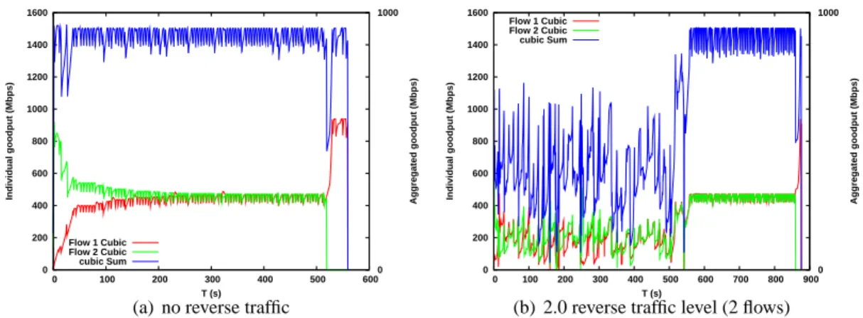
Figure 9: Impact of reverse traffic: CUBIC, 2.0 congestion level (2 flows), 12.8 ms RTT

4.3.1 General behaviour

In Figure 8, we compare the impact of a non-congesting (0.9) and a congesting (1.1) reverse traffic level for a given congestion level (1.8) on the aggregate goodput of all the participating transfers. Here again, we can observe that most protocols present a very similar pattern. For the non-congesting case, they all present some sort of hollow during the period in which the transfers on the reverse path are active that is likely to be caused by the bandwidth taken by the ACKs from the reverse traffic (about 200 Mbps). H-TCP and Reno are the only protocols whose aggregate goodput displays some instabilities. The other are mostly stable during the period.

For the congesting case, we can see that the aggregate goodput is not stable at all for most protocols and we can observe aggregate goodput drops of more than 2 Gbps that last for more than a few seconds for some protocols like CUBIC. It seems to be due to synchronises losses on the forward path. This indicates that we are clearly not efficient and that have congesting reverse traffic might lead to miss deadlines if it is not taken into account. Scalable is the protocol that seems to be the least impacted by this phenomena as the amplitude of the aggregate goodput spikes are less than 1 Gbps.

4.3.2 Multiplexing factor

In Figure 9, we observe that reverse traffic has a huge impact, as aggregated goodput is nearly halved during reverse traffic presence and the latest completion time goes from 562 s to 875 s. In this exper-iment, only a small number of flows (2) were used as the bottleneck size is 1 Gbps.

In the following experiment, as shown on Figure 10, the bottleneck size is 10 Gbps and we were using ten times more flows than in the previous setting. In this configuration, we observe that the mul-tiplexing level (or number of nodes emitting simultaneously) is an important parameter as for similar congestion and reverse traffic level using a more important number of nodes yield better results: about 617 s (30 % faster). Even though, we observe that the aggregate goodput is also deeply affected in Figure 10, its variation only amounts up to 20 % of the available bandwidth. In the Figure 9, the variation is more like 50 % of the available bandwidth.

4.3.3 Modelling

In this section, we try provide models for the TCP variants’ mean completion time as a function of the congestion level under reverse traffic. They are given in Table 2, 3, 4 and 5. Linear models seem

(18)

0 200 400 600 800 1000 1200 1400 1600 0 100 200 300 400 500 600 700 0 1000 2000 3000 4000 5000 6000 7000 8000 9000 10000

T (s) cubic Sum

(a) no reverse traffic

0 200 400 600 800 1000 1200 1400 1600 0 100 200 300 400 500 600 700 0 1000 2000 3000 4000 5000 6000 7000 8000 9000 10000

T (s) cubic Sum

(b) 2.0 reverse traffic level (20 flows)

Figure 10: Impact of reverse traffic: CUBIC, 2.0 congestion level (20 flows), 19.8 ms RTT

Table 2: Linear regression for mean transfer time as a function of the congestion level with 0.7 reverse traffic level (7 flows)

to fit rather well (determination coefficient above 0.98). The only exception is again Scalable, like in Table 1, for which a linear model doesn’t fit well (determination coefficients varying between 0.87 and 0.96). Using regression with an higher polynomial degree doesn’t see to improve much the accuracy of the model. It could mean that the variability already noticed of Scalable is too important and that 3 instances of a given test weren’t just enough to capture a good modelling of it.

The slopes for 0.7, 1.1 and no reverse traffic level are very similar to each other for most protocols. It indicates that reverse traffic’s impact could be seen as a reduction of the available bandwidth.

Figure 11, 12, 13, 14, 15 and 16 present the effect of different levels of reverse traffic on the mean completion time for every protocol.

For instance for CUBIC (Figure 13, we can see that for reverse traffic level lower than 1.0, its effect is limited on the mean completion time (about 2.5 %). The fluctuations observed for 0.9 reverse traffic level are mainly due to the fact that we are close to the congestion gap and thus to a very instable point. When the reverse traffic is congesting, we observe that the difference with the case without reverse traffic is much more important (about 10 %).

Some other results are also very interesting, such as the fact that for BIC in Figure 12 adding a little dose of reverse traffic (i.e. non-congesting) seems to be interesting as it appears to be more efficient in these conditions, especially if the congesting level is high. Similar behaviours may be seen in other protocols, for H-TCP (Figure 15) and for Highspeed (Figure 14), but it only seems to occur for very large value of congestion level.

(19)

TCP variant aX b Correlation Determination coefficient (r) coefficient (R2) Reno 304.88 -12.34 0.993149 0.986344 BIC 280.5 24.66 0.999728 0.999456 Cubic 268.7 35.93 0.998006 0.996016 Highspeed 310.52 -18.49 0.996203 0.99242 H-TCP 275.84 60.05 0.998776 0.997553 Scalable 203.75 131.078 0.969326 0.939592

Table 5: Linear regression for mean transfer time as a function of the congestion level with symetric reverse traffic level

(20)

200 250 300 350 400 450 500 550 600 0.7 0.9 1.1 1.3 1.5 1.7 1.9 2.1

Congestion level Reno no reverse Reno 0.7 reverse traffic level Reno 0.9 reverse traffic level Reno 1.1 reverse traffic level Reno symetric reverse

Figure 11: Impact of the reverse traffic on the mean completion time for Reno, 19.8 ms RTT

200 250 300 350 400 450 500 550 600 0.7 0.9 1.1 1.3 1.5 1.7 1.9 2.1

Congestion level Bic no reverse

Bic 0.7 reverse traffic level Bic 0.9 reverse traffic level Bic 1.1 reverse traffic level Bic symetric reverse

(21)

200 250 300 350 400 450 500 550 600 0.7 0.9 1.1 1.3 1.5 1.7 1.9 2.1

Congestion level Cubic no reverse Cubic 0.7 reverse traffic level Cubic 0.9 reverse traffic level Cubic 1.1 reverse traffic level Cubic symetric reverse

Figure 13: Impact of reverse traffic level on mean completion time for CUBIC, 19.8 ms RTT

200 250 300 350 400 450 500 550 600 0.7 0.9 1.1 1.3 1.5 1.7 1.9 2.1

Congestion level Highspeed no reverse Highspeed 0.7 reverse traffic level Highspeed 0.9 reverse traffic level Highspeed 1.1 reverse traffic level Highspeed symetric reverse

(22)

200 250 300 350 400 450 500 550 600 0.7 0.9 1.1 1.3 1.5 1.7 1.9 2.1

Congestion level Htcp no reverse Htcp 0.7 reverse traffic level Htcp 0.9 reverse traffic level Htcp 1.1 reverse traffic level Htcp symetric reverse

Figure 15: Impact of the reverse traffic on the mean completion time for H-TCP, 19.8 ms RTT

200 250 300 350 400 450 500 550 600 0.7 0.9 1.1 1.3 1.5 1.7 1.9 2.1

Congestion level Scalable no reverse Scalable 0.7 reverse traffic level Scalable 0.9 reverse traffic level Scalable 1.1 reverse traffic level Scalable Symetric reverse

(23)

0 200 400 600 800 1000 1200 1400 1600 0 50 100 150 200 250 300 350 400 450 0 1000 2000 3000 4000 5000 6000 7000 8000 9000 10000 Goodput (Mbps) T (s) cubic Sum (a) No reverse 0 200 400 600 800 1000 1200 1400 1600 0 50 100 150 200 250 300 350 400 450 0 1000 2000 3000 4000 5000 6000 7000 8000 9000 10000 Goodput (Mbps) T (s) cubic Sum (b) 0.9 reverse 0 200 400 600 800 1000 1200 1400 1600 0 50 100 150 200 250 300 350 400 450 500 0 1000 2000 3000 4000 5000 6000 7000 8000 9000 10000 Goodput (Mbps) T (s) cubic Sum (c) 1.1 reverse 0 200 400 600 800 1000 1200 1400 1600 0 50 100 150 200 250 300 350 400 450 500 0 1000 2000 3000 4000 5000 6000 7000 8000 9000 10000 Goodput (Mbps) T (s) cubic Sum (d) 1.5 reverse

Figure 17: Effect of various reverse traffic level on a fixed congestion level for CUBIC, 19.8 ms RTT

All in all, we can see that the protocols are reacting to the fact that the reverse traffic is congesting or not as it can be seen on Figure 17 for CUBIC. There we can see that once the reverse traffic is congesting, there is little more effect on the protocol behaviour (lower part of Figure 17.

4.3.4 Predictability

Figures 18, 19, 20, 21, 22 and 23 present the impact of different reverse traffic conditions on the coefficient of variation for all the TCP variants tested in this report.

Here it seems that for most TCP variants, having reverse traffic might be a good thing as we can observe lower CoV than in the case where there is no reverse traffic, that is to say less variability. It may not be enough to determine which conditions are optimal to achieve the best performance possible in terms of completion time as the CoV is inversely proportional to the mean completion time.

For instance, we can observe that for BIC in Figure 19 that the cases where a little reverse traffic was improving the mean completion time (see Figure 12) is a disaster in terms of variability as the CoV nearly doubles. In some cases like HTCP (see Figure 22), as the mean completion for small values of reverse traffic are very close to the no reverse case, as we have lower value for the CoV that means that the standard deviation is lower too, which is a good thing if we are looking for a protocol for which we want to have predictable results. Most protocols, except BIC, have a CoV that remains below 6 % under most reverse traffic conditions. So again with a reasonnable margin, we

(24)

0 0.02 0.04 0.06 0.08 0.1 0.7 0.9 1.1 1.3 1.5 1.7 1.9 2.1

Congestion level Reno no reverse Reno 70% reverse traffic level Reno 90% reverse traffic level Reno 110% reverse traffic level Reno symetric reverse

Figure 18: Evolution of the completion time coefficient of variation for different reverse traffic level for Reno, 19.8 ms RTT 0 0.05 0.1 0.15 0.2 0.25 0.7 0.9 1.1 1.3 1.5 1.7 1.9 2.1

Congestion level Bic no reverse Bic 70% reverse traffic level Bic 90% reverse traffic level Bic 110% reverse traffic level Bic symetric reverse

Figure 19: Evolution of the completion time coefficient of variation for different reverse traffic level for BIC, 19.8 ms RTT

could find a way for all protocols to finish within their deadline, if we don’t forget that the estimated mean completion time should be increased by about 15 % if we think that there might be congesting traffic on the reverse path. It might be a major drawback as in this case, we probably won’t be optimal.

(25)

0 0.02 0.04 0.06 0.08 0.1 0.7 0.9 1.1 1.3 1.5 1.7 1.9 2.1

Congestion level Cubic no reverse Cubic 70% reverse traffic level Cubic 90% reverse traffic level Cubic 110% reverse traffic level Cubic symetric reverse

Figure 20: Evolution of the completion time coefficient of variation for different reverse traffic level for CUBIC, 19.8 ms RTT 0 0.02 0.04 0.06 0.08 0.1 0.7 0.9 1.1 1.3 1.5 1.7 1.9 2.1

Congestion level Highspeed no reverse Highspeed 70% reverse traffic level Highspeed 90% reverse traffic level Highspeed 110% reverse traffic level Highspeed symetric reverse

Figure 21: Evolution of the completion time coefficient of variation for different reverse traffic level for Highspeed, 19.8 ms RTT

(26)

0 0.02 0.04 0.06 0.08 0.1 0.7 0.9 1.1 1.3 1.5 1.7 1.9 2.1

Congestion level Htcp no reverse Htcp 70% reverse traffic level Htcp 90% reverse traffic level Htcp 110% reverse traffic level Htcp symetric reverse

Figure 22: Evolution of the completion time coefficient of variation for different reverse traffic level for H-TCP, 19.8 ms RTT 0 0.02 0.04 0.06 0.08 0.1 0.12 0.14 0.7 0.9 1.1 1.3 1.5 1.7 1.9 2.1

Congestion level

Scalable no reverse Scalable 70% reverse traffic level Scalable 90% reverse traffic level Scalable 110% reverse traffic level Scalable symetric reverse

Figure 23: Evolution of the completion time coefficient of variation for different reverse traffic level for Scalable, 19.8 ms RTT

(27)

5 Related works

High Speed transport protocol design and evaluation is a hot research topic [VBTK06,GG07,XHR04, KHR02]. Several papers have compared the protocol by simulations and real experiments [CAK+05, ELL06]. These works are general works and focus on analysing the behaviour of these protocols in high speed Internet context. Several methodologies and results have been proposed by [LLS06, Flo06, HLRX06] to identify characteristics, describes which aspect of evaluation scenario determine these characteristics and how they can affect the results of the experiments. These works helped us in defining our workloads and metrics. Our work focus on shared high speed networks dedicated to high performance distributed applications and on the transfer delay metric.

On transfer delay predictability, Gorinsky [GR06] has shown that to complete more tasks before their respective deadlines, sharing instantaneous bandwidth fairly among all active flows is not opti-mal. For example, it may be beneficial to allow a connection with larger pending volume and earlier deadline to grab more bandwidth in a given period, as the Earliest Deadline First scheduling in real-time systems [SSNB95]. [BP07] introduces access control and flow scheduling in grid context. This harmonises network resource management with other resources management and serve the global optimisation objective.

To provide bulk data transfer with QoS as Agreement-Based service in Grids, Zhang et. al. [ZKA04] evaluate the mechanisms of traffic prediction, rate-limiting and priority-based adaptation. In this way, agreements which guarantee that, within a certain confidence level, file transfer can be completed under a specified time are supported. Similarly, [YSF05] also considers statistical guarantees.

[MV06] also proposes a study of the impact of reverse traffic on TCP variants, but it is only providing NS-2 simulations with a 250 Mbps bottleneck and a small number of nodes. He is only focusing on the impact on link utilisation, but our results are very similar (reduction of the global amount of bandwidth available for the application level). He is also considering a much larger range of RTT than us.

6 Conclusion

This paper uses real experiments to examine the impact of a range of factors on transfer delay pre-dictability in classical bandwidth sharing approach proposed by high speed TCP-like protocols. These factors are difficult to capture in classical analytic formulations. New models are then needed. We show that when bulk data transfers start simultaneously, transfer time efficiency and predictability are strongly affected. When the congestion level is high (> 1.2) both transfer time efficiency and

pre-dictability depend on the chosen protocol. The most important factor this study reveals is the reverse traffic impact. It strongly affects all protocols. We conclude that flow scheduling service controlling the starting time and the congestion level in forward and reverse path is mandatory in these low multi-plexing environments. Such service, combined with an adaptable and very responsive protocol which can fully exploit a dynamic and high capacity, could be a solution to provide a good transfer time predictability to high end applications. We plan to design, develop and experiment such a service in the Grid’5000 context.

7 Acknowledgement

This work has been funded by the French ministry of Education and Research via the IGTMD ANR grant, the ANR CIS HIPCAL project and the EC-GIN grant (IST 045256). Experiments presented in

(28)

this paper were carried out using the Grid’5000 experimental testbed, an initiative from the French Ministry of Research through the ACI GRID incentive action, INRIA, CNRS and RENATER and other contributing partners (seehttp://www.grid5000.fr).

References

[ABTV06] Eitan Altman, Dhiman Barman, Bruno Tuffin, and Milan Vojnovic. Parallel tcp sock-ets: Simple model, throughput and validation. In Proceedings of the IEEE INFOCOM, 2006.

[BCC+06] Raphaël Bolze, Franck Cappello, Eddy Caron, Michel Daydé , Frederic Desprez, Em-manuel Jeannot, Yvon Jégou, Stéphane Lanteri, Julien Leduc, Noredine Melab, Guil-laume Mornet, Raymond Namyst, Pascale Primet, Benjamin Quetier, Olivier Richard, El-Ghazali Talbi, and Touché Irena. Grid’5000: a large scale and highly reconfigurable experimental grid testbed. International Journal of High Performance Computing

Ap-plications, 20(4):481–494, November 2006.

[BP07] Chen Bin Bin and Pascale Vicat-Blanc Primet. Scheduling deadline-constrained bulk data transfers to minimize network congestion. In CCGrid, Rio de Janeiro, Brazil, May 2007.

[CAK+05] R. Les Cottrell, Saad Ansari, Parakram Khandpur, Ruchi Gupta, Richard Hughes-Jones, Michael Chen, Larry McIntosh, and Frank Leers. Characterization and evalua-tion of tcp and udp-based transport on real networks. In PFLDnet’05, Lyon, FRANCE, Feb. 2005.

[ELL06] B. Even, Y. Li, and D.J. Leith. Evaluating the performance of tcp stacks for high-speed networks. In PFLDnet’06, Nara , JAPAN, Feb. 2006.

[FFR+04] Ian Foster, Markus Fidler, Alain Roy, Volker Sander, and Linda Winkler. End-to-end quality of service for high-end applications. Computer Communications,

27(14):1375–1388, 2004.

[Flo06] Tools for the evaluation of simulation and testbed scenarios. In Sally Floyd and E Kohler, editors, http://www.ietf.org/irtf/draft-irtf-tmrg-tools-02.txt, June 2006. [GG07] Yunhong Gu and Robert L. Grossman. UDT: UDP-based data transfer for high-speed

wide area networks. Comput. Networks, 51(7):1777–1799, 2007.

[GHK+07] Romaric Guillier, Ludovic Hablot, Yuetsu Kodama, Tomohiro Kudoh, Fumihiro Okazaki, Ryousei Takano, Pascale Primet, and Sebastien Soudan. A study of large flow interactions in high-speed shared networks with grid5000 and gtrcnet-1. In

PFLDnet 2007, February 2007.

[GR06] Sergey Gorinsky and Nageswara S. V. Rao. Dedicated channels as an optimal network support for effective transfer of massive data. In High-Speed Networking, 2006. [HDA05] Qi He, Constantine Dovrolis, and Mostafa Ammar. On the predictability of large

transfer tcp throughput. In SIGCOMM ’05, pages 145–156, New York, NY, USA, 2005. ACM Press.

(29)

[HLRX06] Sangtae Ha, Long Le, Injong Rhee, and Lisong Xu. A step toward realistic perfor-mance evaluation of high-speed tcp variants. Elsevier Computer Networks (COMNET)

Journal, Special issue on "Hot topics in transport protocols for very fast and very long distance networks", 2006.

[Jac88] Van Jacobson. Congestion avoidance and control. In SIGCOMM’88, 1988.

[KHR02] Dina Katabi, Mark Handley, and Charlie Rohrs. Congestion control for high bandwidth-delay product networks. In ACM Sigcomm, 2002.

[LLS06] Yee-Ting Li, Douglas Leith, and Robert N. Shorten. Experimental evaluation of tcp protocols for high-speed networks. In Transactions on Networking, to appear 2006. [MV06] Saverio Mascolo and Francesco Vacirca. The effect of reverse traffic on the

perfor-mance of new tcp congestion control algorithms for gigabit networks. In PFLDnet’06, Nara , JAPAN, Feb. 2006.

[SAF06] Pasi Sarolahti, Mark Allman, and Sally Floyd. Determining an appriorate sending rate over an underutilized network path. Elsevier Computer Networks (COMNET) Journal,

Special issue on "Hot topics in transport protocols for very fast and very long distance networks", 2006.

[SSNB95] John A. Stankovic, Marco Spuri, Marco Di Natale, and Giorgio C. Buttazzo. Implica-tions of classical scheduling results for real-time systems. IEEE Computer, 28(6):16– 25, 1995.

[TMR07] Metrics for the evaluation of congestion control mechanisms. In Sally Floyd, editor,

http://www.ietf.org/internet-drafts/draft-irtf-tmrg-metrics-07.txt, February 2007.

[VBTK06] Pascale Vicat-Blanc, Joe Touch, and Kasuchi Kobayashi, editors. Special issue on

"Hot topics in transport protocols for very fast and very long distance networks".

Elsevier Computer Networks (COMNET) Journal, 2006.

[WHVBPa05] Michael Weltz, Eric He, Pascale Vicat-Blanc Primet, and al. Survey of protocols other than tcp. Technical report, Open Grid Forum, April 2005. GFD 37.

[XHR04] Lisong Xu, Khaled Harfoush, and Injong Rhee. Binary increase congestion control for fast long-distance networks. In INFOCOM, 2004.

[YSF05] Lingyun Yang, J. M. Schopf, and I. Foster. Improving parallel data transfer times using predicted variances in shared networks. In CCGRID ’05: Proceedings of the

Fifth IEEE International Symposium on Cluster Computing and the Grid (CCGrid’05) - Volume 2, pages 734–742, Washington, DC, USA, 2005. IEEE Computer Society.

[ZKA04] H. Zhang, K. Keahey, and W. Allcock. Providing data transfer with qos as agreement-based service. In Proceedings. 2004 IEEE International Conference on Services

(30)

Unité de recherche INRIA Futurs : Parc Club Orsay Université - ZAC des Vignes 4, rue Jacques Monod - 91893 ORSAY Cedex (France)

Unité de recherche INRIA Lorraine : LORIA, Technopôle de Nancy-Brabois - Campus scientifique 615, rue du Jardin Botanique - BP 101 - 54602 Villers-lès-Nancy Cedex (France)

Unité de recherche INRIA Rennes : IRISA, Campus universitaire de Beaulieu - 35042 Rennes Cedex (France) Unité de recherche INRIA Rocquencourt : Domaine de Voluceau - Rocquencourt - BP 105 - 78153 Le Chesnay Cedex (France)

Unité de recherche INRIA Sophia Antipolis : 2004, route des Lucioles - BP 93 - 06902 Sophia Antipolis Cedex (France)

Éditeur

INRIA - Domaine de Voluceau - Rocquencourt, BP 105 - 78153 Le Chesnay Cedex (France)

http://www.inria.fr