Scattering of sound by a vorticity filament: An experimental and numerical investigation

HAL Id: hal-02454239

https://hal.archives-ouvertes.fr/hal-02454239

Submitted on 24 Jan 2020

HAL is a multi-disciplinary open access

archive for the deposit and dissemination of

sci-entific research documents, whether they are

pub-lished or not. The documents may come from

teaching and research institutions in France or

abroad, or from public or private research centers.

L’archive ouverte pluridisciplinaire HAL, est

destinée au dépôt et à la diffusion de documents

scientifiques de niveau recherche, publiés ou non,

émanant des établissements d’enseignement et de

recherche français ou étrangers, des laboratoires

publics ou privés.

To cite this version:

Sébastien Manneville, Philippe Roux, Mickaël Tanter, Agnès Maurel, Mathias Fink, et al.. Scattering

of sound by a vorticity filament: An experimental and numerical investigation. Physical Review E ,

American Physical Society (APS), 2001, 63 (3), �10.1103/PhysRevE.63.036607�. �hal-02454239�

Scattering of sound by a vorticity filament:

An experimental and numerical investigation

Laboratoire Ondes et Acoustique, Universite´ Denis Diderot, CNRS UMR No. 7587, E´ cole Supe´rieure de Physique et Chimie Industrielles, 10 rue Vauquelin, 75005 Paris, France

Fre´de´ric Bottausci and Philippe Petitjeans

Laboratoire de Physique et Me´canique des Milieux He´te´roge`nes, CNRS UMR No. 7636, E´ cole Supe´rieure de Physique et Chimie Industrielles, 10 rue Vauquelin, 75005 Paris, France

共Received 5 September 2000; published 21 February 2001兲

A vorticity filament is investigated experimentally using the transmission of an ultrasonic wave through the flow. The analysis of the wave-front distortion provides noninvasive measurements of the vortex circulation and size. The latter is estimated by analytical calculations of the scattering of a plane wave by a vorticity filament. The case of a cylindrical wave incident on a vortex leads to similar experimental results which are successfully compared to a parabolic equation simulation. Finally, a finite-difference code based on linear acoustics is presented, in order to investigate the structure of the scattered wave numerically.

DOI: 10.1103/PhysRevE.63.036607 PACS number共s兲: 43.30.⫹m, 43.35.⫹d, 47.32.⫺y, 47.32.Cc

I. INTRODUCTION

The scattering of sound by a vortex has been the subject of intense research for more than 50 years. Such an intensive effort results from both experimental and theoretical motiva-tion.

Experimentally, sound waves provide a noninvasive way to probe a flow. Indeed, techniques that allow spatial mea-surements without disturbing the flow are of great interest in aero- and hydrodynamics. An optical method such as laser Doppler velocimetry leads only to local measurements and particle imaging velocimetry is not well suited for large-scale experiments, e.g., in the atmosphere or ocean. More-over, such optical techniques require a seeding of the flow by reflecting particles and they do not give access to any phase information on the wave. A sound wave, however, can be transmitted through a flow and the phase shift induced by the flow can be measured and analyzed. This transmission tech-nique was first proposed by Schmidt and co-workers 关1,2兴 and is now widely used in ocean acoustics for tomographic techniques关3,4兴. More recently, the use of plane transducers 关5–7兴 and the introduction of fully programmable transducer arrays关8,9兴 has led to spatial and dynamical characterization of isolated vortices. When the vortex size is large compared to the ultrasound wavelength, the phase shift is easily inter-preted using geometrical acoustics and yields a direct mea-surement of the vortex circulation, size, and position.

Such noninvasive measurements are necessary to under-stand the structure, dynamics, and instabilities of an isolated, ‘‘large’’ vortex. However, more complex flows display vor-tical structures over a large range of spatial scales. For in-stance, turbulent flows were shown to contain structures with very intense, concentrated vorticity 关10兴. When sonicated with an acoustic wave, such ‘‘vorticity filaments’’ behave as line scatterers. Sound scattering by a single vorticity filament

has been intensively studied since publication of Lighthill’s classical theory of aerodynamic sound 关11–15兴. Such ap-proaches aim at computing the scattering cross section of a vortex in the Born limit 共long-wavelength approximation兲. They are concerned with the two-dimensional 共2D兲 interac-tion between an axisymmetric vortex and a sound wave propagating in a plane perpendicular to the vortex axis. In that case, the scattering pattern has a quadrupolar structure but also displays a singularity in the forward direction where the scattering amplitude diverges due to long-range refrac-tion and advecrefrac-tion effects. Theoretical and analytical refine-ments have recently been proposed to account for both sound scattering by the vortex core and long-range refraction ef-fects 关16,17兴. In those two-dimensional calculations, the scattered pressure field is decomposed in partial waves that can be expressed as series of Bessel or Hankel functions. These are analogous to those that arise in the classical quan-tum mechanics problem of a beam of charged particles inci-dent on a tube of magnetic field, a problem known as the ‘‘Aharonov-Bohm effect’’ 关18兴. This formal analogy with quantum mechanics was first introduced by Berry et al.关19兴 who proposed to study experimentally the scattering of sur-face waves by a vortex. A similar experiment was conducted very recently 关20兴, which showed the validity of such an analogy and led to analytical developments in the case of surface waves关21兴. The signature of ultrasound scattering by a single vortex was experimentally observed in water by Roux et al. 关22兴, who checked that analytical calculations based on the quantum analogy also hold in acoustics; it was later observed in air by Pinton and Brillant 关23兴.

For the sake of completeness, let us finally mention more general work on scattering of sound by random moving me-dia 关24,25兴. When the flow is composed of a distribution of vortices, the scattered acoustic signal has been related to the spatial Fourier transform of the vorticity 关26,27兴. Such a spectral analysis of sound scattering has triggered experi-mental efforts to try to investigate turbulent flows using acoustics关28,29兴.

The aim of the present paper is to complete a previous *Author to whom correspondence should be addressed. FAX:

paper 关22兴 with an additional set of experiments on sound scattering by an isolated vorticity filament. The second part of this paper describes the experimental setup used to gener-ate a vorticity filament and explains the acoustic technique. Section III is devoted to the estimation of the vortex circu-lation from the phase-shift data. Section IV deals with the scattering of a plane wave by a vorticity filament. We show that a nonintrusive measurement of the vortex size is pos-sible by using analytical calculations based on the quantum analogy. In Sec. V, we focus on the case of a cylindrical incident wave. Experimental results are compared to a nu-merical simulation based on a parabolic equation. A finite-difference code is then used in Sec. VI to study the whole scattered pressure field.

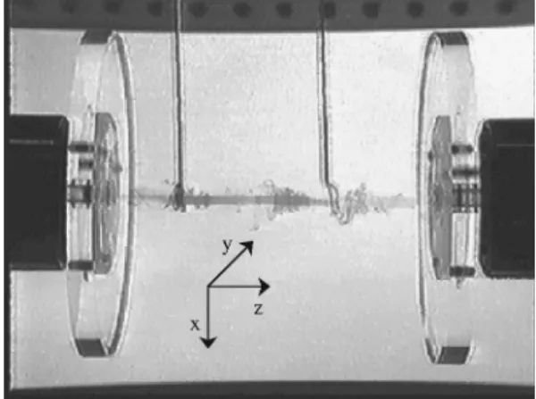
II. EXPERIMENTAL SETUP AND ACOUSTIC TECHNIQUE Our experiments rely on the transmission of an acoustic wave through a very thin and very intense vortex. Such a vorticity filament is generated in water between two coaxial, corotating disks 共diameter 10 cm兲, a classical von Ka´rma´n geometry关30兴. At the center of each disk, a symmetric suc-tion is applied by pumping the water through small holes of diameter 5 mm. The suction enhances the vorticity induced by the disk rotation, which generates a strong vorticity fila-ment between the two disks. The walls of the water tank are far enough from the disks so that the only control parameters are the disk rotation speed ⍀/2␲⫽0 – 20 Hz, the suction flow rate Q⫽0 – 6.4 l/min, and the distance between the two disks D⫽2 – 30 cm. The geometry of the experiment is sketched in Fig. 1. For more technical details about this hy-drodynamic setup, the reader is referred to Refs. 关31,32兴. In any case, the water level above the vortex axis is large enough to prevent any degassing or cavitation. In particular, we checked that no air bubble was present inside the vortex core, so that the vorticity filament generated with this setup is always acoustically penetrable. Figure 2 shows a snapshot of the vortex visualized by injecting dyes directly inside the vortex core.

Let us now briefly recall the transmission technique used to characterize a vortex with ultrasound 关7,8兴. As shown in Fig. 1共b兲, a plane wave is emitted by a linear array of 64 piezoelectric transducers working at a central frequency of f0⫽3.5 MHz. The element size is 0.39 mm along the x axis

by 12 mm along the z axis, and the transducers are prefo-cused in the z direction at 70 mm. The array pitch is 0.42

mm, leading to a total aperture of 27 mm. Each transducer has its own amplifier, an 8-bit digital-to-analog converter, a storage memory, and an 8-bit analog-to-digital converter working at 20 MHz. The plane wave propagates perpendicu-larly to the vortex axis in the 共xy兲 plane and keeps a rather small extent共less than 10 mm兲 in the z direction because of the prefocusing. The experimental configuration is thus close to the 2D situation classically investigated in theoretical papers.

The acoustic signal p(x,t) is recorded on another trans-ducer array after one crossing of the flow as a function of time t and of the receiver position x. This signal is compared to the one obtained in the fluid at rest, p0(x,t), using a

Fourier transform at the central frequency f0:

pˆ共x, f0兲

pˆ₀共x, f₀兲 ⫽A共x兲e

i␾共x兲_{, 共2.1兲}

where the caret indicates the Fourier transform. Equation 共2.1兲 defines the amplitude distortion A(x) and the phase distortion␾(x) of the acoustic wave due to the vortex. Both the Fourier transforms in Eq.共2.1兲 are taken in the same time window. Moreover, this window is chosen to fit only the transmitted signal in order to remove spurious echoes corre-sponding to reflections at the tank boundaries. Since the transducers can work in both transmit and receive modes, simultaneous two-way transmissions are systematically used to compensate for the effects of temperature or density inho-mogeneities in the medium and for possible mechanical vi-brations of the setup 关8,9,31兴. The positions of the two ar-rays, in particular their distances to the z axis, are controlled by 3D MicroControˆle actuators. In Sec. V, we will also use a monoelement transducer to emit a cylindrical wave at 3.5 or 1.5 MHz. In that case, the phase and amplitude distortions are still defined by Eq.共2.1兲 but two-way transmissions are no longer possible. All the acoustic measurements are per-formed in the plane z⫽D/6 rather than at z⫽0. Indeed, the stagnation point at z₀⬇0 关defined as the point on the z axis where the longitudinal velocity uz(z0) is zero兴 fluctuates

rap-idly in time and the flow may present strong three-dimensional features in the plane z⫽0.

FIG. 1. Sketch of the experimental setup共a兲 in the (y,z) plane;

共b兲 in the (x,y) plane: the incident plane wave emitted by the

trans-ducer array on the left is distorted and scattered by the vorticity filament.

FIG. 2. Photograph of the vorticity filament visualized with two different dyes. The two vertical lines correspond to the dye injectors.

The vorticity filament evolves on characteristic time scales of order 0.1 s, which are very long compared to the acoustic travel time over the distance L between the two transducer arrays and to the duration of emission 共typically 10␮s兲. Therefore, in the following, the flow will be consid-ered as frozen during one acoustic transmission. The propa-gation of sound through the vorticity filament can then be described in terms of two independent dimensionless param-eters:

M⫽u

c and ␤⫽ a

␭. 共2.2兲

M is the Mach number of the flow, u the maximum tangen-tial velocity of the vortex, and c⬇1500 m/s the speed of sound in water. ␤is the ratio of the vortex radius a to the acoustic wavelength␭⬇0.4 mm at 3.5 MHz and ␭⬇1 mm at 1.5 MHz. By convention, the vortex radius is defined by

u_␪共a兲⫽max关u_␪共r兲兴⫽u, 共2.3兲 where u_␪denotes the tangential velocity and r the distance to the center of the vortex.

In our experiments, u⬇1 m/s and a⬇1 mm so that M ⬇10⫺3 _{and␤⬇1 – 3. Thus, low Mach number}

approxima-tions will hold throughout this paper, whereas neither the Born limit (␤Ⰶ1) nor the geometrical acoustics approxima-tion (␤Ⰷ1) are valid here. In other words, when using our acoustic technique, we expect to observe both the effects of sound scattering by the vortex core and the long-range ef-fects of the velocity field on the incident wave.

III. ACOUSTIC MEASUREMENT OF THE VORTEX CIRCULATION

Outside the vortex core, i.e., for r⬎a, the flow is nearly irrotational and almost two dimensional. The velocity field should thus be given by u(r)⫽⌫/2␲re_␪, where ⌫ is the vortex circulation and e_␪ is the tangential unit vector. This behavior was checked in previous experiments in similar ge-ometries关9,33,34兴. Such a velocity field is slowly variable in space and sound-vortex interaction may be accounted for in the framework of geometrical acoustics. Let us denote as

n(r) the unit vector tangential to the acoustic ray at position r. The presence of the flow leads to a local modification of

the sound speed according to c(r)⫽c0⫹u(r)•n(r), where

c0is the sound speed in water at rest. If the acoustic ray does

not penetrate the vortex core, its direction is constant and equal to n(r)⫽ey for a plane wave propagating along the y

axis关35兴.

For small Mach numbers, using an expansion to first order in M, the phase distortion due to the vorticity filament is readily shown to be 关22兴 ␾共x兲⬇2␲_cf0 0 2

冕

冉

冊

shows the typical phase distortion

具

典

1024 consecutive samples. The distance between the two transducer arrays is L⬇200 mm and the incoming frequency is f0⫽3.5 MHz. The origin x⫽0 was chosen so that it

coin-cides with the average position of the vortex center:

具

典

corre-sponds to a signal that has been sped up共slowed down兲 by the flow. For 兩x兩⬎10 mm, i.e., outside the vortical region, the phase shift remains constant. Indeed, when 兩L/2x兩Ⰷ1, Eq. 共3.1兲 becomes ␾(x)⫽sgn(x)␲f0⌫/c0

2

. The phase jump ⌬␾between x⬍⫺10 mm and x⬎10 mm is thus given by

⌬␾⫽2␲f0

c₀2 ⌫. 共3.2兲

Using Eq. 共3.2兲, the vortex circulation is easily measured within a few percent. The measurements of Fig. 3共a兲 lead to ⌫⫽330⫾10 cm2_/s.

Note that in the Rankine model, for which u_␪(r) ⫽⌫/2␲r for r⭓a and u_␪(r)⫽⌫r/2␲a2 for r⭐a, ⌫ ⫽2␲ua so that

⌬␾

2␲⫽2␲M␤⬅␣. 共3.3兲

␣measures the amplitude of the phase jump and is called the ‘‘dislocation parameter.’’ When ␣⬎1, the wave front is ‘‘dislocated’’ in the sense that the vortex is strong enough to distort the wave front by more than one wavelength. In that case, additional wave fronts appear in the pressure field to compensate for such large phase jumps. The value of⌫ in-ferred from Fig. 3共a兲 corresponds to a rather small value of the dislocation parameter ␣⬇0.05. Our experimental situa-tion is thus slightly different from the one investigated by Vivanco et al.关20兴, where high values of the dislocation pa-rameter (␣⬇1) are achieved using surface waves.

As shown in Fig. 3, the fluctuations of the phase distortion around

具

典

fluctua-tions are much larger than the noise level of the data and can be attributed to the nonstationarity of the flow关31兴. Indeed, FIG. 3. 共a兲 Average phase distortion具␾(x)典tin the presence of a vorticity filament. The gray scale corresponds to the probability of observing a given value of ␾ around the mean measurement. 共b兲 Probability density function 共PDF兲 of ␾(x⫽⫺1 mm) 共䊉兲. The solid curve is a Gaussian fit of the experimental PDF. The experi-mental conditions are 1024 plane emissions at f0⫽3.5 MHz, L ⬇200 mm, ⍀/2␲⫽5.0 Hz, Q⫽3.7 l/min, and D⫽80 mm.

the vorticity filament constantly undergoes a more or less regular precession motion around the rotation axis of the disks. This precession motion depends on the control param-eters and can be studied using acoustics by following the position of the vortex关32兴. Moreover, the Reynolds number based on the disk radius can reach values as high as 105 so that some part of the flow may be turbulent even if the vortex always remains coherent. It is therefore not surprising to ob-serve a Gaussian statistics for the phase fluctuations关see Fig. 3共b兲兴.

The next section will show how important it is to com-pensate for the vortex motion in order to interpret correctly the phase distortion for兩x兩⬍10 mm. However, the raw aver-age

具

典

the vortex as a function of the control parameters ⍀ and D, as shown in Fig. 4. Those results show that

⌫⬀⍀

0.75

D0.5 . 共3.4兲

The power law dependence on⍀, with an exponent close to

3

4 for ⍀⫽0.5– 10 Hz, differs from the behavior as ⍀

1/2

pre-dicted and observed in confined flows关33,36兴. However, it is consistent with the results of Ref. 关37兴 obtained with counter-rotating disks, which show that ⌫⬀⍀0.8. The fact that ⌫ scales as D⫺1/2over the range D⫽20– 80 mm can be explained by simple energetic considerations 关32兴. The de-parture from the power law behavior for larger values of D results from an instability of the vorticity filament. Indeed, when the distance between the disks is increased, the vortex may undergo breakdowns that lead to a lower mean circula-tion.

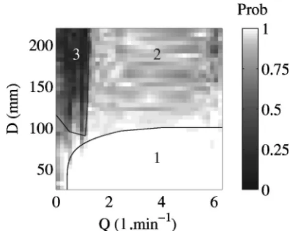
In order to track such an instability in the control param-eter space, we define a ‘‘probability of presence’’ of the vortex by counting the proportion of phase measurements that display a phase jump similar to that of Fig. 3共a兲. Such phase distortions are characteristic of the presence of a vor-ticity filament. For a given set of control parameters, the probability of presence is computed from 1024 measure-ments recorded in about 2 min. Such a sample is long enough to yield a good statistical characterization of the vor-ticity filament. The resulting stability diagram in the (Q,D)

plane is shown in Fig. 5 for a given value of ⍀. Three dif-ferent domains can be qualitatively distinguished. When the suction is large and the disks are close to each other (D ⬍100 mm), the probability of presence is 1 共domain 1兲. However, the probability decreases down to values of order 0.5 when Q is decreased or when D is increased共domain 2兲. In that case, the vorticity filament goes unstable from time to time and the phase distortion does not always display a phase jump. A very sharp transition is observed between domain 2 and domain 3 where the vorticity filament almost never shows up. Indeed, when the suction is too weak and the distance D too large, the vorticity injected in the flow by the disk rotation is not amplified to form a vorticity filament and jumps are never observed in the phase distortion.

Lastly, the vortex circulation can be measured from the phase distortions as a function of time. Such dynamical mea-surements were performed with a 30 Hz sampling rate in the case of the transient regime of formation of the vorticity filament. Figure 6共a兲 presents a spatiotemporal diagram of the phase measurements after the rotation and the suction are applied simultaneously at time t₀⫽6 s. The phase distortion goes from zero to the typical phase jump within about 5 s. Figure 6共b兲 shows that the wave front is first only bent due to

FIG. 4. Mean circulation of the vorticity filament as a function of 共a兲 the rotation speed of the disks ⍀ 共for Q⫽3.0 l/min and D

⫽120 mm) and 共b兲 the distance D between the two disks 共for ⍀/2␲⫽1.7 Hz and Q⫽5.5 l/min). Note the logarithmic scales and

the error bars, which represent the data standard deviation. Solid lines correspond to power laws with exponents 0.75 and⫺0.5.

FIG. 5. Stability diagram of the vorticity filament in the (Q,D) plane. The gray scale corresponds to the probability of presence of the vorticity filament computed from 1024 consecutive measure-ments of the phase distortion for⍀/2␲⫽0.8 Hz.

FIG. 6. Transient regime during the formation of the vorticity filament.共a兲 Phase distortions␾(x) measured as a function of time and coded in gray levels.共b兲␾(x) at t⫽6.5 共䊉兲, 9.8 共䉭兲, and 13.1 s 共䊏兲. ⍀/2␲⫽6.7 Hz, Q⫽5.7 l/min, and D⫽80 mm. Rotation and suction are turned on at t0⫽6 s.

the solid body rotation induced by the disk rotation. The vorticity is then amplified by the pumping and concentrates in the vortex core to form the vorticity filament. For t ⬎15 s, after the transient regime, the precession motion of the vortex can be detected in the fluctuations of␾(x). Figure 7 displays the evolution of the vortex circulation ⌫(t) de-duced from the phase measurements during various transient regimes of formation. In Figs. 7共a兲 and 7共b兲, the rotation speed⍀ of the disks is varied for a fixed suction flow rate Q, whereas, in Figs. 7共c兲 and 7共d兲, Q is varied for a given value of ⍀. For each set of control parameters, the curve ⌫(t) is well fitted by an exponential relaxation, which defines a characteristic growth time␶for the circulation. Figures 7共b兲 and 7共d兲 show that␶is almost independent of⍀ but strongly decreases with Q. Even if rotation and stretching are never completely independent 关36兴, this result means that in this experiment the formation of the vorticity filament is mainly governed by the suction flow rate. The rotation thus dictates only the asymptotic value ⌫0 of the circulation 关compare

Figs. 7共a兲 and 7共c兲兴. Indeed, from the vorticity equation, one gets关38兴

⳵␻z

⳵t ⬇␻z

⳵uz

⳵z , 共3.5兲

where␻z is the component of the vorticity␻⫽“⫻u along

the z axis. The ‘‘stretching’’ ␥⫽⳵uz/⳵z appears as the

in-verse of a characteristic time. A rough estimate for the

stretching is ␥⬀2uz(z⫽D/2)/D⬇Q/DS, where S denotes

the surface of the suction hole. Since ␶⬀1/␥, one expects that ␶⬀D/Q, in good agreement with Fig. 7共d兲, where ␶ is shown to scale as 1/Q for large value of Q. Once again, for the smallest flow rates, the vortex may be unstable so that

␶(Q) may depart from this simple behavior.

IV. SCATTERING OF A PLANE WAVE

In the previous section, we used an approach based on geometrical acoustics to account for the phase jump ⌬␾. This approach is valid outside the vortex core where the flow is slowly varying in space. Here, we show that this first ef-fect 共the phase jump兲 goes along with an effect due to scat-tering of the incoming ultrasound by the vortex core.

As previously mentioned in Refs. 关20,22兴, sound scatter-ing leads to oscillations in the phase distortion that are su-perimposed on the phase jump. Those oscillations can be interpreted as an interference pattern between the distorted incident wave and the scattered wave. In the present experi-ment, the very small radius of the vortex should allow sound scattering to take place. However, oscillations are not clearly visible in the raw average

具

典

to the precession motion of the vortex, oscillations cancel out when the phase measurements are averaged over 1024 samples without any further data analysis. In order to take into account the precession motion, we first measure the po-sition of the vortex center along the x axis. This popo-sition is obtained from each phase measurement ␾ by detecting the abscissa x0 for which ␾(x0)⫽0. This procedure yields a

time series x₀(t) and the phase distortions are then aver-aged in the vortex frame of reference by computing FIG. 7. Transient regimes of formation. 共a兲 Vortex circulation

⌫(t) for ⍀/2␲⫽2.1 Hz 共gray兲 and ⍀/2␲⫽6.7 Hz 共black兲. Solid

lines are exponential fits of the form ⌫(t⫹t0)⫽⌫0关1⫺exp(⫺t/␶)兴

with ␶⫽5.0 and 4.7 s, respectively. ⌫0 is the final value of the

circulation. 共b兲 Characteristic time ␶共⍀兲 for Q⫽5.7 l/min and D

⫽80 mm. 共c兲 ⌫(t) for Q⫽0.7 共gray兲 and 6.3 l/min 共black兲. The

solid lines are computed with␶⫽17 and 9 s, respectively. 共d兲 ␶(Q) for ⍀/2␲⫽0.8 Hz and D⫽80 mm. The solid line represents a fit with ␶⬀1/Q. Rotation and suction are turned on at t0⫽6 s in 共a兲

and 8 s in共b兲.

FIG. 8. Compensation of the vortex motion. 共a兲 Mean phase distortion 具␾„x⫺x0(t)…典t and 共b兲 mean amplitude distortion 具A„x⫺x0(t)…典t averaged in the vortex frame of reference. 共c兲 具␾„x⫺x0(t)…典t 共䊉 and black line兲 compared to具␾(x)典t 共䊊 and gray line兲. 共d兲 具A„x⫺x0(t)…典t 共䊉 and black line兲 compared to 具A(x)典t共䊊 and gray line兲. Same experimental conditions as in Fig. 3.

具

典

both the phase and the amplitude distortions when such a dynamical analysis is applied to the experimental data. In Figs. 8共c兲 and 8共d兲, averaging in the vortex frame of refer-ence is compared to the raw averaging used in Fig. 3共a兲. Even if the values reached far from the vortex core are the same, the signals are much smoother and the oscillations much better defined when one compensates for the vortex motion.

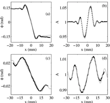
Analytical calculations are available for the scattering of an infinite plane wave generated at infinity and incident on a Rankine vortex 关19,21兴 or, equivalently, for scattering by a penetrable tube of magnetic field关39兴. Such calculations are compared to experimental data in Fig. 9. The distance Lem

(L_rec) between the z axis and the emitter共receiver兲 array is tuned to Lrec⫽Lem⫽L/2⫽120 mm. The vortex circulation ⌫

is first measured from the phase jump as in Sec. III. Thus, the only adjustable parameter in the analytical calculation is the vortex radius a. Very good fits of both the phase and ampli-tude distortions are obtained with a⫽1.3⫾0.1 mm, which corresponds to ␤⬇3. Note that such a measurement of the size of the vortex core is impossible with standard hot wire probes and would be very difficult with Doppler techniques due to particle demixing in the core 关34兴.

In the far field region and outside an angular sector around the forward direction, more precisely for (2␲kr)1/2 Ⰷ1 and ␲⫺兩␪兩Ⰷ1/(kr)1/2_{, the analytical expression of the}

pressure field reduces to关19兴

p共r,␪兲⬀e⫺ikr cos␪⫹i␣␪⫹F共␪兲sin共␲␣兲 e

ikr

冑

where F(␪)⫽exp(i␪/2)/i cos(␪/2). k is the wave number and

␪the polar angle between⫺eyand the direction of

observa-tion r. The first term of the sum in Eq. 共4.1兲 describes the distortion of the plane incident wave: the phase term ␣␪ corresponds exactly to the phase distortion given by Eq. 共3.1兲. The second term represents the scattered wave and leads to the oscillations in ␾(x) and A(x).

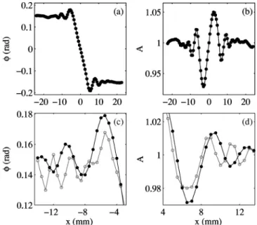
V. SCATTERING OF A CYLINDRICAL WAVE The above interpretation in terms of interference between the incident wave and the scattered wave still holds for a cylindrical incident wave. Due to the large aspect ratio of our transducers (⬇0.5⫻10 mm2), we shall assume that the acoustic field emitted by a single transducer is mainly two dimensional and call it ‘‘cylindrical.’’ Figure 10 compares the experimental results obtained at f0⫽3.5 MHz with plane

and cylindrical incident waves. Due to the divergent nature of the cylindrical wave, the wavelength of the oscillations in the wave-front distortion is bigger than with a plane wave. Moreover, the use of a single emitting element allows us to use a receiver array of 127 transducers with a pitch of 0.42 mm. The number of experimental points per oscillation is thus larger with a cylindrical emission 关Figs. 10共c兲 and 10共d兲兴 than with a plane emission 关Figs. 10共a兲 and 10共b兲兴. In other words, a cylindrical emission provides a ‘‘zoom’’ on the vortex core and may lead to better precision in estimation of the vortex size.

However, to our knowledge, no analytical calculation is available in the literature in the case of a cylindrical wave emitted at a finite distance from a vortex. In order to interpret our data, we were led to implement a monochromatic nu-merical simulation based on a 2D parabolic equation. Previ-ous numerical studies using parabolic equations dealt with the well-documented case of a plane incident wave关40,41兴. Our numerical code was described and tested in a previous paper 关42兴. It relies on the resolution of the inhomogeneous Helmholtz equation

ⵜ2_p⫹k2_{共r兲p⫽S共r兲, 共5.1兲}

where S(r) corresponds to the acoustic sources and the local wave number k(r)⫽2␲f0/关c0⫹u(r)•n(r)兴 results from the

FIG. 9. Comparison between experimental data共䊉兲 averaged in the vortex frame of reference and the analytical calculations for⌫

⫽145 cm2

/s and a⫽1.3 mm 共gray lines兲. 共a兲 Phase distortion. 共b兲 Amplitude distortion. The experimental conditions are 1024 plane emissions at f0⫽3.5 MHz, L⫽240 mm, ⍀/2␲⫽1.7 Hz, Q⫽5.9

l/min, and D⫽80 mm.

FIG. 10. Influence of the incident wave form.共a兲 Phase and 共b兲 amplitude distortions averaged in the vortex frame of reference for a plane incident wave and共c兲, 共d兲 for a cylindrical incident wave. The experimental conditions are 4096 emissions at f0⫽3.5 MHz,

sound-flow interaction. This expression for k(r) is valid for small Mach numbers and for ␤Ⰷ1/2␲. Equation 共5.1兲 is solved in the forward direction y⬎0 using the parabolic equation

⳵p

⳵y⫽ik0

冑

The numerical scheme uses the split-step Pade´ solution pro-posed by Collins关43兴. Higher-order Pade´ approximations of 关1⫹K(r)兴1/2 _{provide a good numerical convergence for}

propagation angles up to 85° away from the y axis. The first-order differential equation共5.2兲 is solved from the emis-sion plane y⫽⫺Lemto y⫽Lrecwith a step␦y⫽␭. The

dis-cretization along the x axis is ␦x⫽␭/10. The fluid velocity field is a Burgers vortex

u_␪共r兲⫽ ⌫ 2␲r共1⫺e ⫺r2_/4r 0 2 兲, 共5.3兲

where r0 is proportional to the vortex radius a⬇2.24r0 and

is given by r0⫽(␯/␥)1/2, where␯is the fluid kinematic

vis-cosity and␥is the stretching. For a cylindrical wave emitted at position R, the direction of propagation is taken to be

n(r)⫽(r⫺R)/储r⫺R储 even in the presence of the vortex.

This assumption is valid provided that MⰆ1.

The cylindrical wave is emitted from R⫽⫺L_eme_y. The phase and amplitude distortions are computed at y⫽Lrec

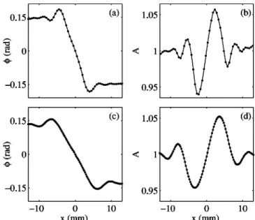
from the pressure fields simulated in the presence of a vor-ticity filament and in the fluid at rest. By tuning ⌫ and a, a very good agreement with the experiment is obtained, as shown in Fig. 11 for f0⫽3.5 and 1.5 MHz. The

characteris-tics of the vortex are estimated within ⫾5%. Due to the larger wavelength and smaller vortex size, the measurements at f0⫽1.5 MHz correspond to␤⬇1. This value constitutes a

physical limit of resolution of our technique. Indeed, we checked that for vortices of constant circulation but of dif-ferent sizes below the acoustic wavelength (␤⭐1), the wave-front distortions are very close to each other. In par-ticular, the amplitude of the oscillations saturates, so that

␾(x) and A(x) vary significantly only for␤⭓1.

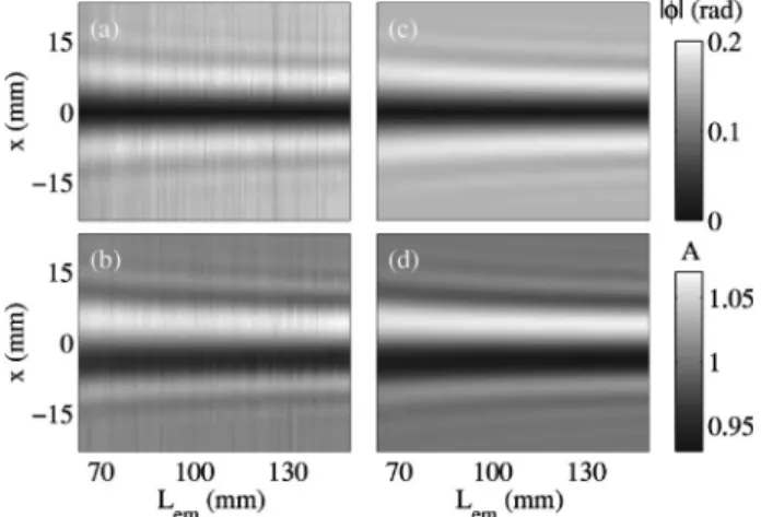
The agreement between the simulation and the experi-ment is confirmed in Figs. 12 and 13 where the distances L_rec and Lemare successively varied. Varying Lrec共Fig. 12兲 gives

a picture of the wave-front distortion in two dimensions as the receiver gets farther from the vortex. Varying L_em共Fig. 13兲 helps to understand the convergence of the case of a cylindrical emission toward the case of a plane emission. Indeed, one expects that the results obtained with a plane incident wave will be recovered when Lem→⬁. Moreover, it

is reasonable to assume that the far field solution takes a simple expression similar to Eq. 共4.1兲. Let us postulate that, for (2␲kr)1/2_{Ⰷ1 and ␲⫺兩␪兩Ⰷ1/(kr)}1/2_{, the pressure field}

can be written as the sum of a distorted cylindrical wave and a scattered wave. By using Eq. 共3.1兲 and 养u•dl⫽0 for a given closed path inside the irrotational region of the flow, it is easy to show that the phase distortion of a cylindrical wave is independent of Lem and is given by ␣␪ as in the plane

wave case. Taking into account the attenuation of the inci-dent wave with distance leads to the following expression for the pressure field:

p共r,␪兲⬀e

⫺ikr⬘⫹i␣␪

冑

⬘

冑

⬘

ac-FIG. 11. Comparison between experimental data共䊉兲 averaged in the vortex frame of reference and the parabolic equation simula-tion共gray lines兲. 共a兲 Phase and 共b兲 amplitude distortions for a cy-lindrical emission at f0⫽3.5 MHz with L⫽180 mm, ⍀/2␲ ⫽5.0 Hz, Q⫽3.7 l/min, D⫽80 mm, and disks of diameter 10 cm.

Simulation for a Burgers vortex关Eq. 共5.3兲兴 with ⌫⫽310 cm2/s and a⫽1.35 mm. 共c兲 Phase and 共d兲 amplitude distortions for a cylindri-cal emission at f0⫽1.5 MHz with L⫽210 mm, ⍀/2␲⫽3.0 Hz, Q ⫽3.1 l/min, D⫽30 mm, and disks of diameter 5 cm. Simulation

with⌫⫽112 cm2_{/s and a⫽0.9 mm.}

FIG. 12. Influence of the receiver position for a cylindrical emission at f0⫽3.5 MHz. 共a兲 Experimental phase and 共b兲 amplitude

distortions with Lem⫽90 mm, ⍀/2␲⫽5.0 Hz, Q⫽3.7 l/min, D ⫽80 mm. 共c兲, 共d兲 Simulation with ⌫⫽325 cm2

count for this dependence is to take G(␪,Lem)

⫽F(␪)/(2i␲kLem)1/2where F(␪) is given in Sec. V. Such a

dependence means that the scattered wave is the same as in the plane wave case. Its amplitude has only been rescaled by the amplitude of the incident wave at r⫽0 共using r

⬘

r⫽0). As shown in Fig. 14, Eq. 共5.4兲 provides a rather good prediction for the oscillations in ␾(x) and A(x). Since r

⬘

Eq. 共5.4兲 should tend toward the plane wave case as Lem

→⬁. However, the oscillations predicted by Eq. 共5.4兲 are

slightly out of phase with the results of the simulation for large values of x. This may indicate that G also depends on the vortex radius a and that the variation of the curvature of the incident wave front with size a plays a significant role.

VI. NUMERICAL INVESTIGATION OF THE SCATTERED WAVE

The parabolic equation used in the previous section al-lows us to account for scattering around the forward direc-tion. It is thus very well suited for modeling our transmission

ing medium. Our approach discriminates between a station-ary, incompressible basic flow (u, P0,␳0) and an acoustic

perturbation (v, p,␳). The density of the basic flow is as-sumed to be constant and the acoustic pressure and density are linked by the equation of state p⫽␳c₀2. Linearizing the Navier-Stokes equations and neglecting all terms of order M2 lead to the following coupled equations关47兴:

ⵜ2_p⫺ 1 c0 2 ⳵2_p ⳵t2⫽⫺2␳0 ⳵2 ⳵xi⳵xj共ui vj兲⫹S共r,t兲, 共6.1a兲 ⳵v ⳵t⫹共u•“兲v⫹共v•“兲u⫽⫺ “p ␳0 . 共6.1b兲

In Eq. 共6.1a兲, the sound-flow interaction appears as a source term which involves the acoustic velocity v. Thus, the problem has to be solved for both the variables p and v. The 2D version of Eq.共6.1兲 is discretized over a rectangular grid of mesh ␦x⫽␦y⫽␭/12 with 210⫻210 points. The time step is ␦t⫽1/20f0, so that the von Neumann stability criterion

␦t⭐␦x/c0& is satisfied. A second-order scheme is used to

estimate the derivatives in Eq. 共6.1a兲. Higher-order absorb-ing boundary conditions as in Ref. 关48兴 limit the amplitude of waves reflected at the grid boundaries to⫺45 dB.

It can be shown that Eq.共6.1兲 is valid for␤ⰇM/2␲ 关31兴. Since MⰆ1, it is more general than Eq. 共5.1兲. In the mono-chromatic regime and when ␤Ⰷ1/2␲, Eqs. 共6.1兲 and 共5.1兲 are equivalent and we checked that the results obtained in the forward direction with the parabolic equation and with the finite-difference code coincide. In spite of much longer com-putation times, the advantage of the finite-difference ap-proach is to give access to the pressure field in time and for any direction of propagation. Figure 15 shows the propaga-tion of a cylindrical pulse p(x, y ,t) through a Burgers vortex for M⫽0.1 and␤⫽0.5. As seen in Figs. 15共b兲 and 15共c兲, the incident wave front is clearly distorted by the vortex core. The scattered wave is small compared to the incident pres-sure and can hardly be observed in Fig. 15共c兲.

A standard way to focus on the scattered wave is to study the difference pscatt⫽p⫺p0, where p0 is the reference

acoustic pressure computed in the fluid at rest. This is sup-posed to get rid of the incident wave front pinc⬇p0.

How-ever, as shown in Figs. 15共d兲–15共f兲, this definition does not allow a better observation of the wave scattered by a Burgers vortex. Indeed, pscattcontains not only the contribution of the

scattered wave but also the effects of the advection due to the long-range nature of the Burgers velocity field u_␪(r)⬃1/r as r→⬁. This explains why pscattis always of the order of the

incident pressure: even before the incident pulse crosses the vortex, p⫽p0due to advection effects关Fig. 15共d兲兴. Note that

in Ref. 关44兴 those effects are referred to as ‘‘refraction’’ FIG. 13. Influence of the emitter position for a cylindrical

emis-sion at f0⫽3.5 MHz. 共a兲 Experimental phase and 共b兲 amplitude

distortions with Lrec⫽90 mm, ⍀/2␲⫽5.0 Hz, Q⫽3.7 l/min, D ⫽80 mm. 共c兲,共d兲 Simulation with ⌫⫽325 cm2_{/s and a⫽1.35 mm.}

FIG. 14. Comparison between the parabolic equation simulation with⌫⫽470 cm2_{/s and a⫽0.5 mm 共gray lines兲 and the prediction}

of Eq.共5.4兲 with␣⫽0.03 共black solid and dashed lines兲. 共a兲 Phase and 共b兲 amplitude distortions for a cylindrical emission at f0 ⫽1.5 MHz with Lem⫽50 mm and Lrec⫽200 mm. The dashed lines

are linear interpolations for the values of x where Eq. 共5.4兲 is not valid.

effects, which is rather ambiguous since the flow is irrota-tional for r⬎a and acoustic rays are not deflected by irrota-tional flows. In Fig. 15共f兲, the effects of advection mask the scattered wave, which is about 100 times smaller. Let us finally mention that advection also affects the scattered wave at large distances from the vortex core.

In order to avoid such effects of a slowly decaying veloc-ity field, one may use a vortex with vanishing circulation. As mentioned by Colonius, Lele, and Moin关44兴, the Taylor vor-tex, whose velocity field decays exponentially fast,

u_␪共r兲⫽ur aexp

冋

冉

冊册

scattered away from a Taylor vortex. It is clear that the

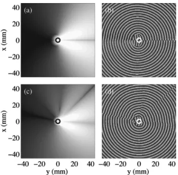
scat-tered amplitude around the forward direction is much larger than that of the backscattered signal. Moreover, for M ⫽0.1, the scattered wave is not symmetric about the y axis. Finite-difference schemes also allow one to study the 共quasi兲monochromatic regime by using much longer emis-sions. Figure 17 presents the amplitude and the phase of the scattered pressure field pscattfor a monochromatic cylindrical

wave incident on a Taylor vortex. According to Ref.关44兴, we expect these results to be very close to those given by Light-hill’s acoustic analogy 关11兴. For very small Mach numbers, the scattered amplitude displays a classical, quadrupolar pat-tern关Fig. 17共a兲兴. Outside a line of singularity in the forward direction, where p_scatt vanishes, the phase in Fig. 17共b兲 re-veals that the scattered wave has a cylindrical structure as expected from theoretical and analytical approaches关11–17兴. When M is increased for a given value of ␤, the scattered amplitude becomes asymmetric 关Fig. 17共c兲兴. Moreover, Fig. 17共d兲 shows that the scattered wave for M⫽0.1 has a spiral structure. This feature was not pointed out in previous nu-merical studies, which focused on rms pressure levels or on directivity patterns 关40,44兴. Our simulation also reveals the presence of two defects in the phase pattern before the spiral wave fully develops in space. Such spiral solutions of the scattering problem have been predicted theoretically by Umeki and Lund 关49兴 and observed experimentally in the interaction between surface waves and a vortex 关50兴. In the case of a finite-circulation vortex, such spiral waves are likely to be favored by the long-range advection effects that strongly distort the scattered wave at ‘‘large’’ Mach num-bers. The present numerical results obtained for␣⫽0.3 and FIG. 15. Propagation of a cylindrical pulse through a Burgers

vortex关Eq. 共5.3兲兴 with M⫽0.1 and␤⫽0.5. Acoustic pressure field p(x,t) at t⫽(a)55, 共b兲 80, and 共c兲 105␮s. ‘‘Scattered’’ pressure field pscatt⫽p⫺p0at t⫽(d) 55, 共e兲 80, and 共f兲 105␮s. The vortex

rotates clockwise and its center is indicated by a white circle. The cylindrical wave共eight acoustic periods at f0⫽500 kHz) is emitted

from Lem⫽⫺75 mm. The pressure is coded using a linear gray

scale. In共a兲–共c兲, black corresponds to the minimum pressure and white to the maximum pressure. In共d兲 and 共e兲, pscatthas been

res-caled by the maximum value obtained in共f兲.

FIG. 16. Propagation of a cylindrical pulse共eight acoustic peri-ods at f0⫽500 kHz) through a Taylor vortex 关Eq. 共6.2兲兴 with M ⫽0.1 and ␤⫽0.5. ‘‘Scattered’’ pressure field pscatt⫽p⫺p0 at t ⫽(a) 55, 共b兲 80, and 共c兲 105 ␮s. In 共a兲 and 共b兲, pscatt has been

rescaled by the maximum value obtained in共c兲.

FIG. 17. Pressure field scattered by a Taylor vortex for a mono-chromatic cylindrical incident wave.共a兲 Amplitude and 共b兲 phase of

pscattfor M⫽10⫺4and␤⫽0.5. 共c兲 Amplitude and 共d兲 phase of pscatt

for M⫽0.1 and␤⫽0.5. The cylindrical wave 共40 acoustic periods at f0⫽500 kHz) is emitted from Lem⫽⫺75 mm. The amplitude is

coded using a logarithmic gray scale: white is⫺10 dB and black is

⫺180 dB in 共a兲 and ⫺120 dB in 共c兲 relative to the maximum value

3⫻10⫺4with␤⫽0.5 constitute a useful complement to the analytical calculations by Coste, Lund, and Umeki 关21兴, valid for ␣⬇1 and␤Ⰷ1/2␲.

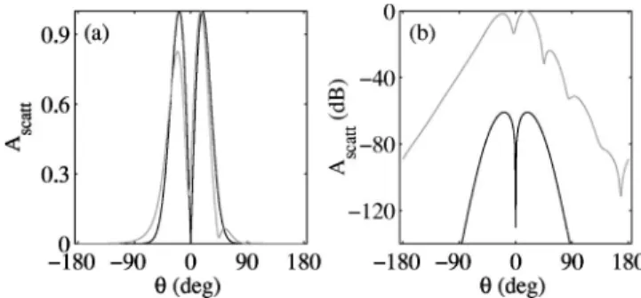
Finally, the directivity patterns corresponding to Figs. 17共a兲 and 17共c兲 are plotted in Fig. 18. Not surprisingly, they are very similar to those obtained in Refs. 关40,44兴 with a plane illumination. The peak scattering occurs at about ␪⫽ ⫾20° from the forward direction. No backscattering is ob-served at low Mach numbers and a strong asymmetry shows up for M⫽0.1.

VII. CONCLUSIONS

The results presented in this paper are twofold. First, ex-perimental data on the interaction between an ultrasonic

measurements that turn out to be very interesting for study-ing transient regimes and the dynamics of vorticity.

Second, the case of a cylindrical incident wave has been studied in detail with a parabolic equation and a finite-difference numerical code. Such an investigation resulted from experimental motivations: cylindrical emission by a single element is cheaper, easier to control, does not require the use of two transducer arrays, and yields a more accurate measurement especially inside the vortex core. Our numeri-cal results are similar to those of Refs. 关21,40,44兴 but also uncover an original spiral solution for the scattered wave at ‘‘large’’ Mach numbers ( M⫽0.1 for␤⫽0.5). The crossover between cylindrical and spiral scattered waves as a function of M and␤is currently under study.

As a global conclusion, we stress that the analysis of ex-perimental data in the light of numerical simulations pro-vides useful results for both the problem of remote sensing of vorticity filaments and the theoretical understanding of sound scattering by a vortex.

ACKNOWLEDGMENTS

C. Baudet, Ph. Blanc-Benon, Y. Couder, F. Lund, J.-F. Pinton, and J.-E. Wesfreid are thanked for fruitful discus-sions.

关1兴 D. W. Schmidt and P. M. Tilmann, J. Acoust. Soc. Am. 47,

1310共1970兲.

关2兴 R. H. Engler, D. W. Schmidt, W. J. Wagner, and B.

Weite-meier, J. Acoust. Soc. Am. 71, 42共1982兲.

关3兴 W. Munk, J. Fluid Mech. 173, 43 共1986兲.

关4兴 W. Munk, P. Worcester, and C. Wunsch, Ocean Acoustic

To-mography共Cambridge University Press, Cambridge, 1995兲.

关5兴 R. H. Engler, D. W. Schmidt, and W. J. Wagner, J. Acoust.

Soc. Am. 85, 72共1989兲.

关6兴 A. Hauck, Acoust. Imaging 18, 317 共1991兲.

关7兴 R. Labbe´ and J.-F. Pinton, Phys. Rev. Lett. 81, 1413 共1999兲. 关8兴 S. Manneville, A. Maurel, P. Roux, and M. Fink, Eur. Phys. J.

B 9, 545共1999兲.

关9兴 S. Manneville, J.-H. Robres, A. Maurel, P. Petitjeans, and M.

Fink, Phys. Fluids 11, 3380共1999兲.

关10兴 S. Douady, Y. Couder, and M.-E. Brachet, Phys. Rev. Lett. 67,

983共1991兲.

关11兴 M. J. Lighthill, Proc. R. Soc. London, Ser. A 211, 564 共1952兲. 关12兴 A. L. Fetter, Phys. Rev. A 136, 1488 共1964兲.

关13兴 S. O’Shea, J. Sound Vib. 43, 106 共1975兲.

关14兴 A. L. Fabrikant, Akust. Zh. 28, 694 共1982兲 关Sov. Phys. Acoust.

28, 410共1982兲兴.

关15兴 P. V. Sakov, Akust. Zh. 39, 537 共1993兲 关Acoust. Phys. 39, 280 共1993兲兴.

关16兴 J. Reinschke, W. Mo¨hring, and F. Obermeier, J. Fluid Mech.

333, 273共1997兲.

关17兴 R. Ford and S. G. Llewellyn Smith, J. Fluid Mech. 386, 305 共1999兲.

关18兴 Y. Aharonov and D. Bohm, Phys. Rev. 115, 485 共1959兲. 关19兴 M. V. Berry, R. G. Chambers, M. D. Large, C. Upstill, and J.

C. Walmsley, Eur. J. Phys. 1, 154共1980兲.

关20兴 F. Vivanco, F. Melo, C. Coste, and F. Lund, Phys. Rev. Lett.

83, 1966共1999兲.

关21兴 C. Coste, F. Lund, and M. Umeki, Phys. Rev. E 60, 4908 共1999兲.

关22兴 P. Roux, J. de Rosny, M. Tanter, and M. Fink, Phys. Rev. Lett.

79, 3170共1997兲.

关23兴 J.-F. Pinton and G. Brillant 共private communication兲. 关24兴 D. Blockintzev, J. Acoust. Soc. Am. 18, 322 共1945兲. 关25兴 V. E. Ostashev, Acoustics in Moving Inhomogeneous Media 共E

& FN Spon, London 1997兲.

关26兴 R. H. Kraichnan, J. Acoust. Soc. Am. 25, 1096 共1953兲. 关27兴 F. Lund and C. Rojas, Physica D 37, 508 共1989兲.

关28兴 C. Baudet, S. Ciliberto, and J.-F. Pinton, Phys. Rev. Lett. 67,

193共1991兲.

关29兴 C. Baudet, O. Michel, and W. J. Williams, Physica D 128, 1 共1999兲.

FIG. 18. Scattering amplitude vs the angle with the forward direction for M⫽10⫺4 共black兲 and M⫽0.1 共gray兲 with␤⫽0.5. 共a兲 Linear scale.共b兲 Logarithmic scale in dB. The directivity diagrams have been taken from Figs. 17共a兲 and 17共c兲 at r⫽30 mm and res-caled by their own maximum in共a兲 and by the maximum amplitude obtained at M⫽0.1 in 共b兲.

关30兴 R. Labbe´, J.-F. Pinton, and S. Fauve, Phys. Fluids 8, 914 共1996兲.

关31兴 S. Manneville, Ph.D. thesis, University Paris 7, 2000. 关32兴 S. Manneville, A. Maurel, F. Bottausci, and P. Petitjeans,

Structure and Dynamics of Vortices, edited by A. Maurel and P. Petitjeans, Lecture Notes in Physics Vol. 555 共Springer-Verlag, Berlin, 2000兲, p. 231.

关33兴 M. Mory and N. Yurchenko, Eur. J. Mech. B/Fluids 6, 729 共1993兲.

关34兴 R. Wunenburger, B. Andreotti, and P. Petitjeans, Exp. Fluids

27, 181共1999兲.

关35兴 L. D. Landau and E. M. Lifshitz, Fluid Mechanics 共MIR,

Mos-cow, 1989兲.

关36兴 B. Andreotti, Ph.D. thesis, University Paris 7, 1999.

关37兴 N. Mordant, J.-F. Pinton, and F. Chilla`, J. Phys. II 7, 1729 共1997兲.

关38兴 P. G. Saffman, Vortex Dynamics 共Cambridge University Press,

Cambridge, 1992兲.

关39兴 S. Olariu and I. Iovitzu Popescu, Rev. Mod. Phys. 57, 339

共1985兲.

关40兴 S. M. Candel, J. Fluid Mech. 83, 465 共1979兲.

关41兴 V. E. Ostashev, D. Juve´, and P. Blanc-Benon, Acust. Acta

Acust. 83, 455共1997兲.

关42兴 P. Roux, H. C. Song, M. B. Porter, and W. A. Kuperman,

Wave Motion 31, 181共2000兲.

关43兴 M. D. Collins, J. Acoust. Soc. Am. 96, 382 共1994兲; 93, 1736 共1993兲.

关44兴 T. Colonius, S. K. Lele, and P. Moin, J. Fluid Mech. 260, 271 共1994兲.

关45兴 C. Bailly and D. Juve´, AIAA J. 38, 22 共2000兲. 关46兴 R. Berthet 共private communication兲.

关47兴 B. T. Chu and L. S. G. Kova´sznay, J. Fluid Mech. 3, 494 共1958兲.

关48兴 F. Collino, Institut National de Recherche en Informatique et

en Automatique Report No. 1790, 1993共unpublished兲.

关49兴 M. Umeki and F. Lund, Fluid Dyn. Res. 21, 201 共1997兲. 关50兴 F. Vivanco and F. Melo, Phys. Rev. Lett. 85, 2116 共2000兲.