Measurement depth effects on the apparent temperature sensitivity of soil respiration in field studies

(1)

HAL Id: hal-00298001

https://hal.archives-ouvertes.fr/hal-00298001

Submitted on 6 May 2008

HAL is a multi-disciplinary open access

archive for the deposit and dissemination of sci-entific research documents, whether they are pub-lished or not. The documents may come from teaching and research institutions in France or abroad, or from public or private research centers.

L’archive ouverte pluridisciplinaire HAL, est destinée au dépôt et à la diffusion de documents scientifiques de niveau recherche, publiés ou non, émanant des établissements d’enseignement et de recherche français ou étrangers, des laboratoires publics ou privés.

Measurement depth effects on the apparent temperature

sensitivity of soil respiration in field studies

A. Graf, L. Weihermüller, J. A. Huisman, M. Herbst, J. Bauer, H. Vereecken

To cite this version:

A. Graf, L. Weihermüller, J. A. Huisman, M. Herbst, J. Bauer, et al.. Measurement depth effects on the apparent temperature sensitivity of soil respiration in field studies. Biogeosciences Discussions, European Geosciences Union, 2008, 5 (3), pp.1867-1898. �hal-00298001�

(2)

BGD

5, 1867–1898, 2008 Temperature measurement depth effects A. Graf et al. Title Page Abstract Introduction Conclusions References Tables Figures ◭ ◮ ◭ ◮ Back Close Full Screen / Esc

Printer-friendly Version Interactive Discussion Biogeosciences Discuss., 5, 1867–1898, 2008

www.biogeosciences-discuss.net/5/1867/2008/ © Author(s) 2008. This work is distributed under the Creative Commons Attribution 3.0 License.

Biogeosciences Discussions

Biogeosciences Discussions is the access reviewed discussion forum of Biogeosciences

Measurement depth effects on the

apparent temperature sensitivity of soil

respiration in field studies

A. Graf, L. Weiherm ¨uller, J. A. Huisman, M. Herbst, J. Bauer, and H. Vereecken

Forschungszentrum J ¨ulich, Agrosphere Institute (ICG-4), Institute for Chemistry and Dynamics of the Geosphere, 52425 J ¨ulich, Germany

Received: 7 April 2008 – Accepted: 7 April 2008 – Published: 6 May 2008 Correspondence to: A. Graf (a.graf@fz-juelich.de)

(3)

BGD

Printer-friendly Version Interactive Discussion

Abstract

CO2efflux at the soil surface is the result of respiration in different depths that are

sub-jected to variable temperatures at the same time. Therefore, the temperature measure-ment depth affects the apparent temperature sensitivity of field-measured soil respira-tion. We summarize existing literature evidence on the importance of this effect, and

5

describe a simple model to understand and estimate the magnitude of this potential error source for heterotrophic respiration. The model is tested against field measure-ments. We discuss the influence of climate (annual and daily temperature amplitude), soil properties (vertical distribution of CO2 sources, thermal and gas diffusivity), and

measurement schedule (frequency, study duration, and time averaging). Q₁₀ as a

10

commonly used parameter describing the temperature sensitivity of soil respiration is taken as an example and computed for different combinations of the above conditions. We define conditions and data acquisition and analysis strategies that lead to lower errors in field-basedQ10determination. It was found that commonly used temperature

measurement depths are likely to result in an underestimation of temperature

sensitiv-15

ity in field experiments. Our results also apply to activation energy as an alternative temperature sensitivity parameter.

1 Introduction

Soil respiration is increasingly recognized as a major factor in the global carbon cycle. Due to a rising interest in the feedback between soils and climate change, numerous

20

studies have provided relations between temperature and soil respiration either ob-tained in the laboratory or in the field. Typically, the temperature sensitivity of soil res-piration is expressed as theQ10 value, i.e. the factor by which respiration is enhanced

at a temperature rise of 10 K (Appendix A).

Several restrictions to the significance of theQ10 concept, especially if mistaken as

25

(4)

BGD

Printer-friendly Version Interactive Discussion (Davidson and Janssens,2006). Here, we examine an additional restriction which has

received remarkably little attention in literature. In most field studies, column-integrated soil respiration and its sensitivity are quantified by a single temperature measurement, while the total flux is a sum of source terms from various depths, which are exposed to different temperature regimes. Because of the attenuation and phase shift of

tem-5

perature fluctuations with increasing depth, the apparentQ10 will depend on the

tem-perature measurement depth. This possibility was mentioned first byLloyd and Taylor

(1994), but without quantification. Davidson et al. (1998) predicted that Q10 values

would increase with temperature measurement depth, and recognized that this com-plicates comparisons between studies. Recently, several field studies with multiple

10

temperature measurement depths have been published (Xu and Qi, 2001; Hirano et

al.,2003;Tang et al.,2003;Gaumont-Guay et al.,2006;Khomik et al.,2006;Shi et al.,

2006;Wang et al.,2006). All of them show an increase of apparentQ10with depth. The

same effect has also been identified in model simulations byHashimoto et al.(2006). To our knowledge, no explanations of the varying shape of these relationships have

15

been provided so far. In addition, it is unclear whichQ10 value, if any, is most

appro-priate when temperature measurements at multiple depths are available. Tang et al.

(2003), Perrin et al. (2004) and Shi et al. (2006) use the temperature measurement depth yielding the highestR2. Gaumont-Guay et al.(2006) suggest that the tempera-ture - efflux curve with the lowest hysteresis indicates the most appropriate temperatempera-ture

20

measurement depth. Since most studies use a single, more or less arbitrary, tempera-ture measurement depth, the effect of varying temperatempera-ture measurement depth is often not considered.

The aim of this study is to quantify the error inQ10 determination caused by different

temperature measurement depths as a function of soil properties, climate, and

mea-25

surement schedule. To this end, we present a simple model and validate it against field measurements of heterotrophic respiration. We consider this model as a tool that helps with the design of field studies with meaningful temperature measurement depths, and with a more appropriate interpretation of existing datasets.

(5)

BGD

2 Methods

2.1 Literature review

We found eight studies where multiple temperature measurement depths were used to derive apparentQ10 depth profiles. An overview about the flux methods, site

charac-teristics, and time schedules is given in Table1.

5

Two of these studies use continuous CO₂concentration profile measurements in the soil to calculate half-hourly surface CO2effluxes validated against chamber

measure-ments. All other studies directly use a closed chamber system to measure CO2efflux.

The temporal resolution of the studies differ. Many studies use a nested approach with one or more measurement days each month, and two to ten measurements per such

10

day. Some studies cover a period of less than a year, whilst others leave out the winter months for operational reasons. Land use of the sites includes forests, savannah, and farmland, and the climate is ranging from subtropical to boreal.

We also obtainedQ10 values from studies with a single, reported temperature

mea-surement depth (Kim and Verma,1992;Dugas,1993;Davidson et al.,1998;Fang et

15

al.,1998;Chen et al.,2002;Law et al.,2002;Borken et al.,2003;Lou et al.,2003;

Sav-age and Davidson,2003;Yuste et al.,2003;Novick et al.,2004;Takahashi et al.,2004;

deForest et al.,2006;Humphreys et al.,2006;Moyano et al.,2008;Tang et al.,2008). Here, either chamber or micrometeorological systems were used to measure soil CO₂ efflux. In some studies, air temperature was used to calculate the Q10. It should be

20

noted that most studies addressed total soil respiration, without differentiation between heterotrophic and autotrophic respiration.

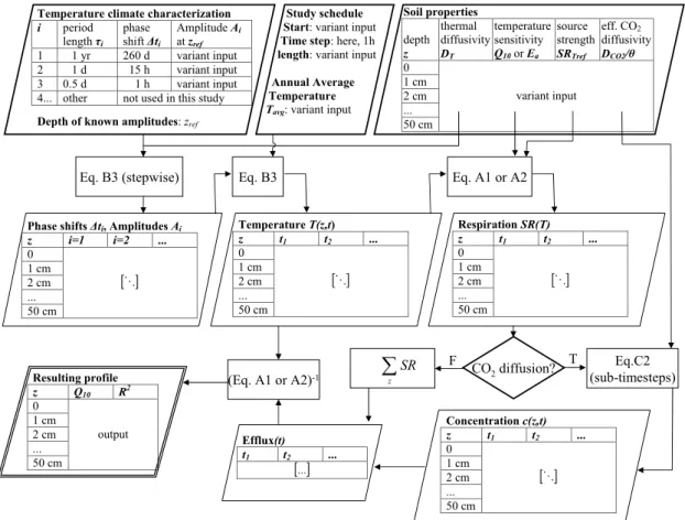
2.2 Model

The model is based on the concept of thermal diffusion and is implemented in For-tran95. An overview of the model architecture is given in Fig.1and the theory behind

25

(6)

tem-BGD

Printer-friendly Version Interactive Discussion perature time series is generated using several distinct sine waves. The annual and

diurnal cycle have a phase shift to correctly reproduce times of maxima and minima, assuming that t=0 is new year’s midnight. A further cycle with a period of 12 h, a phase shift of 1 h, and an amplitudeA=Adiurnal/4 was used to mimic the skewness of

the daily temperature cycle due to slow cooling during the night. Variations of the

diur-5

nal amplitude and day length were not considered. The average temperature was set to the global average (15◦C) in the numerical experiments, and equalled the average measured temperature (12.7◦C) in the model validation. Input amplitudes are deter-mined for the uppermost temperature sensor (0.5 cm) in the model validation. In the numerical experiments, amplitudes were provided for a reference depth of 5 cm. The

10

reason is that amplitudes in this depth are more similar to air temperature than the soil surface temperature. Air temperature amplitudes are globally available and provide a more common reference than surface temperature.

The generated near-surface temperature time series is transferred to other soil depths using an analytical solution of the thermal diffusion equation. This solution

15

does not consider time-variant thermal diffusivity. Instead, we use an effective thermal diffusivity representing the time averaged effect of soil moisture at each depth. On the other hand, time average effective thermal diffusivity may vary strongly with depth due to differences in soil properties and water content. To account for this, the analytic solution was applied in discrete depth steps of 1 cm, using the amplitudes and phase

20

shifts in each layer to calculate those of the next deeper layer (Fig.1). The model is run with a time step of 1 h. Soil respiration is calculated from temperature using the Q10 concept and, as an alternative, also using the Arrhenius concept (see Appendix

A). The source strength of respiration at the average temperature is also given as a depth-dependent value. Here, only a relative vertical distribution is required because

25

absolute values have no effect on the resulting apparent Q10profile.

If CO₂diffusion time from each depth to the soil surface is assumed to be insignifi-cant, the efflux can simply be calculated by integration of the respiration over all depths. However, in analogy to the impact of thermal diffusion on the apparent Q10 discussed

(7)

BGD

Printer-friendly Version Interactive Discussion above, slow gas diffusion could also affect the apparent Q10. To test this

hypothe-sis, we also included CO₂ diffusion in several model runs. As already proposed for heat diffusion, we use an effective diffusivity DCO₂θ

−1

a (Appendix) invariant in time but

vertically distributed. Because the concentration profiles are a result of the vertical source distribution and the nonlinear temperature dependence, CO₂ diffusion cannot

5

be solved analytically. Therefore, we implemented a numerical solution (Appendix). The CO2 flux between two adjacent layers is now the product of diffusivity and the

concentration gradient. We assume no vertical exchange between the lowest layer and the underground. At the surface, a constant atmospheric CO2 concentration of

16.5×103µmol m−3 is maintained. The model considering diffusion requires

initializa-10

tion of the concentration profile. Therefore, the model uses a spin-up period. The length of the spin-up period is considered adequate when the difference in cumulative efflux between runs with and without diffusion is less than 1%.

Finally, the modelled time series of efflux at the surface and temperature in each depth are used to simulate the current practice of field-basedQ10 determination. For

15

each depth, regression of log-transformed efflux against temperature T is used to com-puteQ10. To also test fitting of the Arrhenius relation, the inverse of the temperature is

plotted against the respiration. In this case, the resulting activation energy is converted into aQ10 at the study’s average temperature for comparison (cf.Sanderman et al.,

2003).

20

2.3 Field measurements

An automated soil CO₂flux chamber system (Li-8100, Li-Cor Inc., Lincoln, Nebraska, USA) was operated with four type T thermocouple thermometers at the FLOWatch project test site Selhausen of the Forschungszentrum J ¨ulich. The test site is located in the river Rur catchment (50◦52′09′′N, 06◦27′01′′E, 104.5 m above sea level). The

25

soil is an Orthic Luvisol and the texture is silt loam according to the USDA classifi-cation. A detailed description of the test site is given byWeiherm ¨uller et al. (2007b).

(8)

BGD

Printer-friendly Version Interactive Discussion Organic carbon content was determined in vertical steps of 15 cm. In September 2006,

the soil was tilled up to a depth of 15 cm and power harrowed. Bare field conditions were maintained by a repetition of this treatment in April 2007, several applications of glyphosate, and manual weed control at the efflux measurement plot. Historically, the field was annually ploughed to a depth of 30 cm, and the crop rotation was sugar beet

5

–winter wheat. From 15 October 2006 to 24 April 2007 only one CO2 flux system was

used (closing interval every 30 min). From 24 April to 14 October 2007, four identical chambers with a separation of 20 cm were operated with the Li8100 multiplexer system (closing interval 15 min for each chamber). The soil flux chambers were placed on soil collars of 20 cm in diameter and a height of 7 cm, which were inserted 5 cm into the

10

soil. The system was closed for two minutes for each flux measurement. CO₂and wa-ter vapour concentration as well as chamber headspace temperature were measured every second, and the CO2concentration was corrected for changes in air density and

water vapour dilution. The soil respiration was calculated by fitting a linear regression to the corrected CO2concentrations from 30 s after closing until reopening.

15

The thermocouples used to measure soil temperature have 1 mm thick unshielded joints to ensure a quick response, and were installed horizontally at 0.5, 3, 5, and 10 cm depth, 20 cm away from the chamber system. Temperature data were logged every second while the chamber was closed, and averaged. To vertically extend the empirical apparent Q10 profiles, we also use temperature data of pF-meters (Ecotech, Bonn,

20

Germany) in 15, 30, 45, 60, 90 and 120 cm depth, which were logged independently in 1 h intervals.

To obtain a uniform dataset, the efflux and temperature measurements were reduced to median hourly CO2flux and average hourly soil temperature at each measurement

depth. In the case of CO2 flux, the median was used because it is less sensitive

25

to outliers and non-normal distributions. In the final data set, only those hours were considered where all flux and temperature measurements were available. Because more than 50% of the hours in December and January could not be considered due to power supply problems, these two months were completely excluded from the dataset.

(9)

BGD

Printer-friendly Version Interactive Discussion To determine the effective soil thermal diffusivity, we derived the annual amplitude

in each depth from average daily temperature, and applied the phase equation (e.g.,

Verhoef et al., 1996) to each pair of successive temperature measurement depths. Linear regression providedD_T values for each depth increment.

3 Results

5

3.1 Literature and own field measurements

Figure2shows apparentQ10values as a function of depth from this and other studies.

An increase of apparentQ10 with depth can be seen in all studies, but with a strongly

variable slope. The highest apparent value (Gaumont-Guay et al.,2006,Q10=150 in a

temperature measurement depth of 50 cm) is not shown for scaling reasons. This

pro-10

file is based on measurements taken during two winter months. The second highest value was found byKhomik et al. (2006), also at 50 cm, in long-term measurements excluding winter months, but including snow cover situations in spring, and capturing the diurnal cycle in summer (Table 1). Of the remaining profiles, our own measure-ments and those by Shi et al. (2006), both from farmland and capturing the diurnal

15

cycle, increase strongest with depth. The remaining profiles exhibit comparatively low, but still substantial apparent Q10 increases with depth. In the study by Perrin et al.

(2004), the air temperature 9 m above ground level is included and yields a consider-ably lower value than the three soil temperature series, which are close to each other both in measurement depth and in apparentQ10.

20

The values from studies using a single temperature measurement depth also show Q10values increasing with depth.

3.2 Model validation

Figure 2 also shows the best model fit (RMSE of 0.16) obtained by fitting a depth invariant inputQ10, while assuming a model domain of 50 cm, a homogeneous carbon

(10)

BGD

Printer-friendly Version Interactive Discussion source distribution within the plough layer (0 to 30 cm depth) and a carbon-free subsoil

and neglecting CO₂ diffusion. The depth-invariant input Q10 yielding this optimum fit

was 5.9. We did not consider depth-dependent values of the input Q10 in order to

avoid over-fitting. It should be noted that the results were not substantially different when using an Arrhenius relationship instead of the Q10 concept (not shown). This

5

also applies to all results shown below.

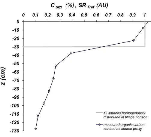
The model fit was less good when using the measured, linearly interpolated Corg

profile (Fig. 3) as a proxy of the source strength distribution. Increasing the length of the model domain to 120 cm also decreased model quality (Table2). The optimal input Q10 values found for these different conditions vary from 5.3 to 6.2, and would

10

have been directly measured in depths between 10 cm and 20 cm. Considering CO₂ diffusion either led to negligible differences or higher errors, depending on diffusivity (also see next sections).

3.3 Numerical experiments

The validated model was used to study the effect of several factors on the apparent

15

Q10 profile. Figure 4 shows apparent Q10 values as a function of both temperature

measurement depth and each factor considered in this study. The depth where theR2 between soil respiration and temperature is highest is indicated withRmax2 . The input

Q10used to generate all plots is 2.5.

In the case of a homogenous respiring A-horizon of varying thickness above a

non-20

respiring subsoil (Fig. 4a), the input Q10 is obtained at about half the depth of the

respiring layer. The highestR2, however, is found at a shallower depth. The difference between the optimal measurement depth and the depth with the highest correlation in-creases with the thickness of the respiring layer (up to 10 cm for a 50 cm thick respiring layer). The apparentQ10at the depth of highestR

2

, however, does not differ more than

25

5% from the input value. Typical measurement depths used in field studies (0 to 10 cm) result in errors ranging from −30 to +10 % depending on the depth of the respiring

(11)

BGD

Printer-friendly Version Interactive Discussion layer. The apparentQ10 values shown in Fig.4a vary from less than 1.8 to more than

3, which is about the range of most reported values (Raich and Schlesinger, 1992), although the inputQ10 was constant at 2.5. In all other plots (Fig.4b to f), we assumed

a respiring layer thickness of 30 cm.

The impact of the length of the measurement period is illustrated in Fig. 4b. For

5

short periods (less than about 180 days), the apparentQ10 behaves highly irregular.

For measurement periods longer than a year, the apparentQ10 is stable throughout

the first 20 cm depth. It should be noted that we assumed that inter-annual variations in average temperature can be neglected here. All other plots are based on a 1 year measurement period.

10

Changing the thermal diffusivity of the soil (one value for all depths, Fig.4c), yields an irregular behaviour for values less than 0.1 mm2s−1. Above this threshold, possi-ble apparent Q10 errors, as well as the distance between the Q10 obtained from the

highestR2and the inputQ10, decreases with increasing diffusivity. We used a thermal

diffusivity of 0.5 mm2s−1in all other plots.

15

The influence of CO₂ transport is neglected in all simulations except for those pre-sented in Fig.4d. Considering gas diffusion leads to an offset in apparent Q10in the first

20 cm compared to cases where diffusion is not considered, but the extent of this offset is less than 2% for effective diffusivities greater than 0.5 mm2s−1. Below 0.5 mm2s−1, this offset increases sharply and the depth of the highest R2can be found below rather

20

than above the depth regaining the inputQ10.

In Fig. 4e, the annual temperature amplitude was varied from 0 to 20 K (twice the value used in the other model runs). For annual amplitudes below the diurnal am-plitude of 5 K, the resulting profile is highly irregular with a local maximum. In addi-tion, the temperature sensitivity is underestimated throughout most of the modelling

25

domain. Figure4f shows the effect of varying diurnal amplitudes. High diurnal ampli-tudes increase the errors made within the first 20 cm, and lead to an underestimation of temperature sensitivity when using shallow temperature sensors. Zero diurnal tem-perature amplitudes yield an almost linear apparentQ10 profile and a close proximity

(12)

BGD

Printer-friendly Version Interactive Discussion of the depth with the highestR2and the input Q10. Note that in our numerical

exper-iments, this behaviour could be reproduced using daily averages of temperature and CO₂efflux. Averaging efflux before or after log-transformation only resulted in negligi-ble differences (∆Q10<0.01). Simulating only one measurement per day at a fixed time

also yields similar results, but with a small vertical offset of about 3 cm depending on

5

the time of day of the measurement.

4 Discussion

4.1 Literature and own field measurements

The variability of theQ10 dependence on temperature measurement depth underlines

the need for a methodology that allows comparison of temperature sensitivities

de-10

termined in field experiments. Various explanations for the variability of apparentQ10

profiles can be deduced from our modelling exercise. The highest reported appar-entQ10 (Gaumont-Guay et al.,2006) is based on those authors’ deepest temperature

measurements and a short study period of two months. The amplitude of the diurnal temperature is strongly attenuated at that depth, and the amplitude of the annual

cy-15

cle is not fully sampled because of the short measurement period. Therefore, CO2

efflux was correlated to temperature values with small amplitude and high phase shift, which can result in very high or very low apparentQ10 values. The second highestQ10

increase with depth (Khomik et al., 2006) originates from a study capturing the daily temperature cycle in summer, with additional less frequent measurements in spring

20

and autumn, and no measurements in winter. The steep profiles found by Shi et al.

(2006) and by ourselves were obtained for agricultural soils without temperature atten-uation effects on the diurnal cycle by abundant vegetation. The lowest increase of Q10

with depth was found in a study where measurements of the diurnal cycle of CO2efflux

were avoided (Wang et al.,2006). The air temperature in proximity to the forest canopy

25

(13)

BGD

Printer-friendly Version Interactive Discussion forest soil temperatures and consequently yields a lower apparentQ10.

Vegetation does not only affect the temperature regime of the soil, but also respi-ration itself. All studies discussed here except for our own bare soil measurements include both heterotrophic and root respiration. Hanson et al. (2000) review various studies on the contribution of root to total soil respiration. Depending on ecosystem,

5

they find that 10 to 90% of total respiration stems from roots with an average contribu-tion of about 50%. Root respiracontribu-tion is related not only to those environmental variables that are known to influence heterotrophic respiration, but also to aboveground plant productivity and thus to radiation (Tang et al.,2005). This correlation is subject to a lag between several hours and several days (Moyano et al.,2008), due to the time taken

10

by phloem transport from leaves to roots. The similarity between this lagged response to radiation and soil temperature at a certain depth, which may also be considered a lagged response to radiation, could cause confusion. In the interpretation of mixed soil respiration, too much of temporal variability might be attributed to either soil tempera-ture or aboveground radiation, depending on normalisation procedure and the available

15

temperature measurement depth. In general, however, we may expect the presence of another controlling factor to weaken the depth dependence of the apparentQ10. This

would be in good agreement with the fact that dense and high forest sites generally seem to yield somewhat more stable profiles in Fig.2, as would the damping effect of the canopy on the temperature regime.

20

4.2 Model validation

The model application to the field data demonstrates that the model is able to describe the temperature sensitivity variation with depth. The remaining uncertainty of about ±10% occurs when considering deeper layers, and their carbon content (Table2). We attribute this to two main causes. First, temperature measurement errors become

in-25

creasingly significant deeper in the soil, where amplitudes are smaller. Such errors are not simulated by the model. However, temperature sensitivity of soil respiration is rarely determined from temperature sensors installed in large depths. Second, there is

(14)

BGD

Printer-friendly Version Interactive Discussion considerable uncertainty in the source strength distribution. Organic carbon content

in-cludes accumulated stable carbon pools, the fraction of which can be depth-dependent itself. The field data were best described when neglecting the organic carbon content found below the A-horizon. This seems to indicate that deeper carbon is less involved in respiration activity, which is in good agreement with the general assumption that

5

carbon pools in deeper horizons are more stable (cf.Fierer et al.,2003). The increas-ing uncertainty with depth also implies that field measurements of CO₂ efflux at the soil surface are not suited to derive the temperature sensitivity of deep buried carbon, which has been associated with higher temperature sensitivities by some (Knorr et al.,

2005;Davidson and Janssens,2006). Our study shows that although a true increase

10

ofQ10 with depth may be present, it should not be confused with the temperature

mea-surement depth dependence of the apparentQ10.

It was not necessary to consider CO2diffusion to model the apparent Q10 variation

with depth for our field experiment. This fits well with the results of the numerical experiments discussed in the next section, which showed that for most diffusivities

15

observed in the field the impact should be low (Fig.4d;Tang et al.,2003;Werner et al.,

2004). Nevertheless, a general recommendation to neglect CO₂ transport should not be made based on the results of a single field study.

It is noteworthy that the measurement depths that would have yielded a Q10 value

in the range of the optimal input Q10 of the model, are below 10 cm, while all single

20

measurement depths found in our literature study are above that depth. At least in the case of this site, relying on literature conventions would thus have likely underestimated temperature sensitivity.

Finally, it should be mentioned that the model only considers the pure confounding factor temperature measurement depth. Depending on the site characteristics, other

25

confounding effects, such as correlation of temperature with moisture (Davidson et al.,

1998), may cause errors of similar magnitude in field-basedQ10 determination. In the

frequent case of negative correlation between temperature and moisture, the result will again be an underestimation of temperature sensitivity.

(15)

BGD

Printer-friendly Version Interactive Discussion 4.3 Numerical experiments

When the vertical source strength distribution consists of a homogenous respiring layer above a non-respiring sub-soil, the best depth to place a single temperature sensor is the centre of the respiring layer (Fig.4a). Although such a distribution is not unrealistic for our field reference dataset, it may be not fulfilled in non-agricultural soils, especially

5

in the presence of litter layers. As an alternative method to determine the most appro-priate depth,Tang et al. (2003), Perrin et al. (2004) and Shi et al. (2006) suggested the maximumR2 criterion. Although our numerical experiments show that this is not exactly correct, it is a good approximation in most conditions. However, both the R2 criterion and the centre placement fail in extreme conditions, as illustrated in Fig.4b to

10

e.

The difference between the depth of highest R2 and the depth regaining the input Q10 is a result of the combined effect of amplitude attenuation and phase shift of

tem-perature waves. For an infinitely thin respiring layer, theR2is highest for a temperature measurement within this layer. This measurement will also provide the correct Q10.

15

At other depths, the R2 is lower due to phase shifts in the temperature time series. For thicker respiring layers, efflux at the surface integrates over CO2 production time

series with different delays and amplitudes. If the delay is considered in isolation, the highestR2 would occur in the middle the respiring layer. However, the apparent Q10

would underestimate the temperature sensitivity for all depths because the averaging

20

of several phase-shifted temperature waves results in a smaller range of temperature values. When amplitude attenuation and phase shifts are both considered, deeper parts of the respiring layer show a smaller variance in both, temperature and their con-tribution to column respiration. Therefore, the depth of highestR2 is shifted upwards. At the same time, the lower temperature amplitudes in these depths counteract the

25

underestimation of the apparentQ10. Strictly spoken, the temperature measurement

depth regaining the inputQ10 is not a “correct” depth, but a depth where positive and

(16)

BGD

Printer-friendly Version Interactive Discussion The depth that regains the inputQ10 will not always be within the respiring layer, as

illustrated by Fig.4b. In this figure, the length of the measurement period was varied. The model qualitatively confirms that extremely high apparent temperature sensitivities for greater measurement depths, such as those found byGaumont-Guay et al.(2006) andKhomik et al. (2006), can be caused by incomplete representation of the annual

5

cycle. For a more quantitative assessment, too little is known especially on the varying thickness and thermal properties of the snow cover, which was an important feature in both studies. The fact that measurement periods of less than half a year can result in highQ10 errors is also relevant to studies separating the study period into seasons

to capture plant phenological effects on temperature sensitivity (e.g.,Xu and Qi,2001;

10

Yuste et al.,2004;deForest et al.,2006).

Variation of the soil thermal diffusivity (Fig.4c) confirms the expectation that accurate field-based Q10 measurements are more likely when temperature waves propagate

rapidly into the ground. According to Zmarsly et al. (2002), most soils have thermal diffusivities ranging between 0.1 (dry organic) and 0.75 mm2s−1(wet sand). Therefore,

15

the irregular behaviour of the apparent Q10 for very low diffusivities is not relevant in

most ecosystems.

Effective CO2 diffusivities can cover a much larger range. A compilation of Werner

et al. (2004) based on 81 studies shows that DCO₂θ −1

a can range from 0.09 to more

than 12 mm2s−1. Despite this large range, our numerical experiment shows that the

20

influence of diffusion on apparent Q10 would be negligible for all but the three lowest

values summarized byWerner et al.(2004). It is interesting that for such small diffu-sivities, the depth of highestR2can drop below the depth regaining the inputQ10. We

attribute this to the fact that the time series of surface efflux is now delayed compared to the temperature time series in those depths where most of the CO₂ is produced.

25

Consequently, efflux correlates better with deeper temperature time series. This is no indication of a causal relationship, as the CO2 produced in these depths is delayed

even stronger before reaching the surface.

(17)

BGD

Printer-friendly Version Interactive Discussion avoid systematic errors when temperature sensitivities from different climatic zones

are compared. Close to the equator where the annual amplitude is low, field-based determination of accurateQ10 values is difficult. Typically, the temperature sensitivity

will be underestimated. Continental and boreal climates with high annual amplitudes potentially allow an accurate determination of theQ10 when the measurement period

5

is long and continuous. This may be difficult in case of harsh winter conditions, or be complicated by the thermal properties of a snow cover (see above).

The numerical experiment on diurnal amplitude (Fig.4f) is of particular interest be-cause the positive effects of low diurnal amplitudes can be approximated by daily av-eraging of efflux and temperature time series. A similar reduction in daily amplitude

10

can be obtained by measurements at a fixed time of day, but it remains to be exam-ined whether this alternative is more susceptible to varying day lengths and amplitudes throughout the year.

5 Conclusions

We described the development, validation, and application of a simple model to explain

15

and estimate the errors in temperature sensitivity determination related to the temper-ature measurement depth. We chose the widely usedQ10concept as an example, but

the alternative activation energy concept provides almost identical results.

Depending on study conditions, the vertical profile of the apparent Q10 may range

from fairly regular to highly irregular. The latter case can include local minima and

20

maxima, decoupling of the depth of correct Q10 from the depth of highest R 2

, and cases where the obtained Q10 is incorrect for all conventional temperature

measure-ment depths. In these cases, only laboratory incubation experimeasure-ments directly can yield correct temperature sensitivity relations, although these experiments are not free of errors and assumptions either. An alternative possibility would be to inversely estimate

25

theQ10 using numerical models of CO2 production, CO2 transport and heat transport

(18)

BGD

Printer-friendly Version Interactive Discussion properties and CO₂ source strength (Herbst et al.,2008;Novak,2007;Weiherm ¨uller

et al.,2007a) and could be extended toQ10estimation.

In many field studies, however, the detailed input data required to drive mechanistic CO₂ models are not available. In such cases, the model presented here, and some basic climate and soil data, may help reducing errors in temperature sensitivity

anal-5

ysis. However, validation has shown that an uncertainty remains due to the choice of input parameters. Also, analyses of additional field data sets to test whether the sim-plifications made within the model are justified would be desirable. Nevertheless, the model clearly helps recognizing field study conditions whereQ10determination is fairly

reliable. The following conditions allow an accurate estimation ofQ₁₀:

10

– a thin and easily distinguished horizon of respiration activity,

– a measurement period of one year or more,

– a high thermal and CO2diffusivity of the soil,

– a high annual temperature amplitude,

– daily averaging of measurements before fitting the temperature sensitivity

func-15

tion.

Our analyses indicate that a temperature measurement depth within the upper 10 cm, as is commonly used in field studies, is likely to result in an underestimation of temperature sensitivity, at least in the absence of a litter layer. According to the lat-est IPCC report (Solomon et al.,2007), most models used to estimate the biochemical

20

feedback of land surfaces to climate change assume a soil respirationQ10 close to 2.

It is noteworthy that this assumption is based on averaging not only laboratory but also field studies (Solomon et al., 2007), e.g. those compiled by Raich and Schlesinger (1992). These models predict a global effective sensitivity of heterotrophic respiration of 6.2% per K warming. However, a largerQ10 of 2.5 would be well within the

uncer-25

(19)

BGD

Printer-friendly Version Interactive Discussion third in each model, which is the same order of magnitude as the standard deviation

among the models. The models give an average absolute sensitivity of land surfaces to climate change of −79 Gt sequestered carbon per K warming, although this rate is highly variable between the models (±45 GtC K−1). An additional uncertainty of one third due to an unknown primary temperature sensitivity of respiration, divided by the

5

time span over which such a 1 K increase is assumed to occur (40 to 50 years depend-ing on scenario), would be equal to 7 to 9% of the current annual emissions from fossil fuel burning and cement production.

Appendix A

10

Temperature sensitivity functions

Two methods are most commonly used to relate temperature and respiration. The first is an empirical exponential relationship suggested by van t’Hoff (e.g.,Yuste et al.,

2004): SR = SRT_refe

lnQ10

10 (T −Tref) _(A1)

15

whereSR is soil respiration (µmol m−2s−1),T is temperature (K) and Tref is an

arbi-trary reference temperature with a know respiration rateSRT_ref. Q10is the rate by which

respiration changes with a temperature change of 10 K. TheQ10 is a commonly used

parameter to report the temperature sensitivity of soil respiration. The second relation-ship is more physically based and uses activation energy considerations introduced by

20

Arrhenius (e.g.,Lloyd and Taylor,1994):

SR = SRT_refe

Ea

R T Tref(T −Tref)

(A2) Here,E_ais the activation energy (J mol−1), andR=8.314 J mol−1K−1is the universal gas constant. Further temperature sensitivity functions are summarised byK ¨atterer et

(20)

BGD

Printer-friendly Version Interactive Discussion al. (1998) and Bauer et al. (2008). The temperature sensitivity coefficients of these

methods (Q10 and Ea) are not equivalent. For typical temperature and respiration

ranges, aQ10value derived from Eq. (A2) based onEadecreases slowly with

increas-ing temperature, whereas Q10 is a constant in Eq. (A1). A slow Q10 decrease with

increasing temperature has been reported in a range of field and laboratory studies

5

(e.g., Kirschbaum,2006;Shi et al., 2006). Large differences between both relations only occur in the case of extrapolation, especially into warmer conditions. However, it has been questioned whether extrapolation can be used for future feedback prediction (Davidson and Janssens,2006). One reason for this is that different soil carbon pools may have different temperature sensitivities. A long-term temperature change would

10

then change the pool ratios and, consequently, the effective temperature sensitivity of the soil. It is still under debate whether these effects are of a measurable and relevant magnitude or not (Fang et al.,2005;Knorr et al.,2005;Reichstein et al.,2005;Conen

et al.,2006;Larinova et al.,2007).

Appendix B

15

Theory of soil temperature profiles

Soil surface temperature changes are mainly induced by the radiation balance at the soil surface and exchange of sensible and latent heat between the soil and the atmo-sphere. The variation in soil surface temperature propagates into deeper layers. In the

20

absence of transport of sensible and latent heat in the soil gas phase (Weber et al.,

2007), this process is controlled by the soil thermal diffusivity DT (m2s−1):

∂T ∂t = DT ∂2T ∂z2 = λ ρc ∂2T ∂z2 (B1)

wheret is time (s) and z is depth (m). Thermal diffusivity is a function of thermal conductivityλ (W m−1K−1), heat capacityc (J kg−1K−1), and bulk densityρ (kg m−3).

(21)

BGD

Printer-friendly Version Interactive Discussion The typical order of magnitude of soil thermal diffusivity is 10−7to 10−6m2s−1(Zmarsly

et al.,2002). To transfer a soil temperature time series to another depth, it is often rep-resented by a series of sine waves (de Vries,1963;Verhoef et al.,1996;Heusinkveld

et al.,2004;Graf et al.,2008):

T = T + n X i =1 A_isin2π(t + ∆ti) τi (B2) 5

whereT denotes the average temperature (K), Ai is the temperature amplitude (K),

τ_i is the period length (s), and ∆ti the phase shift (here in units of time and therefore

included in the bracketed term) of the sine wave indexedi . When thermal diffusivity is constant with depth and time, there is an analytical solution to Eqs. (B1) and (B2) (de Vries,1963) that predicts temperature in any other depth (Heusinkveld et al.,2004;

10 Graf et al.,2008): T = T + n X i =1 A_iexp ∆z s π DTτi ! sin 2_{π(t + ∆t}_i ₊∆zτi 2π q π D_Tτ_i) τ_i (B3)

where ∆z is the difference between the actual and the reference depth. Stepwise application of Eq. (B3) allows to treat thermal diffusivities that change along a vertical profile (cf. methods section).

(22)

BGD

Appendix C

Theory of gas diffusion

Diffusion of CO2through soil air is described by:

∂c

∂t = τθaDa ∂2ca

∂z2 + SR (C1)

5

wherec is the total volumetric concentration of CO2,ca is the concentration in soil

air,Dais the diffusivity of CO2in air (m 2

s−1),θa(dimensionless) is the soil air content,

andτ is a dimensionless tortuosity factor. Da, the soil air content, tortuosity and other

factors such as transport through soil water and pressure turbulence can be combined into an effective diffusivity (Simunek and Suarez, 1993; Hirano et al., 2003; Tang et

10

al.,2003;Takle et al., 2004). In this study, we use a wide range of field-determined effective diffusivities reviewed byWerner et al.(2004). To solve Eq. (C1), we use an explicit time discretization:

c(t + ∆t, z) = c(t, z) + ∆t(SR(t, z) +DCO₂(z − 12∆z) c(t,z−∆z)−c(t,z) θa∆z2 −D_CO 2(z + 1 2∆z) c(t,z)−c(t,z+∆z) θa∆z2 ) (C2) 15

By definingDCO₂ in planes 0.5 ∆z above and below all other depth-dependent input

data, we achieve mass-consistency. The maximum value of the time-step for a stable solution is ∆t<0.5∆z2D−1_CO

2θa.

Acknowledgements. Field assistance by Rainer Harms and partial funding of A. Graf’s

post-doctoral appointment by the “Impuls- und Vernetzungsfonds” of the Helmholtz Association are

20

gratefully acknowledged. Equipment is financed by the Helmholtz-funded FLOWatch project and the DFG-funded Transregional Collaborative Research Centre SFB TR 32 “Patterns in Soil-Vegetation-Atmosphere Systems: Monitoring, Modelling, and Data Assimilation”.

(23)

BGD

References

Bauer, J., Herbst, M., Huisman, J. A., Weiherm ¨uller, L., and Vereecken, H.: Sensitivity of sim-ulated soil heterotrophic respiration to temperature and moisture reduction functions, Geo-derma, GEODER-09851, doi:10.1016/j.geoderma.2008.01.026, in press, 2008. 1885

Borken, W., Davidson, E. A., Savage, K., Gaudinski, J., and Trumbore, S. E.: Drying and

5

wetting effects on carbon dioxide release from organic horizons, Soil Sci. Soc. Am. J., 67, 1888–1896, 2003. 1870

Chen, X. Y., Eamus, D., and Hutley, L. B.: Seasonal patterns of soil carbon dioxide efflux from a wet-dry tropical savanna of northern Australia, Aust. J. Bot., 50, 43–51, 2002.1870

Conen, F., Leifeld, J., Seth, B., and Alewell, C.: Warming mineralises young and old carbon

10

equally, Biogeosciences, 3, 515–519, 2006,

http://www.biogeosciences.net/3/515/2006/. 1885

Davidson, E. A. and Janssens, I. A.: Temperature sensitivity of soil carbon decomposition and feedbacks to climate change, Nature, 440, 165–173, 2006.1869,1879,1885

Davidson, E. A., Belk, E., and Boone, R. D.: Soil water content and temperature as

indepen-15

dent or confounded factors controlling soil respiration in a temperate mixed hardwood forest, Global Change Biol., 4, 217–227, 1998.1869,1870,1879

deForest, J. L., Noormets, A., McNulty, S. G., Sun, G., Tenney, G., and Chen, J.: Phenophases alter the soil respiration-temperature relationship in an oak-dominated forest, Int. J. Biome-teorol., 51, 135–144, 2006.1870,1881

20

de Vries, D. A.: Thermal properties of soils, in: Physics of Plant Environment, edited by: van Wijk, W. R., North-Holland, Amsterdam, The Netherlands, 210–233, 1963. 1886

Dugas, W. A.: Micrometeorological and Chamber Measurements of CO₂Flux from Bare Soil, Agr. Forest Meteorol., 67, 115–128, 1993. 1870

Fang, C., Moncrieff, J. B., Gholz, H. L., and Clark, K. L.: Soil CO2efflux and its spatial variation

25

in a Florida slash pine plantation, Plant Soil, 205, 135–146, 1998. 1870

Fang, C. M., Smith, P., Moncrieff, J. B., and Smith, J. U.: Similar response of labile and resistant soil organic matter pools to changes in temperature, Nature, 433, 57–59, 2005. 1885

Fierer, N., Allen, A. S., Schimel, J. P., and Holden, P.: Controls on microbial CO₂production: a comparison of surface and subsurface horizons, Global Change Biol., 9, 1322–1332, 2003.

30

1879

(24)

Inter-BGD

preting the dependence of soil respiration on soil temperature and water content in a boreal aspen stand, Agr. Forest Meteorol., 140, 220–235, 2006. 1869,1874,1877,1881

Graf, A., Kuttler, W., and Werner, J.: Mulching as means to exploit dewfall for arid agriculture?, Atmos. Res., 87, 369–376, 2008. 1886

Hanson, P. J., Edwards, N. T., Garten, C. T., and Andrews, J. A.: Separating root and soil

micro-5

bial contributions to soil respiration: A review of methods and observations, Biogeochemistry 48, 115–146, 2000.1878

Hashimoto, S. and Komatsu, H.: Relationships between soil CO₂concentration and CO₂ pro-duction, temperature, water content, and gas diffusivity: implications for field studies through sensitivity analyses, J. Forest Res. –JPN, 11, 41–50, 2006. 1869

10

Herbst, M., Hellebrand, H. J., Bauer, J., Huisman, J. A., Simunek, J., Weiherm ¨uller, L., Graf, A., Vanderborght, J., and Vereecken, H.: Multiyear heterotrophic soil respira-tion: evaluation of a coupled CO₂ transport and carbon turnover model, Ecol. Model., doi:10.1016/j.ecolmodel.2008.02.007, in press, 2008. 1883

Heusinkveld, B. G., Jacobs, A. F. G., Holtslag, A. A. M., and Berkowicz, S. M.: Surface energy

15

balance closure in an arid region. Role of soil heat flux, Agr. Forest Meteorol., 122, 21–37, 2004. 1886

Hirano, T., Kim, H., and Tanaka, Y.: Long-term half-hourly measurement of soil CO₂ concentra-tion and soil respiraconcentra-tion in a temperate deciduous forest, J. Geophys. Res. Atmos., 108(D20), 4631, doi:10.1029/2003JD003766, 2003. 1869,1887

20

Humphreys, E. R., Black, T. A., Morgenstern, K., Cai, T. B., Drewitt, G. B., Nesi, Z., and Trofy-mow, J. A.: Carbon dioxide fluxes in coastal Douglas-fir stands at different stages of devel-opment after clearcut harvesting, Agr. Forest Meteorol., 140, 6–22, 2006. 1870

K ¨atterer, T., Reichstein, M., Andr ´en, O., and Lomander, A.: Temperature dependence of organic matter decomposition: a critical review using literature data analyzed with different models,

25

Biol. Fert. Soils, 27, 258–262, 1998. 1884

Khomik, M., Arain, M. A., and McCaughey, J. H.: Temporal and spatial variability of soil respi-ration in a boreal mixedwood forest, Agr. Forest Meteorol., 140, 244–256, 2006.1869,1874,

1877,1881

Kim, J. and Verma, S. B.: Soil CO₂flux in a Minnesota peatland, Biogeochemistry, 18, 37–51,

30

1992. 1870

Kirschbaum, M. U. F.: The temperature dependence of organic-matter decomposition – still a topic of debate, Soil Biol. Biochem., 38, 2510–2518, 2006. 1885

(25)

BGD

Knorr, W., Prentice, I. C., House, J. I., and Holland, E. A.: Long-term sensitivity of soil carbon turnover to warming, Nature, 433, 298–301, 2005. 1879,1885

Larinova, A. A., Yevdokimov, I. V., and Bykhovets, S. S.: Temperature response of soil respi-ration is dependent on concentrespi-ration of readily decomposable C, Biogeosciences, 4, 1073– 1081, 2007,

5

Law, B. E., Falge, E., Gu, L., et al.: Environmental controls over carbon dioxide and water vapor exchange of terrestrial vegetation, Agr. Forest Meteorol., 113, 97–120, 2002.1870

Lloyd, J. and Taylor, J. A. On the temperature-dependence of soil respiration, Funct. Ecol., 8, 315–323, 1994. 1869,1884

10

Lou, Y. S., Li, Z. P., and Zhang, T. L.: Soil CO₂flux in relation to dissolved organic carbon, soil temperature and moisture in a subtropical arable soil of China, J. Environ. Sci.-China, 15, 715–720, 2003. 1870

Moyano, F. E., Kutsch, W. L., and Rebmann, C.: Soil respiration fluxes in relation to pho-tosynthetic activity in broad-leaf and needle-leaf forest stands, Agr. Forest Meteorol., 148,

15

135–143, 2008. 1870,1878

Novak, M. D.: Determination of soil carbon dioxide source-density profiles by inversion from soil-profile gas concentrations and surface flux density for diffusion-dominated transport, Agr. Forest Meteorol., 146, 189–204, 2007.1883

Novick, K. A., Stoy, P. C., Katul, G. G., Ellsworth, D. S., Siqueira, M. B. S., Juang, J., and Oren,

20

R.: Carbon dioxide and water vapor exchange in a warm temperate grassland, Oecologia, 138, 259–274, 2004. 1870

Perrin, D., Laitat, E., Yernaux, M., and Aubinet, M.: Modelling the response of forest soil respi-ration fluxes to the main climatic variables, Biotechnol. Agron. Soc. Environ., 8, 15–25, 2004.

1869,1874,1877,1880

25

Raich, J. W. and Schlesinger, W. H.: The global carbon dioxide flux in soil respiration and its relationship to vegetation and climate, Tellus, 44(B), 81–99, 1992.

Reichstein, M., K ¨atterer, T., Andr `en, O., Ciais, P., Schulze, E. D., Cramer, W., Papale, D., and Valentini, R.: Temperature sensitivity of decomposition in relation to soil organic matter pools: critique and outlook, Biogeosciences, 2, 317–321, 2005,

30

Sanderman, J., Amundson, R. G., and Baldocchi, D. D.: Application of eddy covariance mea-surements to the temperature dependence of soil organic matter mean residence time,

(26)

BGD

Global Biogeochem. Cy., 17, 1061, doi:10.1029/2001GB001833, 2003. 1872

Savage, K. E. and Davidson, E. A.: A comparison of manual and automated systems for soil CO₂ flux measurements: trade-offs between spatial and temporal resolution, J. Exp. Bot., 54, 891–899, 2003.1870

Shi, P. L., Zhang, X. Z., Zhong, Z. M., and Ouyang, H.: Diurnal and seasonal variability of

5

soil CO₂efflux in a cropland ecosystem on the Tibetan Plateau, Agr. Forest Meteorol., 137, 220–233, 2006. 1869,1874,1877,1880,1885

Simunek, J. and Suarez, D. L.: Modeling of carbon-dioxide transport and production in soil. 1. Model development, Water Resour. Res., 29, 487–497, 1993.1887

Solomon, S., Qin, D., Manning, M., et al. (Eds.): Climate Change 2007: The Physical Science

10

Basis, Contribution of Working Group I to the Fourth Assessment Report of the Intergovern-mental Panel on Climate Change Cambridge University Press, Cambridge, United Kingdom and New York, NY, USA, 501–539, 2007. 1883

Takahashi, A., Hiyama, T., Takahashi, H. A., and Fukushima, Y.: Analytical estimation of the vertical distribution of CO₂production within soil: application to a Japanese temperate forest,

15

Agr. Forest Meteorol., 126, 223–235, 2004. 1870

Takle, E. S., Massmann, W. J., Brandle, J. R., et al.: Influence of high-frequency ambient pressure pumping on carbon dioxide efflux from soil, Agr. Forest Meteorol., 124, 193–206, 2004. 1887

Tang, J. W., Baldocchi, D. D., Qi, Y., and Xu, L. K.: Assessing soil CO₂efflux using continuous

20

measurements of CO₂profiles in soils with small solid-state sensors, Agr. Forest Meteorol., 118, 207–220, 2003. 1869,1879,1880,1887

Tang, J. W., Baldocchi, D., and Xu, L. K.: Tree photosynthesis modulates soil respiration on a diurnal time scale, Global Change Biol., 11, 1298–1304, 2005. 1878

Tang, J., Bolstad, P. V., Desai, A. R., Martin, J. G., Cook, B. D., Davis, K. J., and Carey, E. V.:

25

Ecosystem respiration and its components in an old-growth forest in the Great lakes region of the United States, Agr. Forest Meteorol., 148, 171–185, 2008.1870

Verhoef, A., van den Hurk, B. J. J. M., Jacobs, A. F. G., and Heusinkveld, B. G.: Thermal soil properties for vineyard (EFEDA-I) and savanna (HAPEX-Sahel) sites, Agr. Forest Meteorol., 78, 1–18, 1996. 1874,1886

30

Wang, C., Yang, J., and Zhang, Q.: Soil respiration in six temperate forests in China, Global Change Biol., 12, 2103–2114, 2006. 1869,1877

(27)

BGD

coarse substrates –Field measurements versus a laboratory test, Theor. Appl. Climatol., 89, 109–114, 2007. 1885

Weiherm ¨uller, L., Huisman, J. A., Graf, A., Herbst, M., and Vereecken, H.: Multistep outflow experiments for the simultaneous determination of soil physical and CO₂production param-eters, EGU General Assembly, Vienna, Austria, 16–20 April 2007, EGU07-A-01742, 2007a.

5

1883

Weiherm ¨uller, L., Huisman, J. A., Lambot, S., Herbst, M., and Vereecken, H.: Mapping the spatial variation of soil water content at the field scale with different ground penetrating radar techniques, J. Hydrol., 340, 205–216, 2007b. 1872

Werner, D., Grathwohl, P., and H ¨ohener, P.: Review of field methods for the determination

10

of the tortuosity and effective gas-phase diffusivity in the vadose zone, Vadose Zone J., 3, 1240–1248, 2004. 1879,1881,1887

Xu, M. and Qi, Y.: Spatial and seasonal variations ofQ10determined by soil respiration mea-surements at a Sierra Nevada forest, Global Biogeochem. Cy., 15, 687–696, 2001. 1869,

1881

15

Yuste, J. C., Janssens, I. A., Carrara, A., and Ceulemans, R.: Interactive effects of temperature and precipitation on soil respiration in a temperate maritime forest, Tree Physiol., 23, 1263– 1270, 2003. 1870

Yuste, J. C., Janssens, I. A., Carrara, A., and Ceulemans, R.: Annual Q(10) of soil respiration reflects plant phenological patterns as well as temperature sensitivity, Global Change Biol.,

20

10, 161–169, 2004.1881,1884

Zmarsly, E., Kuttler, W., and Pethe, H.: Meteorologisch-klimatologisches Grundwissen, Ulmer, Stuttgart, Germany, 2002. 1881,1886

(28)

BGD

Table 1. Studies providing multiple Q10 values due to multiple temperature measurement

depths.

reference method site frequency period

1 Xu and Qi (2001) chamber ponderosa pine plantation, ≥1 month−1, Jun 1998–Aug 1999

Sierra Nevada, USAa ≥6 day−1

2 Hirano et al. (2003) profile temperate deciduous forest, 2 h−1 May 2000–Nov 2000

Japan

3 Tang et al. (2003) profile oak-grass savannah, 2 h−1 Jul 2002–Nov 2002

Sierra Nevada, USA

4 Perrin et al. (2004) chamber beech forest, 2 h−1 Jun 2000–Jul 2003

Ardennes, Belgium

5 Gaumont-Guay et al. (2006) chamber boreal aspen forest, 2 h−1 Jan 2001–Feb 2001

central Canada

6 Khomik et al. (2006) chamber boreal forest, 1 month−1 b, Jul 2003–Jul 2005

eastern Canada not in winter

7 Shi et al. (2006) chamber irrigated farmland, ≥1 month−1, Sep 1999–Aug 2001

Tibetan Plateau ≥2 day−1 c

8 Wang et al. (2006) chamber six different forests, 2 week−1 Apr 2004–Oct 2005

north-eastern China a

results given separately for two sites b

moring and afternoon of the measurement day in summer, once per day in transition months c

(29)

BGD

Table 2.Results of model validation under different settings.

source domain optimal RMSE

profile depth inputQ10

1 (>−30 cm), 0 (<−30 cm) 50 cm 5.9 0.16 1 (>−30 cm), 0 (<−30 cm) 120 cm 5.3 0.80 measured C_org 50 cm 6.2 0.21 measured C_org 120 cm 5.9 1.20

(30)

BGD

Printer-friendly Version Interactive Discussion t i A i z i = 1 i = 2 [ ] (t) t 1 t 2 [ ] T( z , t z t 1 t 2 [ ] S R( T) z t 1 t 2 [ ] z D T Q 1 0 E a ! S R T r e f "# D C O 2 /θ " $% "# &

∑

( ' c ( z , t) z t 1 t 2 [ ] z Q 1 0 R 2 % ) ) * ) T a vg ) i ! τ i ✫t i A i z r e f + , ! " # )

Fig. 1. Overview of the model architecture. Bold outline: Input parameters; doubled outline:

(31)

BGD

Fig. 2. Empirical apparentQ₁₀as a function of temperature measurement depth z. Numbers

refer to the study bibliography given in Table2, single depth references are listed in the methods section. Depths>0 denote air temperature (height not to scale).

(32)

BGD

(33)

BGD

Printer-friendly Version Interactive Discussion ! "# $ % & ' () $ % * + +* +% , -+ & % +* ( .( ( ( "# / + 0 &$ 1 +* $ ( 2 % $ 2$ 3 ( 2++ 2 % $ 2 3 ( θ & , & + 4 + & $ % + & *

Fig. 4. ApparentQ₁₀resulting from simulated hourly flux measurements as a function of

tem-perature measurement depthz and: (a) thickness of a homogenous respiring layer, (b)

mea-surement period, (c) thermal diffusivity (one for all depths), (d) effective CO2 diffusivity, (e) annual temperature amplitude, (f) diurnal temperature amplitude.DCO2 is infinite in all but (d).