HAL Id: hal-00298047
https://hal.archives-ouvertes.fr/hal-00298047
Submitted on 17 Jul 2006
HAL is a multi-disciplinary open access
archive for the deposit and dissemination of
sci-entific research documents, whether they are
pub-lished or not. The documents may come from
teaching and research institutions in France or
abroad, or from public or private research centers.
L’archive ouverte pluridisciplinaire HAL, est
destinée au dépôt et à la diffusion de documents
scientifiques de niveau recherche, publiés ou non,
émanant des établissements d’enseignement et de
recherche français ou étrangers, des laboratoires
publics ou privés.
W. F. Ruddiman
To cite this version:
W. F. Ruddiman. Ice-driven CO2 feedback on ice volume. Climate of the Past, European Geosciences
Union (EGU), 2006, 2 (1), pp.43-55. �hal-00298047�
www.clim-past.net/2/43/2006/
© Author(s) 2006. This work is licensed under a Creative Commons License.
Climate
of the Past
Ice-driven CO
2
feedback on ice volume
W. F. Ruddiman
Department of Environmental Sciences, University of Virginia, Charlottesville, VA, USA Received: 17 January 2006 – Published in Clim. Past Discuss.: 15 February 2006 Revised: 8 June 2006 – Accepted: 3 July 2006 – Published: 17 July 2006
Abstract. The origin of the major ice-sheet variations
dur-ing the last 2.7 million years is a long-standdur-ing mystery. Neither the dominant 41 000-year cycles in δ18O/ice-volume during the late Pliocene and early Pleistocene nor the late-Pleistocene oscillations near 100 000 years is a linear (“Mi-lankovitch”) response to summer insolation forcing. Both responses must result from non-linear behavior within the climate system. Greenhouse gases (primarily CO2) are a
plausible source of the required non-linearity, but confusion has persisted over whether the gases force ice volume or are a positive feedback. During the last several hundred thou-sand years, CO2 and ice volume (marine δ18O) have
var-ied in phase at the 41 000-year obliquity cycle and nearly in phase within the ∼100 000-year band. This timing rules out greenhouse-gas forcing of a very slow ice response and instead favors ice control of a fast CO2response.
In the schematic model proposed here, ice sheets re-sponded linearly to insolation forcing at the precession and obliquity cycles prior to 0.9 million years ago, but CO2
feed-back amplified the ice response at the 41 000-year period by a factor of approximately two. After 0.9 million years ago, with slow polar cooling, ablation weakened. CO2feedback
continued to amplify ice-sheet growth every 41 000 years, but weaker ablation permitted some ice to survive insolation maxima of low intensity. Step-wise growth of these longer-lived ice sheets continued until peaks in northern summer insolation produced abrupt deglaciations every ∼85 000 to
∼115 000 years. Most of the deglacial ice melting resulted from the same CO2/temperature feedback that had built the
ice sheets. Several processes have the northern geographic origin, as well as the requisite orbital tempo and phasing, to be candidate mechanisms for ice-sheet control of CO2 and
their own feedback.
Correspondence to: W. F. Ruddiman ([email protected])
1 Introduction
Milankovitch (1941) proposed that orbitally controlled changes in summer insolation at high northern latitudes drive ice-volume responses at the 23 000-year period of preces-sion and the 41 000-year period of tilt. Using marine δ18O as an ice-volume proxy, Hays et al. (1976) confirmed that ice sheets fluctuate at those periods and also verified Mi-lankovitch’s prediction that the responses lag several thou-sand years behind orbital forcing (Fig. 1a). Fluctuations at non-orbital periods are not addressed here.
Milankovitch did not anticipate two features found in ma-rine δ18O records. One is the strength of the 41 000-year cycle in δ18O and other climate proxies prior to 900 000 years ago (Muller and MacDonald, 2000; Raymo and Ni-sancioglu, 2003). This dominance is inconsistent with the Milankovitch hypothesis because summer insolation varia-tions at high northern latitudes are considerably stronger at the period of precession than at the period of tilt. The second unexpected feature is the strong δ18O (ice-volume) oscilla-tion centered on a period near 100 000 years during the late Pleistocene (Shackleton and Opdyke, 1976). The small ef-fect of orbital eccentricity on incident solar radiation rules out insolation as the direct cause of these longer-wavelength changes in ice volume.
Milankovitch’s insolation hypothesis thus provides a valid starting point for an orbital theory of climate, but not a full explanation. As a result, many scientists have explored the next most important orbital-scale variable in the climate sys-tem – changes in concentration of carbon dioxide (CO2)and methane (CH4). At this point, however, widely divergent views coexist about the effect of greenhouse gases (partic-ularly CO2)on ice sheets. Two end-member views are
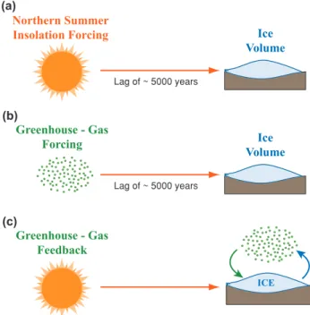
Northern Summer
Insolation Forcing Ice
Volume Lag of ~ 5000 years Greenhouse - Gas Forcing Greenhouse - Gas Feedback Ice Volume Lag of ~ 5000 years (a) (c) (b) ICE Fig. 1
Fig. 1. (a) Northern hemisphere summer insolation forces ice sheets
with lags of several thousand years (Milankovitch, 1941; Hays et al., 1976). Greenhouse gases could either force ice sheets with the same lag (b), or be driven by ice-sheet variations and provide posi-tive feedback to the ice (c).
One possibility is that CO2forces ice volume (Pisias and
Shackleton, 1986; Genthon et al., 1987; Imbrie et al., 1992, 1993; Shackleton, 2000). In this view, changes in CO2
“push” the slow-responding ice sheets, which respond with lags of 5000 years or more (Fig. 1b). These lags are anal-ogous to the ice-volume response to changes in insolation (Fig. 1a).
An alternative possibility is that CO2 concentrations are
controlled by ice volume and act as a fast positive feedback on ice-sheet mass balance (Ruddiman, 2003; see also Clark et al., 1999). In this case, little or no lag should exist be-tween changes in CO2and in ice volume (Fig. 1c). Each
in-crement of ice growth (whether over a millennium or a cen-tury) causes greenhouse-gas concentrations to fall, and the reduced gas levels immediately promote further ice growth during that same millennium or century. Once the ice sheets begin to shrink, the greenhouse gas levels rise, promoting further ice melting.
Because both ice sheets and CO2concentrations are parts
of the overall response of a highly coupled climate system with complex feedbacks, progress in understanding cause and effect at orbital scales has been difficult. The problem, once summarized by Laurent Labeyrie, is that “Everything is correlated to everything”.
One potential clue to the cause-and-effect problem is the relative phasing of the greenhouse gases and ice volume. Do the gas changes precede ice volume and thus force a slow ice
CO
2CO
2 3300 yrs 4300 yrs CO2 CH4 3000 yrs 3400 yrs ~ 6500 yrs ~ 4500 yrs Forcing Feedback Tilt Precession Tilt Precession (a) SPECMAP (1992) (b) Ruddiman (2003) CO2 CH4 ICE ICE ICE ICE Fig. 2Fig. 2. Phase relationships among insolation, greenhouse gases,
and ice-volume at the periods of orbital precession and tilt. (a) SPECMAP (Imbrie et al., 1992) inferred that CO2forces ice vol-ume as part of a chain of responses to orbital insolation. (b) Tuning of gas records in Vostok ice (Ruddiman and Raymo, 2003; Shack-leton, 2000) indicates that CO2and CH4combine with insolation to force ice volume at 23 000 years, but act as ice-driven feedbacks at 41 000 years.
response (Fig. 1b)? Or do they respond in phase with the ice and thus act as a “fast feedback” (Fig. 1c)?
2 CO2and ice volume at the obliquity and precession
cycles
The SPECMAP group (Imbrie et al., 1992, 1993) presented a comprehensive hypothesis on the role of greenhouse gases in orbital climatic change. At a time when Vostok drilling had not recovered enough ice to constrain the timing of long-term CO2 variations, SPECMAP attempted to use geochemical
proxies for this purpose. At the periods of orbital precession and tilt, SPECMAP proposed that changes in summer insola-tion at high northern latitudes initiate a complex chain of re-sponses that are transferred south via deep-water flow. Sub-sequent changes in the south-polar region then produce CO2
variations that ultimately drive the slow-responding northern ice sheets (Fig. 2a) [SPECMAP did not consider the role of methane.].
Once the actual CO2 record preserved in Vostok ice air
(2000) created a gas time by tuning the precession compo-nent of δ18Oairto an insolation target signal with a
Septem-ber phase. Subsequently, Ruddiman and Raymo (2003) de-veloped an independent gas time scale by tuning the preces-sion component of the CH4signal to an insolation target with
mid-July (summer monsoon) phasing. These two time scales yielded average phases for the obliquity and precession com-ponents of the CO2variations that agreed to within less than
100 years (see also Bender, 2002).
At the 23 000-year precession period, both CH4and CO2
have phases on or close to that of northern mid-summer in-solation (Fig. 2b). For methane, this timing is supported by the match between the CH4 peak 10 500 years ago in
annually layered Greenland ice (Blunier et al., 1995) and the age of the most recent July insolation maximum. It is also consistent with mid-summer (July) forcing of monsoon maxima that create methane-generating wetlands in southern Asia (Kutzbach, 1981; Prell and Kutzbach, 1992; Yuan et al., 2004). The phase of CO2at the 23 000-year period falls
less than 1000 years after that of July insolation. These early phases for both methane and CO2indicate that the two
green-house gases (along with summer insolation) act as sources of forcing of ice volume at the 23 000-year period (Ruddiman, 2003).
In contrast, both methane and CO2 vary in phase with δ18O/ice volume at the 41 000-year period of obliquity (Fig. 2b). This in-phase behavior rules out greenhouse-gas forcing of a slow (lagged) ice response. Instead, the ice sheets must drive fast gas responses with little or no lag. These ice-driven gas variations then provide positive feed-back to both the growth and melting of ice sheets at 41 000 years. The reason for the different behavior of CO2and CH4
at the precession and obliquity cycles is beyond the scope of this paper.
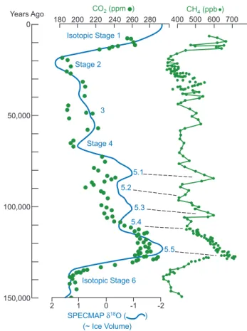
For the most recent glacial-interglacial oscillation, δ18O changes (Fig. 3) are linked to changes in ice volume by sea-level constraints from coral reefs (Chappell and Shackleton, 1986; Bard et al., 1990). Sea level can be converted to ice volume and to changes in δ18O by assuming 10 m of change per 0.11‰ of δ18O shift (Fairbanks and Mathews, 1978). By this measure, ice volume accounts for well over half of the
δ18O change on the major δ18O transitions: 50–70% of ter-minations II (the stage 6/5 δ18O boundary) and I (the stage 2/1 boundary); 50–60% of the substage 5.5/5.4 δ18O transi-tion; 100% of the substage 5.4/5.3 boundary, ∼70% of the stage 5/4 transition, and ∼65% of the stage 3/2 boundary.
The δ18O trends in Fig. 3 are consistent with the results from spectral analysis. The maxima at marine isotopic stages 4 and 2 are manifestations of the 41 000-year cycle. Both occur several thousand years after insolation minima at the obliquity cycle, consistent with a forced (and lagged) ice-volume response (Imbrie et al., 1992). The coincident CO2
minima at these times indicate that CO2acted as an in-phase
feedback at the obliquity cycle, amplifying the size of these ice-volume maxima without altering their phase.
180 200 220 240 260 280 400 500 600 700 CO2 (ppm ) CH4 (ppb ) 5.4 5.5 5.3 5.2 5.1 Stage 4 3 Stage 2 2 1 0 -1 -2 Isotopic Stage 6 Isotopic Stage 1 SPECMAP δ18O ( ) Years Ago 0 50,000 100,000 150,000 Fig. 3 (~ Ice Volume)
Fig. 3. Comparison of normalized SPECMAP δ18O record (Imbrie et al., 1984) against Vostok CO2and CH4signals according to the GT4 time scale of Petit et al. (1999). The SPECMAP time scale is shifted to older ages by 2000 years.
In contrast, evidence of greenhouse-gas forcing of ice volume is present during isotopic stage 5, when insolation changes at the 23 000-year precession cycle were largest. At that time, large methane variations (of ∼250 ppb) clearly led δ18O by several thousand years, indicating that methane changes forced a lagged ice-volume response. Hints of a sim-ilar lead appear near isotopic substages 5.5 and 5.1 in the noisier, lower-resolution CO2signal.
Because the 41 000-year signal is roughly twice as strong as that at 23 000 years in the signals of both CO2 (Petit et
al., 1999) and δ18O (Imbrie et al., 1984, 1992), the feedback role for CO2outweighs the ice-forcing role in the combined
effects of these two periods.
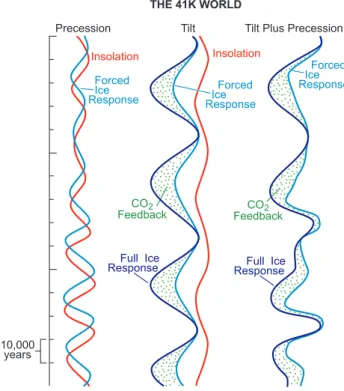
3 Conceptual model: 41 000-year cycles of ice volume from 2.7 to 0.9 million years ago
The above observations can be applied to the early regime of Northern Hemisphere glaciation. Near 2.75 million years ago, north polar latitudes cooled to the point that reduced summer insolation periodically allowed moderately large ice
CO2
Feedback FeedbackCO2
Insolation Insolation
Precession Tilt Tilt Plus Precession
Forced Ice Response Forced Ice Response Forced Ice Response Full Ice
Response Full IceResponse
10,000 years
THE 41K WORLD
Fig. 4
Fig. 4. Schematic model of CO2 feedback on ice volume in the 41 K world prior to 0.9 million years ago. Summer insolation at 65◦N forces ice volume at the precession cycle. Summer insolation forcing of ice volume at the tilt cycle is 40% of that at the precession cycle. The greater length of the tilt cycle increases the forced ice response compared to that at precession. Positive CO2 feedback amplified the 41 000-year ice response so that the combined ice-volume signal was dominated by tilt. (Insolation trends shown are those of the last 150 000 years).
sheets to form, but all or most of the ice melted during each subsequent interval of increased insolation. For nearly the first two million years of the northern hemisphere ice ages,
δ18O variations were dominated by 41 000-year variations (Pisias and Moore, 1981; Ruddiman et al., 1986; Raymo et al., 1989), despite the fact that changes in summer insola-tion forcing were stronger at the 23 000-year precession cy-cle, both on a monthly basis and for the entire caloric summer half-year.
This mismatch between forcing and response is reduced to some extent by the fact that ice volume has almost twice as long to respond to forcing at the 41 000-year cycle as it does at the 23 000-year cycle because of the greater interval over which the forcing persists (41 000/23 000=1.8. For an e-folding ice response, the ratio would be somewhat smaller,
∼1.5. Even with allowance for this longer time of integration of the effect of tilt forcing, the average ice-volume response at the precession period still exceeds that at obliquity by al-most 50%.
One way to resolve the remaining mismatch between the summer insolation forcing and the observed δ18O responses
20˚ 15˚ 10˚ G lo ba l m ea n te m pe ra tu re ( ˚C ) 1000 800 600 200 0 400 Interglacial Glacial
Atmospheric CO2 concentration (ppm)
Fig. 5
Fig. 5. Logarithmic relationship between CO2concentration and global temperature for the model examined by Oglesby and Saltz-man (1990).
is to suppress the 23 000-year precession component of the
δ18O signal by interhemispheric cancellation of oppositely phased ice responses between the northern and southern hemispheres (Raymo et al., 2006). Another proposed reso-lution is the fact that the large amplitude of precession peaks is offset by changes in length of the summer season (P. Huy-bers, personal communication, 2006).
The suggestion has also been made that insolation changes at the obliquity cycle enhanced the planetary temperature gradient and drove a greater northward flux of tropical mois-ture (Young and Bradley, 1984; Raymo and Nisancioglu, 2003; Vettoretti and Peltier, 2004). Glacial geologists and glaciologists, however, generally view accumulation as a far weaker factor in ice-sheet mass balance than ablation (Al-ley, 2003; Denton et al., 2005). Most simulations with gen-eral circulation models show reduced precipitation in regions where ice accumulates because local cooling reduces the amount of water vapor in the atmosphere.
The explanation favored here is greenhouse-gas feedback at the 41 000-year period. If greenhouse-gas changes at this cycle acted as a positive feedback (as they have done for the last 400 000 years; Fig. 2b), they would have amplified the 41 000-year ice-volume response to direct insolation forcing and caused additional (non-linear) ice growth at that cycle. In the example shown in Fig. 4, the direct ice-volume response to insolation forcing at the 41 000-year cycle is arbitrarily as-sumed to have doubled in size because of positive CO2
feed-back. This proposed doubling would make the 41 000-year ice-volume signal the dominant orbital response.
CO2 CO2 ICE 100K Phases 15,000 10,000 5,000 E 5,000 10,000 15,000 Years after E Years before E Eccentricity CO2 CO2 CH4 ICE ICE ~ 12,000 yrs ~ 15,000 yrs SPECMAP (1993) Shackleton (2002) Ruddiman (2003) (ITF) Ice-Driven Ice-Driven Ice-Driven Fig. 6
Fig. 6. Phase relationship between CO2 and ice volume in the ∼100 000-year band. SPECMAP (Imbrie et al., 1993) inferred that CO2 forces ice volume as part of a chain of responses to orbital insolation. Shackleton (2000) also inferred CO2forcing of ice vol-ume, but with the entire process offset ∼10 000 years later in time. Ruddiman (2003) inferred that CO2is primarily a fast feedback on ice volume, based on the similar phasing of CO2and δ18O. Phases of “ice-driven responses” (North Atlantic sea-surface temperature, dust, deep-water circulation) are indicated.
The effect of CO2 on global temperature is weakly
log-arithmic: the change in global temperature per unit change of CO2 increases with lower concentrations (Fig. 5). As a
result, the positive temperature feedback on ice volume aris-ing from changes in CO2at the 41 000-year cycle would also
have been weakly logarithmic.
Although the level of dominance in the conceptual ex-ample shown in Fig. 4 does not match that in marine ben-thic δ18O records, the isotopic signals are overprinted by a large (and apparently in-phase) temperature response at the 41 000-year cycle (Raymo et al., 1989). That overprint ex-aggerates the strength of the 41 000-year signal in benthic
δ18O records compared to actual changes in ice volume, and the amount of amplification is not precisely known. The schematic example shown may thus be in reasonable accord with the real behavior of ice sheets.
In this schematic model of the 41 000-year regime, the combined insolation forcing at the precession and tilt cycles accounts for about 70% of the amplitude of the orbital-band ice-volume response, while CO2feedback provides the other
30%. Even though CO2 feedback is critical to explaining
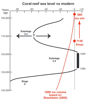
the unexpected prominence of the 41 000-year signal in this earlier climatic regime, forced responses still dominated ice-sheet behavior. ? Substage 5.4 Substage 5.5 Stage 6 +10 0 -20 -40 -60 -80 100,000 110,000 120,000 130,000 140,000 128K 120K
Coral-reef sea level vs modern
Years ago 98K Ice min 113K Emax 100K ice volume based on Shackleton (2000) Fig. 7
Fig. 7. Estimated sea-level changes during marine isotopic
sub-stages 5.5 and 5.4 from coral reefs and δ18O signals (Chappell and Shackleton, 1986; Bard et al., 1990) compared with filtered 100 000-year ice-volume signal based on Shackleton (2000).
4 Relative phasing of CO2 and ice volume in the ∼100 000-year eccentricity band
4.1 Spectral analysis
Late Pleistocene climatic records of many kinds have been dominated by oscillations in a band centered on 100 000 years, especially during the last 400 000 years. SPECMAP (Imbrie et al., 1993) proposed that CO2changes in this band
occurred as an intermediate step within a chain of responses (Fig. 6). The initial driver of the CO2 signal was referred
to as an (unidentified) “internal thermal forcing” or ITF. The CO2response arose within the climate system when ice
sheets began to exceed a certain size threshold and produce other feedbacks. But once again the direct role proposed for CO2in the SPECMAP scheme was to force ice sheets, which
in this case responded with a much longer lag of ∼12 000 years.
Shackleton (2000) later determined that the ∼100 000-year CO2signal in Vostok ice has a much later phase than
Imbrie et al. (1993) had inferred from geochemical proxies, one on or very close to the phase of eccentricity. He sug-gested that the 100 000-year CO2signal arose from processes
operating within the carbon system independently of the ice sheets. Shackleton further proposed that the 100 000-year marine δ18O signal in benthic foraminifera carries a very
large temperature overprint and that the actual 100 000-year phase of ice volume is offset some 12 000 years later than the
δ18O signal. This revised interpretation maintained CO2as
the immediate source of forcing of ice volume (Fig. 6), but it shifted the entire forcing-and-response relationship ∼10 000 years later in time compared to the scheme of Imbrie et al. (1993).
Ruddiman (2003) concluded that the extremely late phase inferred by Shackleton (2000) for the 100 000-year compo-nent of ice volume is not consistent with other evidence. For example, it would mean that an ice-volume minimum at the 100 000-year period should have occurred 98 000 years ago, 15 000 years after the preceding eccentricity maximum (Fig. 7). This timing implicitly requires that ice was gradu-ally melting at the ∼100 000-year period through the entire first half of marine isotopic stage 5. But oxygen-isotopic and coral-reef evidence indicate that renewed ice growth during marine isotopic substage 5.4 culminated in an ice-sheet max-imum of substantial size near 110 000 years ago (Imbrie et al., 1984; Chappell and Shackleton, 1986). This scenario is highly implausible: if large ice sheets were rapidly growing during substage 5.4 in the only known centers of northern hemisphere glaciation, how could “100 000-year” ice sheets have been slowly melting at this same time elsewhere on Earth?
A second problem with such a late ice-volume response is that it lags thousands of years behind a group of northern responses widely regarded as “ice-driven”: North Atlantic sea-surface temperatures, northern hemisphere dust fluxes, and NADW flow (Ruddiman and McIntyre, 1984; Raymo et al., 1989; Imbrie et al., 1993). If these signals were driven by the ice sheets, they could not have led their “drivers” by
∼10 000 years. Based on these criticisms, Ruddiman (2003) concluded that δ18O is a good first-order proxy for ice vol-ume during the large climatic oscillations of the late Pleis-tocene, in agreement with the traditional view of CLIMAP (Hays et al., 1976) and SPECMAP (Imbrie et al., 1984), and many other studies over several decades.
If δ18O is a valid proxy for ice volume, the phase lag be-tween CO2and ice volume (δ18O) at the 100 000-year cycle
cannot be more than a few thousand years. In the absence of significant insolation forcing at this period, eccentricity is used here a convenient reference point for comparing the phases of CO2and δ18O. The SPECMAP group (Imbrie et
al., 1984, 1989) estimated that the δ18O signal lags eccentric-ity by ∼3300 years, but subsequent U-series dating of coral reefs and sea level (Edwards et al, 1987; Bard et al., 1990) led to revisions of this estimate. Several studies concluded that the SPECMAP time scale is on average too young by 1500 to 2000 years (Pisias et al., 1990; Shackleton, 2000; Ruddiman, 2003). If the phase of the δ18O signal at the ∼100 000-year period is adjusted by 2000 years, its lag behind eccentricity would be only ∼1300 years. As for the CO2signal, tuned
Vostok time scales indicate that it could either be in phase with eccentricity (Shackleton, 2000) or lead it by as much as
3500 years (Ruddiman and Raymo, 2003; Ruddiman, 2003). Consequently, the overall CO2lead versus δ18O (ice volume)
in the ∼100 000-year band would be ∼1300 to ∼4800 years (Fig. 6).
4.2 Cross-correlation analysis
Fourier analysis is not an optimal way to assess leads and lags between CO2and δ18O in the ∼100 000-year band. Both
signals have highly asymmetric shapes that drift gradually to-ward “glacial” values (low CO2and positive δ18O) and then
shift abruptly to “interglacial” conditions (high CO2and
neg-ative δ18O) across deglacial transitions. A symmetrical sine wave with a period near 100 000 years cannot capture either the abruptness of the terminations or the fundamental saw tooth asymmetry of the major glacial/interglacial cycles near
∼100 000 years (Muller and MacDonald, 2000).
An alternative approach is to compare the relative tim-ing of the full CO2 and ice-volume signals. Using
cross-correlation analysis, Mudelsee (2001) found that the CO2
signal at Vostok (Petit et al., 1999) lagged SPECMAP δ18O by 3700±2800 years between 420 000 and 200 000 years ago, but led it by 3200±4000 years since that time. Compar-ison with a benthic δ18O record from the Indian Ocean indi-cated a CO2lead of 2700±1300 years over the last 420 000
years. Comparison to the δ18Oairrecord at Vostok indicated
a CO2lead of 3900±500 years.
This analysis shows that CO2 and δ18O are in phase to
within a few thousand years, with a general tendency toward a small CO2 lead. Because both the CO2 and δ18O signals
are dominated by power in the ∼100 000-year band, this re-sult further confirms the conclusion that the phase separation between CO2and ice volume at that period is small.
4.3 Leads and lags on terminations
Several studies have focused on the relative timing of CO2
and ice-volume changes across deglacial terminations. Dur-ing termination I, CO2 changes lead coral-reef (sea-level)
indices of ice volume by 1000 years or less (Broecker and Henderson, 1998; Alley et al., 2002). The estimated CO2
lead relative to δ18O on termination II was ∼3000 years (Broecker and Henderson, 1998), but sizeable uncertainties exist in both the dating of both signals and in the accuracy of the ice-volume proxies (Alley et al., 2002).
In summary, three methods of comparing the timing of changes in CO2and δ18O (ice volume) converge on a small
CO2lead in the range of 1000 to 4000 years, with
uncertain-ties of a few thousand years.
5 CO2/ice phasing at ∼100 000 years: CO2 forcing or
feedback?
Spectral analysis, cross-correlation analysis, and analysis of leads and lags on terminations all rule out the possibility that
CO2 leads ice volume by 12 000 years at the 100 000-year
period, as proposed by Imbrie et al. (1993) and Shackle-ton (2000). That conclusion also eliminates the interpreta-tion that CO2 forces ice sheets with a large time constant
of ∼15 000 years at this period. The observed phasing be-tween CO2and δ18O leaves open two interpretations: either
(1) CO2forces fast-responding ice sheets that lag by only a
few thousand years, or (2) CO2is in phase with ice volume
and acts as a positive feedback.
In order for CO2 to lead and force ice sheets in the
100 000-year band, the ice response time would have to be very rapid. The response time of ice sheets at a given pe-riod can be calculated from the phase lag of δ18O behind CO2from the arctangent relationship of Imbrie et al. (1984): 8=arctan 2πf T . where 8 is the phase lag of the ice sheets (in degrees out of 360◦)relative to the forcing, f is the fre-quency of the forcing in years (here, 1/100 000), and T is the ice time constant in years. For a phase lag of 1000–4000 years at the 100 000-year period, the time constant required for the ice sheets would lie in the same range (1000–4100 years).
Such a small time constant does not seem unreasonable for the rapid disintegration of marine portions of ice sheets that calve icebergs to the ocean, but it is far more problematic for the bulk of the ice in continental interiors. The strongest evidence against so short an ice response is the lag of 5000 to 8000 years of marine δ18O signals behind summer insolation at the forced cycles of 23 000 and 41 000 years. These lags formed the quantitative basis for the SPECMAP marine time scale and they require ice-sheet response times of at least 5000 years (Imbrie et al., 1993), longer than the values of 1000 to 4100 years calculated above.
The other plausible interpretation is that CO2acts
primar-ily as an ice-driven feedback that has the same phase as the ice, or very nearly so. Given the large uncertainties in most of the above estimates, this interpretation is permitted by the very small phase difference between CO2 and δ18O in the
band near ∼100 000 years.
The interpretation favored here is that the phasing of CO2
and ice volume in the ∼10 000-year band is the result of both feedback and forcing processes, but that the in-phase feed-back contribution is the larger of the two. This conclusion is consistent with the strong in-phase CO2feedback at the
41 000-year period and the weaker CO2forcing at the 23
000-year period during the last 400 000 000-years (Fig. 2b). 5.1 CO2feedback at the last glacial maximum
The evidence summarized above suggests a prominent feed-back role for CO2in orbital-scale variations. Evidence that
CO2 may in fact be the dominant orbital-scale feedback in
the climate system comes from the last glacial maximum, the only pre-modern interval examined in sufficient regional detail to allow a global-scale assessment of processes that af-fect climate (Hansen et al, 1984; Raynaud et al, 1988; Hoffert
and Covey, 1992). Because summer and winter solar radia-tion values 21 000 years ago were similar to those today, in-solation differences are not regarded as a major explanation of the colder glacial-maximum temperatures. Instead, these studies suggest that the primary feedbacks in operation were greenhouse gases and albedo.
The ∼90-ppm CO2lowering at the last glacial maximum
provided a radiative cooling of ∼0.67◦C, and the ∼320-ppb CH4decrease added another ∼0.14◦C, including the
chemi-cal effects of methane on stratospheric ozone (Raynaud et al, 1988). The combined radiative cooling of ∼0.81◦C would have been amplified by a factor of 2.1 by other factors (pri-marily water vapor) for a 2.5◦C global-mean sensitivity to CO2doubling. The resulting total greenhouse-gas cooling of
1.7◦C would then account for about 40% of the total global cooling of ∼4.5◦C (±0.7◦) at the last glacial maximum.
Albedo-temperature feedback accounts for most of the re-maining glacial-maximum cooling (Hansen et al, 1984; Hof-fert and Covey, 1992). About half of this albedo increase came from the bright surfaces of the northern hemisphere ice sheets, but a substantial part resulted from the increased ex-tent of Southern Ocean sea ice. Because the glacial increase in Antarctic sea ice has been attributed to lower greenhouse-gas levels (Broccoli and Manabe, 1987), this effect should probably be added to the greenhouse-gas side of the ledger, bringing the total gas contribution to more than 50%. In ad-dition, part of the remaining albedo increase came from a re-duction in glacial vegetation cover caused by lower CO2
val-ues, further increasing the indirect greenhouse contribution (Levis and Foley, 1999). Greenhouse gases (mainly CO2)
thus appear to have been the dominant feedback that kept the world cold at the last glacial maximum. The bright high-albedo surfaces of the northern ice sheets accounted for much of the rest of the feedback.
In summary, CO2acts primarily as an in-phase feedback
on ice volume, while CO2 forcing of ice sheets plays a
smaller role. The next two sections summarize a conceptual model of ice-volume oscillations in the 100 000-year band that builds on these conclusions.
6 Conceptual model of ∼100 000-year ice-volume oscil-lations
6.1 Ice growth every 41 000 years
In the schematic model of the 41 K world (Sect. 3), north-ern hemisphere ice sheets grew at intervals of 41 000 years, but then melted entirely during the subsequent insolation maxima. Gradually, however, temperatures were cooling during the late Pliocene and early Pleistocene, causing a slow drift to more positive marine δ18O values (Mix et al., 1995). In the late Pleistocene, variations in ice volume be-came larger in size and longer in wavelength. By 400 000 years ago, sawtooth-shaped δ18O oscillations centered on the
Fig. 8
Insolation Insolation
Forced Ice Response
minimum Insolation maximum maximum Ice Volume minimum Precession
Years Ago Tilt Tilt Plus Precession
THE 100K WORLD CO2 Feedback FeedbackCO2 Full Ice Response Full Ice Response Forced Ice Response Forced Ice Response 0 50,000 100,000 150,000
Fig. 8. Schematic model of CO2 feedback on ice volume in the ∼100 K world since 0.9 million years ago. As in the 41 K world, insolation forced ice volume at the precession and tilt cycles, the greater length of the tilt cycle increased the forced ice response compared to precession, and CO2feedback amplified ice growth every 41 000 years. Following ice-growth episodes, reduced abla-tion in a colder world allowed much of the new ice to survive weak insolation minima, and the ice-volume steps at 41 000-year intervals (green arrows) were transformed into a longer-period (∼100 K) re-sponse.
∼100 000-year band had become dominant. The analysis in this section suggests that one simple change in the climate-system response — a substantial reduction in ice ablation — could account for the growth of larger ice sheets centered in the ∼100 000-year band rather than 41 000-year cycles.
The focus here is again on the most recent ∼100 000-year ice-growth oscillation (Fig. 3), because it is both the best dated and the one with the clearest evidence that δ18O in-creases represent ice volume. In the benthic marine δ18O stack of Lisiecki and Raymo (2005), the net δ18O shift to glacial-maximum values during this interval was achieved in three distinct steps at prominent δ18O boundaries: substage 5.5/5.4 (+1.0‰), stage 5/4 (+0.8‰), and stage 3/2 (+0.7‰). Only at these three times did the δ18O signal (and global ice volume) reach values higher than at any time earlier in this oscillation. In addition, all three δ18O transitions were times when CO2concentrations were falling to prominent minima.
All three of these transitions occurred during times of near-alignment of northern summer insolation minima at the tilt and precession cycles, and thus at times of coincident forcing of ice volume by both cycles. A critical question is whether these new increments of ice growth were related to both in-solation cycles or just to one of them.
Two other precession insolation minima during this inter-val produced small δ18O increases (at the substage 5.3/5.2 boundary and within stage 3), but neither of these increases shifted the δ18O signal to values more positive than those reached previously. This observation suggests that the three ice-growth transitions are critically linked to processes tied to the 41 000-year cycle.
The three shifts toward more positive δ18O values are sim-ilar to those during the earlier 41 K world. In the benthic marine δ18O stack of Lisiecki and Raymo (2006), the av-erage δ18O increase during 41 000-year cycles prior to 0.9 million years ago was 0.7‰ (the range was 0.4–1.1‰). The increases across the three δ18O transitions within the last cli-matic oscillation averaged 0.83‰, or ∼20% larger than the mean for the 41 K world.
The primary difference from the earlier 41 K regime is that δ18O values failed to return to their original levels af-ter each new maximum. The 1.0‰ increase across the sub-stage 5.5/5.4 boundary was followed by a 0.35‰ δ18O de-crease across the substage 5.4/5.3 transition, leaving a net isotopic shift of +0.65‰. The 0.8‰ increase across the stage 5/4 boundary was followed by a 0.3‰ δ18O decrease across the stage 4/3 transition, leaving a net isotopic shift of +0.5‰ (The stage 3/2 increase of 0.6‰ was erased by termination I.).
These observations suggest a simple schematic model of how the larger ice-volume oscillations of the late Pleistocene developed (Fig. 8). Just as in the 41 K world, insolation changes at the periods of precession and tilt drove lagged ice-volume responses (again assumed to be linear). And again, CO2feedback selectively amplified the ice-volume response
at 41 000 years, although now by ∼20% more than the dou-bling assumed for the 41 K world (Fig. 4).
The major difference compared to the 41 K world is that ablation was now much lower during the insolation max-ima that followed ice-growth episodes every 41 000 years. Roughly 65% of the new ice that grew on these major tran-sitions survived and formed a new base level for further growth. These three assumptions (linear insolation forcing, CO2 feedback at 41 000 years, and reduced ablation)
pro-duce a sawtooth-shaped buildup of ice over intervals that last longer than a single 41 000-year cycle (Fig. 8).
Why would ablation have decreased so markedly between the 41K world and the ∼100 K world? The explanation prob-ably lies in the ice mass-balance relationship shown in Fig. 9. Because ice ablation is an exponential function of warm-season temperature, a relatively small polar cooling could have greatly diminished summer ablation. But since ice mass balance in winter is much less sensitive to temperature, polar cooling would have caused little change in net snow accu-mulation. Consequently, in a world with colder north-polar regions, larger ice sheets would have grown in a step-wise fashion primarily because of reduced ablation.
Such a trend toward reduced ablation is implicit in the longer-term history of northern ice sheets. Prior to
2.75 million years ago, strong ablation in a warmer world kept northern ice sheets of significant size from forming even during the most favorable orbital configurations. From 2.75 to 0.9 million years ago, reduced ablation in a cooler world allowed growth of ice sheets every 41 000 years, but the next insolation maximum (whether weak or strong) melted most or all of the ice. After 0.9 million years ago, further cooling and additional reduction in ablation permitted ice sheets to survive weaker insolation maxima and persist for longer intervals. In this progression toward a colder world, the Antarctic ice sheet is the next step: ablation rates there have fallen so low that ice survives even the largest insola-tion maxima.
Non-linear CO2/temperature feedback also helped to
re-duce rates of ablation. The growth of very large (“100 K”) ice sheets presumably drove CO2concentrations lower than
those that had been attained during the earlier 41 K world. The lower CO2values would have further cooled
tempera-tures because of the logarithmic relationship shown in Fig. 5. The cooler temperatures would have further reduced ablation of very large ice sheets. Ice-albedo feedback would also have aided CO2in promoting the growth of larger ice sheets.
In this conceptual model (Fig. 8), the growth of larger ice sheets in the ∼100 K world primarily results from CO2
feed-back. Insolation forcing of a linear (Milankovitch) ice re-sponse accounts for ∼25% of the net increase in ice volume between the marine isotopic substage 5.5 interglaciation and the last glacial maximum at isotopic stage 2. The other 75% of the amplitude of the ice build-up results from the transfor-mation of CO2feedback at the 41 000-year cycle into
asym-metric, saw-tooth oscillations in the ∼100 K band. Unlike the 41 K world, the ∼100 K world was dominated by feed-backs (primarily CO2, but also ice albedo).
6.2 Deglaciation every ∼100 000 years
A major question remains. Why did abrupt deglacial termi-nations occur within a band centered near 100 000 years? The discovery that the ∼100 000-year component of δ18O is phase-locked to eccentricity (Hays et al., 1976) suggested that these deglaciations might be linked in some way to mod-ulation of precession by eccentricity at periods averaging near 100 000 years.
Raymo (1997) noted that the time span between successive terminations tends to fall on or near multiples of the 23 000-year precession period, either after four cycles (∼92 000 years) or five (∼115 000 years). She concluded that the
∼100 000-year “cycle” is actually quantum in nature, rather than periodic, and that it is paced mainly by eccentricity modulation of precession peaks in insolation, with insolation maxima at the tilt cycle playing a lesser role.
In contrast, Huybers and Wunsch (2004) concluded that terminations occur at or near multiples of the 41 000-year tilt cycle: after either two cycles (∼82 000 years) or three (∼123 000 years). One problem with invoking only tilt as
Accumulation Equilibrium Line Ablatio n (a) North South Equilibrium Ice accumulation (b) 1 0 -1 -2
Ice mass balance (m/yr)
Annual surface temperature (˚C)
-30 -20 -10
Ice melting
Fig. 9
Fig. 9. Geographic and climatic constraints on ice-sheet mass
bal-ance. (a) Zonal cross section of northern ice sheets. Equilibrium line separates areas of net accumulation and ablation. (b) Ice mass balance as a function of mean annual temperature. Long-term cool-ing reduces strong warm-season ablation.
the key forcing is that a large amount of ice had accumulated by isotopic stage 4, and a strong 41 000-year insolation max-imum followed in stage 3, but less than half of the ice present at that time melted (∼30 m of sea-level equivalent).
Insolation forcing at the periods of both precession and tilt probably plays a role in determining the timing of termi-nations (Imbrie et al., 1992, 1993). The individual contribu-tions from these two periods were closely aligned at termina-tions I and IV and were offset by only ∼4000 years on termi-nation II. Tilt and precession forcing were not closely aligned during Termination III, and probably as a result, deglaciation at that time was incomplete.
But only a small fraction of the amount of ice melting at terminations can be explained by a linear ice response to in-solation forcing. Most of the melting resulted from feedback processes operating within the climate system (Imbrie et al., 1993).
CO2is the primary internal feedback that maintained cold
temperatures during the glacial maximum (Sect. 5), and CO2was proposed earlier in this section as the key positive
feedback that causes non-linear growth of large ice sheets (Fig. 8). When favorable orbital configurations provided suf-ficient forcing to initiate deglacial melting, this same positive feedback was readily available to amplify ice melting. As the large glacial-maximum ice sheets began to melt, their shrink-age allowed CO2levels to rise, and the rising CO2
concen-trations enhanced melting of the remaining ice. In effect, the positive CO2 feedback embedded in the existence of large
glacial-maximum ice sheets holds much of the impetus of the non-linear destruction of the ice.
CO2 feedback also has a direct impact on the timing of
deglaciations because of its amplification of the forced ice response at 41 000 years. This amplification makes tilt a more important factor during terminations than its strength in 65◦N insolation trends would suggest. As a result, close alignment of tilt and precession insolation forcing is critical. CO2 feedback also affects the timing of terminations in
an indirect way. Accumulation of “extra” ice volume oc-curs every 41 000 years, but a single tilt cycle does not build enough ice to allow a major termination (see also Huybers and Wunsch, 2004). Two or three intervals of ice growth are needed for enough ice to accumulate (∼82 000 or ∼123 000 years). This ice-growth constraint, combined with the one imposed by maximum ablation at multiples of the precession cycle (Raymo, 1997), tends to limit terminations to one of two intervals: either every 82 000–92 000 years (two tilt cy-cles and four precession cycy-cles) or every 115 000–123 000 years (five precession cycles and three tilt cycles).
As noted in Sect. 2, greenhouse-gas changes at the 23 000-year precession cycle also add directly to insolation forcing of ice volume. At this cycle, both CO2and CH4 have the
same “early” phase as summer insolation and thus force ice volume (Fig. 2b). Because of the modulation of precession by eccentricity, this forcing should be strongest during inglacial isotopic substages, beginning with large peaks on ter-minations. Coincident CO2and CH4maxima that occurred
late in the last four deglaciations approximately coincident with insolation maxima at the precession cycle provided ad-ditional forcing to melt ice.
Amplification of the tilt cycle by CO2feedback may help
to resolve two other shortcomings in the Milankovitch inso-lation theory. One problem is that the 65◦N insolation max-ima that drove ice melting on isotopic substages 5.3 and 5.1 were larger than the one on Termination I (Fig. 8), yet they failed to melt the small amount of stage 5.4 and stage 5.2 ice, whereas the weaker insolation maximum 11 000 years ago melted all of the stage 2 glacial-maximum ice. This incon-sistency in the Milankovitch hypothesis may be explained by amplification of the forced response at 41 000 years by CO2
feedback. In the latter part of stage 5, tilt was out of align-ment with the two precession-cycle insolation maxima and thus made no feedback-amplified contribution to ice melt-ing. In contrast, the insolation maximum at the tilt cycle late in termination 1 was in almost perfect alignment with the insolation maximum at precession, and the CO2-amplified
contribution at the 41 000-year period added to the preces-sion forcing.
The most perplexing enigma for the Milankovitch theory is Termination V, a large deglaciation that occurred during a time when 65◦N insolation forcing was weak and when the tilt and precession trends were totally out of alignment. Greenhouse-gas feedback may help to explain this anoma-lous response in two ways. First, because an unusually large volume of ice had accumulated in isotopic stage 12, an un-usually large amount of “stored” feedback (from CO2 and
ice-albedo) was available to amplify any impetus toward ice melting. These feedbacks would have played a relatively larger role during termination V than on other terminations.
Second, termination V took ∼20 000 years (Imbrie et al., 1984; Lisiecki and Raymo, 2006), while terminations I through IV only lasted ∼10 000 years. This longer duration requires slow but steady forcing that extended from the weak insolation maximum at the precession cycle 425 000 years ago to the second weak insolation maximum at the preces-sion cycle 408 000 years ago. The key question is why ice melting persisted through a weak 65◦N insolation minimum 416 000 years ago.
Although that insolation minimum was produced by the precession cycle, the tilt cycle reached a maximum at the same time. If CO2feedback amplified the effect of
insola-tion forcing at the tilt cycle, it could have offset this weak precession minimum, bridged the gap, and produced contin-uous melting across the entire termination.
7 How did ice sheets control CO2?
What mechanisms were responsible for ice-sheet control of atmospheric CO2 concentrations? Obviously, the linkage
would have to have occurred through processes with the same behavior in time as ice volume and CO2: prominent
varia-tions at the 41 000-year cycle prior to 0.9 million years ago, large variations at both 41 000 years and ∼100 000 years since that time, and phases near those of both ice volume and CO2. Processes with these time characteristics could link
CO2and ice volume during both ice growth and decay.
One possible link is a fast polar-alkalinity response (Broecker and Peng, 1989). Changes in atmospheric tion driven by northern ice sheets affect deep-water circula-tion in the Atlantic (Boyle and Keigwin, 1985; Raymo et al., 1989). Variations in the depth of penetration of northern-source deep waters alter the relative areas of Atlantic sea floor bathed by corrosive southern-source waters and less corrosive northern-source waters, with resulting effects on CaCO3 dissolution on the Atlantic sea floor. With rapid
southward flow in the deep Atlantic, these changes alter the mixed-layer chemistry (alkalinity) of the Southern Ocean a few hundred years later when deep Atlantic waters later reaches the surface, and thereby affect atmospheric CO2.
During the northern hemisphere ice-age cycles, the δ13C proxy for ‘NADW’ flow (Raymo et al., 1997) varied mainly at 41 000 years until 0.9 million years ago and subsequently within the ∼100 000-year band. Both variations were phased with δ18O (ice volume).
One way of potentially altering atmospheric CO2 is tied
to glacial strengthening of the Asian winter monsoon and re-sulting effects on the relatively carbon-rich surface waters of the North Pacific. Fertilization of Pacific surface waters by monsoon-generated dust could cause increased produc-tion and sinking of planktic algae, with greater sequestraproduc-tion
of carbon out of contact with the atmosphere (Martin, 1990). Asian loesses accumulated at a cycle near 41 000 years be-fore 0.9 Myr ago and within the ∼100 000-year band since that time (Kukla et al., 1990). Glacial maxima also pro-duced increased Eurasian dust fluxes to the western North Pacific (Hovan et al., 1989) and to Greenland ice (Mayewski et al., 1996). The Eurasian dust fluxes were in phase with, or lagged slightly behind, changes in δ18O/ice volume.
Another mechanism is increased stratification of surface waters or increases in sea-ice cover that might have limited the release of CO2to the atmosphere (Francois et al., 1997;
Sigman and Boyle, 2000; Stephens and Keeling, 2000). In the western subpolar North Pacific, frigid winter mon-soon winds from Asia caused glacial-maximum increases in both sea ice and surface-water stratification (Morley and Hays, 1983; Jaccard et al., 2005) that could have reduced CO2fluxes to the atmosphere. These changes occurred at a
41 000-year tempo prior to 0.9 million years, and later within the ∼100 000 year band (Morley and Dworetsky, 1991).
Glacial increases in southern hemisphere dust fluxes (Ridgwell and Watson, 2002), in Southern Ocean sea-ice cover (Stephens and Keeling, 2000), and in surface-water stratification (Francois et al., 1997; Sigman and Boyle, 2000) also have considerable potential to alter atmospheric CO2
levels, but plausible links to northern ice sheets have proven elusive. One way to project changes from north to south is via the greenhouse-gas changes themselves. “First-stage” variations in CO2 tied directly to the northern ice sheets
via proximal northern responses could cause “second-stage” changes in distal southern hemisphere dust fluxes and South-ern ocean sea ice or surface stratification that could further amplify the CO2response.
Very large uncertainties persist as to how large a CO2
re-sponse each of these processes might explain (Sigman and Boyle, 2000), and processes not included here may also have provided ice-driven CO2feedback. Whatever the mechanism
or mechanisms that operated, the evidence in this paper re-quires that the CO2feedback links must have occurred at the
41 000-year cycle and within the ∼100 000-year band, but not at the 23 000-year cycle.
8 Summary
In the hypothesis presented here, intervals of ice-sheet growth during the last 2.7 million years share two character-istics: (1) insolation forcing of linear (“Milankovitch”) ice-volume responses at the tilt and precession cycles; and (2) amplification of the forced 41 000-year ice response by CO2
feedback. The growth of 41 000-year ice sheets prior to 0.9 million years ago can be explained by CO2-feedback
ampli-fication of the forced ice response to changes in tilt. After 0.9 million years ago, similar episodes of CO2-amplified ice
growth continued at 41 000-year intervals, but polar cooling suppressed ice ablation during subsequent intervals. The net
result was a series of step-like transitions toward greater ice volume that produced the asymmetric sawtooth-shaped ice oscillations of the ∼100 K world. The same positive CO2
feedback that caused non-linear growth of ice sheets in this new regime was then available to enhance the amplitude of ice melting during times when insolation forcing became fa-vorable. Although precession dominated insolation cycles at 65◦N and constrained the pacing of terminations to the
∼100 year band, amplification of ice-growth at 41 000-year cycles by CO2feedback was also important in the
tim-ing of deglaciations.
The CO2feedback hypothesis can explain why the
north-ern and southnorth-ern hemispheres responded nearly in phase on terminations (Broecker and Denton, 1989). Near the ice sheets, changes in ice-sheet size set the climatic tempo. Far from the ice sheets, most climatic responses were strongly affected by an atmospheric CO2 signal that was largely
controlled by (and in phase with) the northern ice sheets. As a result, most global climatic signals were ice-driven and nearly synchronous. An exception is the tropics, where summer insolation forcing produced very strong monsoon responses that were largely independent of northern ice (Kutzbach, 1981).
Edited by: A. Paul
References
Alley, R. B.: Comment on ‘When Earth’s freezer door is left ajar’, EOS, 84, 315, 2003.
Alley, R. B., Brook, E. J., and Anandakrishnan, S.: A northern lead in the orbital band: north-south phasing of ice-age events, Qua-ternary Sci. Rev., 21, 431–441, 2002.
Bard, E., Hamelin, B., and Fairbanks, R. G.: U-Th ages obtained by mass spectrometry in corals from Barbados; sea level during the past 130,000 years, Nature, 346, 456–458, 1990.
Bender, M. L.: Orbital tuning chronology for the Vostok climate record supported by trapped gas comparison, Earth Plan. Sci. Lett., 204, 275–289, 2002.
Blunier, T., Chappellaz, J., Schwander, J., Stauffer, J., and Raynaud, D.: Variations in atmospheric methane concentrations during the Holocene epoch, Nature, 374, 46–49, 1995.
Boyle, E. A. and Keigwin, L. D.:. Comparison of Atlantic and Pa-cific paleochemical records for the last 215 000 years: changes in deep-ocean circulation and chemical inventories, Earth Plan. Sci. Lett., 76, 135–150, 1985.
Broccoli, A. J. and Manabe, S.: The influence of continental ice, at-mospheric CO2, and land albedo on the climate of the last glacial maximum, Climate Dyn., 1, 87–99, 1987.
Broecker, W. S. and Denton, G. H.: The role of ocean-atmosphere reorganizations in glacial cycles, Geochimica Cosmochimica Acta, 53, 2465–2501, 1989.
Broecker, W. S. and Henderson, G. M.: The sequence of events surrounding termination II and their implications for the cause of the glacial-interglacial CO2changes, Paleoceanography, 13, 352–364, 1998.
Broecker, W. S. and Peng, T.-H.: The cause of the glacial to inter-glacial atmospheric CO2change: a polar alkalinity hypothesis,
Global Biogeochem. Cycles. 3, 215–239, 1989..
Chappell, J. and Shackleton, N. J.: Oxygen isotopes and sea level, Nature, 324, 137–140, 1986.
Clark, P. U., Alley, R. A., and Pollard, D.: Northern hemisphere ice-sheet influences on global climate change, Science, 286, 1104– 1111, 1999.
Denton, G. H., Alley, R. B., Comer, G. C., and Broecker, W. S.: The role of seasonality in abrupt climate change, Quaternary Sci. Rev., 24, 1159–1182, 2005.
Edwards, R. L., Chen, J. H., Ku, T.-L., and Wasserburg, G. J.: Precise timing of the last interglacial period from mass-spectrometric determination of Thorium-230 in corals, Science, 236, 1547–1553, 1987.
Fairbanks, R. G. and Mathews, R. K.: The marine oxygen isotope record in Pleistocene coral, Barbados, West Indies, Quaternary Res., 10, 181–196, 1978.
Francois, R., Altabet, M. A., Yu, E.-F., et al.: Contribution of South-ern Ocean surface-water stratification to low atmospheric CO2 concentrations during the last glacial period, Nature, 389, 929– 935, 1997.
Genthon, C, Barnola, J. M., Raynaud, D., et al.: Vostok ice core: climatic response to CO2and orbital forcing changes over the last climatic cycle, Nature, 329, 414–418, 1987.
Hansen, J. E., Lacis, A., Rind, D., et al.: Climate Sensitivity: analy-sis of feedback mechanisms, in: Climate Processes and Sensitiv-ity, edited by: Hansen, J. E. and Takahashi, T., Geophys. Monogr. (AGU, Washington), 29, 130–163, 1984..
Hays, J. D., Imbrie, J., Shackleton, N. J.: Variations in the earth’s orbit: pacemaker of the ice ages, Science, 194, 1121–1132, 1976. Hoffert, M. I. and Covey, C.: Deriving global climate sensitivity from paleoclimate reconstructions, Nature, 360, 573–576, 1992. Hovan, S. A., Rea, D. K., Pisias, N. G., and Shackleton, N. J.: A direct link between the China loess and marine δ18O records: Aeolian flux to the North Pacific, Nature, 340, 296–298, 1989. Huybers, P. and Wunsch, C.: Obliquity pacing of the late
Pleis-tocene glacial terminations, Nature, 434, 491–494, 2004. Imbrie, J., Hays, J.D., Martinson, D. G., et al.: The orbital theory
of Pleistocene climate: support from a revised chronology of the marine δ18O record, in: Milankovitch and Climate, edited by: Berger, A. L., Hays, J., Kukla, G., and Salzman, B., D. Reidel Publishing Company, Part 1, 269–305, 1984.
Imbrie, J., McIntyre, A., and Mix, A.: Oceanic response to orbital forcing in the late Quaternary: Observational and experimen-tal strategies, in: Climate and Geo-Sciences, edited by: Berger, A. L., Schneider, S. H., and Duplessy, J. C., Kluwer Academic Publ., 121–164, 1989.
Imbrie J., Berger, A., Boyle, E. A., et al.: On the structure and origin of major glaciation cycles. 1. Linear responses to Milankovitch forcing, Paleoceanography, 7, 701–738, 1992.
Imbrie J., Berger, A., Boyle, E. A., et al.: On the structure and origin of major glaciation cycles. 2. The 100 000-year cycle, Pa-leoceanography, 8, 699–735, 1993.
Jaccard, S. L., Haug, G. H., Sigman, D. M., et al.: Glacial/interglacial changes in subarctic North Pacific stratifica-tion, Nature, 308, 1003–1006, 2005.
Kukla, G., An, Z. S., Melice, J. L., Gavin, J., and Xiao, J. L.: Mag-netic Susceptibility Record of Chinese loess, Transactions Royal Society Edinburgh Earth Science, 81, 263–288, 1990.
Kutzbach, J. E. Monsoon climate of the early Holocene: Climate
experiment with Earth’s orbital parameters for 9000 years ago, Science, 214, 59–61, 1981.
Levis, S. and Foley, J. A.: CO2, climate and vegetation feedbacks at the last glacial maximum, J. Geophys. Res., 104, 31 191–31 198, 1999.
Lisiecki, L. E. and Raymo, M. E.: A Plio-Pleistocene stack of 57 globally distributed benthic δ18O records, Paleoceanography, 20, PA1003, doi:10.1029/2004PA001071, 2005.
Martin, J. H.: Glacial-interglacial CO2changes: the iron hypothe-sis, Paleoceanography, 5, 1–13, 1990.
Mayewski, P. A., Meeker, L. D., Whitlow, S., et al.: Major features and forcing of high latitude northern hemisphere atmospheric circulation using a 110,000 year long glaciochemistry series, J. Geophys. Res., 102, 26 345–26 366, 1996.
Milankovitch, M.: Kanon der Erdbestrahlung und seine Anwen-dung auf das Eiszeiten-problem, Royal Serbian Academy Spe-cial Publication 133, Belgrade, 1941.
Mix, A. C., Pisias, N. G., Rugh, W., Wilson, J., Morey, A., and Hagelberg, T. K.: Benthic foraminifer stable isotope record from Site 849 (0–5 Ma): Local and global climate changes, Proceed-ings Ocean Drilling Program, 138, 371–412, 1995.
Morley, J. J. and Dworetsky, B. A.: Evolving Pliocene-Pleistocene climate: A North Pacific perspective, Quaternary Sci. Rev., 10, 225–237, 1991.
Morely, J. J. and Hays, J. D.: Oceanographic conditions asso-ciated with high abundances of the radiolarian Cycladophora
davisiana, Earth Planet. Sci. Lett., 66, 63–72, 1983.
Mudelsee, M.: The phase relations among atmospheric CO2 con-tent, temperature, and global ice volume over the past 420 ka, Quaternary Sci. Rev., 20, 583–590, 2001.
Muller, R. A. and MacDonald, G. J.: Ice ages and astronomical causes, Springer-Verlag, Berlin, 2000.
Oglesby, R. J. and Saltzman, B.: Sensitivity of the equilibrium sur-face temperature of a GCM to changes in atmospheric carbon dioxide, Geophys. Res. Lett., 17, 1089–1092, 1990.
Petit, J. R., Jouzel, J., Raynaud, D., et al.: Climate and atmo-spheric history of the last 420,000 years from the Vostok ice core, Antarctica, Nature, 399, 429–436, 1999.
Pisias, N. G. and Moore, T. C.: The evolution of Pleistocene cli-mate: a time series approach, Earth Planet. Sci. Lett., 52, 450– 458, 1981.
Pisias, N. G. and Shackleton, N. J.: Modeling the global cli-mate response to orbital forcing and atmospheric carbon dioxide changes, Nature, 310, 757–759, 1986.
Pisias, N. G., Mix, A. C., and Zahn, R.: Nonlinear response in the global climate system: evidence from benthic oxygen isotopic record in core RC13-110, Paleoceanography, 5, 147–160, 1990. Prell, W. L. and Kutzbach, J. E.: Sensitivity of the Indian monsoon
to forcing parameters and implications for its evolution, Nature, 360, 647–652, 1992.
Raymo, M. E.: The timing of major climate terminations, Paleo-ceanography, 12, 577–585, 1997.
Raymo, M. E., Lisiecki, L., and Niscangioglu, K.: Plio-Pleistocene ice volume, Antarctic climate, and the global δ18O record, Sci-ence, doi:10.1126/science.1123296, in press, 2006.
Raymo, M. E. and Nisancioglu, K.: The 41 kyr world: Mi-lankovitch’s other unsolved mystery, Paleoceanography, 18, 11, doi:10.1029/2002PA000791, 2003.
and Martinson, D. G.: Late Pliocene variations in northern hemi-sphere ice sheets and North Atlantic deep water circulation, Pa-leoceanography, 4, 413–446, 1989.
Raymo, M. E., Oppo, D. W., and Curry, W.: The mid-Pleistocene transition: A deep sea carbon isotopic perspective, Paleoceanog-raphy, 12, 546–559, 1997.
Raynaud, D., Chappellaz, J., Barnola, J. M., Korotkevich, Y. S., and Lorius, C.: Climatic and CH4cycle implications of glacial-interglacial CH4change in the Vostok ice core, Nature, 333, 655– 657, 1988.
Ridgwell, A. J. and Watson, A. J.: Feedback between aeolian dust, climate, and atmospheric CO2in glacial time, Paleoceanography, 17, 11, doi:10.1029/2001PA000729, 2002.
Ruddiman, W. F.: Orbital insolation, ice volume, and greenhouse gases, Quaternary Sci. Rev., 22, 1597–1629, 2003.
Ruddiman, W. F. and McIntyre, A.: Ice-age thermal response and climatic role of the surface North Atlantic Ocean (40◦N to 63◦N), Geol. Soc. Amer. Bull., 95, 381–396, 1984.
Ruddiman, W. F. and Raymo, M. E.: A methane-based time scale for Vostok ice: climatic implications, Quaternary Sci. Rev., 21, 141–155, 2003.
Ruddiman, W. F., Raymo, M. E., and McIntyre, A.: Matuyama 41,000-year cycles: North Atlantic Ocean and northern hemi-sphere ice sheets, Earth Planet. Sci. Lett., 80, 117–129, 1986.
Shackleton, N. J.: The 100,000-year ice-age cycle identified and found to lag temperature, carbon dioxide, and orbital eccentric-ity, Science, 289, 1897–1902, 2000.
Shackleton, N. J. and Opdyke, N. D.: Oxygen isotope and pale-omagnetic stratigraphy of Pacific core V28-239. Late Pliocene to latest Pleistocene, in: Investigation of Late Quaternary Pa-leoceanography and Paleoclimatology Memoir 145, edited by: Cline, R. M. and Hays, J. D. Geol. Soc. Amer., Boulder., 449– 464, 1976.
Sigman, D. M. and Boyle, E. A.: Glacial/interglacial variations in atmospheric carbon dioxide, Nature, 407, 859–869, 2000. Stephens, B. B. and Keeling, R. F.: The influence of Antarctic sea
ice on glacial/interglacial CO2variations, Nature, 404, 171–174, 2000.
Vettoretti, G. and Peltier, W. R.: Sensitivity of glacial inception to orbital and greenhouse gas climate forcing, Quaternary Sci. Rev., 23, 499–519, 2004.
Young, M. A. and Bradley, R. S.: Insolation gradients and the pa-leoclimatic record, in: Milankovitch and Climate, Part 2, edited by: Berger, A. L., Imbrie, J., Hays, J., et al., D. Reidel, Norwell, MA., 707–713, 1984.
Yuan, D., Cheng, H., Edwards, R. L., et al.: Timing, duration, and transitions of the last interglacial Asian monsoon, Science, 304, 575–578, 2004.